Chain End Mobilities in Polymer Melts – A Computational Study
Abstract
The Rouse model can be regarded as the standard model to describe the dynamics of a short polymer chain under melt conditions. In this contribution, we explicitly check one of the fundamental assumptions of this model, namely that of a uniform friction coefficient for all monomers, on the basis of MD simulation data of a poly(ethylene oxide) (PEO) melt. This question immediately arises from the fact that in a real polymer melt the terminal monomers have on average more intermolecular neighbors than the central monomers, and one would expect that exactly these details affect the precise value of the friction coefficient. The mobilities are determined by our recently developed statistical method, which provides detailed insights about the local polymer dynamics. Moreover, it yields complementary information to that obtained from the mean square displacement (MSD) or the Rouse mode analysis. It turns out that the Rouse assumption of a uniform mobility is fulfilled to a good approximation for the PEO melt. However, a more detailed analysis reveals that the underlying microscopic dynamics is highly affected by different contributions from intra- and intermolecular excluded volume interactions, which cannot be taken into account by a modified friction coefficient. Minor deviations occur only for the terminal monomers on larger time scales, which can be attributed to the presence of two different escape mechanisms from their first coordination sphere. These effects remain elusive when studying the dynamics with the MSD only.
Keywords:
Polymer melts, Polymer dynamicspacs
36.20.Ey: Molecular dynamics of macromolecules and polymers, 61.25.H-: Macromolecular and polymer solutions; polymer meltsI Introduction
The Rouse model [1, 2] is one of the standard models to describe the dynamics in a polymer melt of non-entangled chains. Here, the polymer chain is modeled as a sequence of harmonically linked beads. All intermolecular interactions of the chain are reduced to a frictional and a stochastic force, both characterized by the friction coefficient via the Fluctuation-Dissipation Theorem [2]. Within this model, takes the same value for all beads irrespective of the monomer position . However, when going to real polymer melts, it is obvious that the individual polymer segments along the chain cannot have exactly the same intermolecular environment due to chain connectivity. A terminal segment has on average more intermolecular neighbors in its first coordination sphere than a segment located in the center of the chain. Therefore, it is questionable if the assumption of a uniform friction constant along the entire chain as assumed in the Rouse model still holds for a realistic chain in the melt.
The dynamics of the chain ends also plays a special role in the limit of long chains, which is usually described by the reptation model [3]. Within this picture, the topological constraints imposed by the other chains are modeled as a tube [2], and the tagged chain performs Rouse-like motion within this effective tube. Here, the local dynamics of the chain ends play an important role in a twofold manner: First, since the chain can only escape the tube at its ends, one would expect that the dynamics of the chain ends significantly influences the overall relaxation mechanism. For example, it has been observed in simulations [4, 5, 6] that the tube constraints are less pronounced for the terminal monomers. More recently, it has been shown [7] that exactly this effect also plays an important role in welding processes of two entangled polymer films brought into contact with each other, as the initial interdiffusion across the film-film interface is highly governed by the faster chain ends. Improved models for entangled polymer melts suggest that the tube relaxation is enhanced by so-called contour-length fluctuations [2], which have also been observed experimentally [8]. Here, the motion of the chain ends leads to a loss of memory of the initial tube. Second, switching to the surrounding chains imposing the tube constraint, it was argued that the chain ends do not contribute to the formation of entanglements, and a revised tube model has been proposed [9, 10]. Experimental data of a bimodal melt was successfully interpreted within this concept [11].
A different but related interplay of topological constraints and chain end dynamics becomes important if a polymer melt approaches the glass transition temperature . The dependence of on the molecular weight is usually described by the empirical Flory-Fox equation [12]. Within this picture, the chain ends experience a larger amount of free volume than the central monomers, leading to a lower for short chains, which has also been observed in MD simulations [13].
For all these reasons, the specific role of the chain-end dynamics as compared to the motion of the central parts of the chain is a long-standing issue in polymer science, which has naturally already been investigated by several experimental [14, 15, 16, 17] and numerical [4, 5, 6, 18, 19] studies. However, when discussing ‘segmental mobilities’, one should keep in mind that this expression is used ambiguously in the literature: In its most general meaning, the term refers to the overall motion of a given segment, which for longer time scales is not only determined by the bare Rouse mobility , but also by the chain connectivity, which is naturally less pronounced for terminal monomers. Within this context, it is important to mention that most experiments (such as spin-labeling techniques [14, 16, 17] or neutron reflectivity [15]/neutron spin echo [8, 11] measurements) as well as standard observables calculated from simulation data (such as the mean square displacement [4, 5, 6, 18]) quantify the net movement of a polymer segment, and thus rather measure an interplay between bare mobility and chain connectivity.
In contrast to this, we focus on the microscopic Rouse mobility free from connectivity effects. In particular, we check if the classical Rouse assumption of a uniform -value for all polymer segments, independent of their position within the chain (i. e. at the end or in the center), is fulfilled for a chemically realistic chain under melt conditions. This is a highly pertinent question, since it is obvious that the intermolecular environment, which determines the precise value of within the picture of Brownian motion [2], is significantly different for a terminal and a central monomer. In order to address this issue, we apply our recently developed method to determine segmental mobilities (pq-method) [20] to atomistic MD simulation data of a poly(ethylene oxide) (PEO) melt. This approach has been devised to extract specific information about the local friction. The results from the MD simulations are interpreted within the simpler semiflexible chain model (SFCM) [21], in which a Rouse chain is augmented by an additional angle potential, thus incorporating chain stiffness.
From a conceptual point of view, we put additional emphasis on two points: First, to highlight the range of capabilities of our method, we also apply it to Brownian dynamics simulations for a simple polymer model and second, we discuss its information content in comparison to the standard analysis of the mean square displacement (MSD).
II Simulation Details
For our analysis, we used MD simulation data of a PEO melt from a previous study [22]. Here, the simulation cell consisted of PEO chains with monomers each. The simulations were performed in the ensemble with the GROMACS simulation package [23] using an effective two-body polarizable force field [24]. The temperature had been maintained at by a Nosé-Hoover thermostat. Further technical details can be found in the original study [22].
Additionally, we simulated our reference, i. e. the SFCM [21], via Brownian Dynamics (BD) simulations. In this model, a Rouse chain is augmented by a bending potential of the form
| (1) | ||||
where the correspond to the position vectors of the beads (), and is the bonding angle defined by beads , and . In our present work, we chose a value of (with being the thermal energy), for which we found that the characteristic ratio of the SFCM matches that of the PEO chains in the MD simulations (). The semiflexible model chains contained the same number of monomers as the PEO chains (). For the friction coefficient , the temperature and the mean squared bond length , unit values have been used. The model polymers were propagated by a simple Euler integrator using an elementary time step of .
III pq-Method
Although the pq-method has already been described previously [20], we nevertheless begin with a systematic review. This is mainly due to the fact that we complement our numerical scheme by additional analytical calculations in the present article.
The basic idea of our approach is a stroboscopic view on the local Langevin dynamics of monomer of a Rouse-like polymer chain, characterized by the equation
| (2) |
where the definitions
| (3) |
and
| (4) |
have been used. In case of the terminal monomers, Eq. 4 can easily be modified according to and (see sketch in Fig. 1). Here, the parameter is in practice determined by the local chain stiffness, which will be discussed subsequently.

For a Rouse chain (), the quantity in Eq. 2 takes the value in the limit , where is the entropic force constant, characterized by the average squared size of the Rouse segment. This is due to the fact that for this particular case, it is possible to interpret Eq. 2 as the discretized Langevin equation of the Rouse model. For larger , naturally decreases, as the dynamics of bead also becomes affected by the motion of more remote beads, which cause additional backdragging forces. Note that for finite , also the second term in Eq. 2 can be still interpreted as a random term, at least if averaged over all possible chain configurations, compatible with a given .
For polymer chains with a certain stiffness, the parameter in Eq. 2 has to be determined to facilitate comparison with the Rouse picture. In particular, it has to be assured that the adjacent bond vectors and are roughly independent from each other in their orientations. Thus, corresponds to the number of chemical monomers within one Kuhn segment. We chose such that is approximately fulfilled. The characteristic ratio in turn was determined from the mean squared end-to-end vector using the identity . Due to the choice of in Eq. 1, the same -value as for the PEO () chains was obtained for the SFCM, yielding for both systems.
III.1 Analytical Calculation
In our previous work [20, 25], we treated Eq. 2 as a linear regression problem. According to this interpretation, is simply given by . Whereas is a trivial normalization factor, all dynamical information is contained in the correlator . We start by calculating for bead of a semiflexible Rouse chain with an arbitrary angle potential of the form in the limit . Within our subsequent calculus, we will first restrict ourselves to the case . However, as we will argue below, the same value for is obtained for larger . Furthermore, we assume that has a uniform value, while the friction coefficient may depend on , i. e. (note that the choice of a uniform for PEO is supported by the MD data, since we observe an identical distribution function for all Kuhn bonds ).
As a starting point of our calculus, we separate into its individual contributions, i. e.
| (5) |
where , and arise form the harmonic bonds, the stiffness potential and the fluctuating force, respectively. For an elementary time step in the BD simulations, we have according to the equations of motion
| (6) | ||||
and
| (7) | |||||
where we have used the notation and for the two bond vectors entering , and denote their respective lengths, and the hats indicate unit vectors. The Hamiltonian of the entire chain is given by
| (8) |
Thus, the expectation value is given by
| (9) | ||||
since . Interestingly, Eqs. 6, 7 and 8 only depend on the relative orientation of and as well as their respective lengths. Thus, when calculating the thermodynamic average , one can average over all possible orientations of a given bond vector relative to the adjacent bond vector in chain-internal spherical coordinates, i. e. . Finally, one can average over all possible orientations of the last bond vector in absolute space. The Gaussian integrals for the squared bond lengths can now easily be solved. For the integrals over the bonding and the bending forces (Eq. 9), denoted as and in the following, as well as for the partition function in the denominator of Eq. 9, this leads to
| (10) | ||||
| (11) | ||||
and
| (12) | ||||
where defines the integral over any bonding angle with , and has been substituted for all . Using integration by parts for and , Eq. 9 simplifies to
| (13) |
Thus, despite the additional angle potential, one has the same short-time value for as for a Rouse chain. For the terminal monomers, one can show in analogy that the short-time value
| (14) |
is also independent of both and .
For larger , one might wonder if the adjacent bonding angles, located at monomers and , also contribute to the dynamics of monomer . However, the net bending forces, resulting from and , vanish since the monomers and acquire all possible orientations in thermal equilibrium (in particular due to the rotation around the bonds and ). Consequently, for an elementary time step, one also has for .
III.2 Numerical Calculation

Fig. 2 shows the short-time regime of the correlator for a terminal (black solid line) and a central (black dashed line) monomer of the SFCM as determined from a BD simulation, in which a uniform -value has been used. In order to convert the model curves to standard units, the time axis has been scaled by the ratio of the end-to-end-vector relaxation times of the SFCM and PEO. To this purpose, we used a Kohlrausch-Williams-Watts fit for the end-to-end vector autocorrelation function, i. e. , where is given by , and is the gamma function. The ordinate has been normalized by the short-time values of the homogeneous SFCM with (i. e. Eqs. 13 and 14, respectively).
As expected, approaches the value in the limit . On larger time scales, however, the curves decay due to the relaxation of the local chain curvature expressed by .
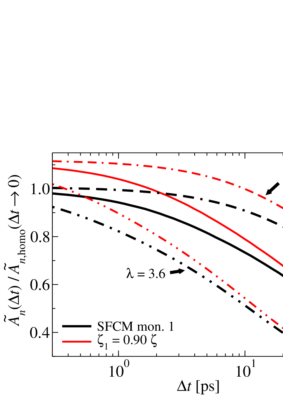
In addition, we also calculated for a SFCM, in which (a) the terminal monomers (i. e. and ) and (b) the four outermost monomers ( and ) had a different friction coefficient (or , respectively) than the other monomers (in particular , , and ). Also for the model systems with heterogeneous mobilities, the short-time value of can clearly be identified with (Fig. 2). Moreover, for a given , is nearly the same for the SFCM with at the end monomer only (scenario a) and the SFCM in which the four outermost monomers have a different -value (scenario b). Thus, also numerically, our method is able to determine on a quantitative level.
With increasing , the -curves of all models converge asymptotically towards the same long-time value, meaning also that all information about the mobility is lost. This is an important point, since it turns out that a chemically realistic polymer chain such as PEO does not display a short-time plateau because of the microscopic potentials of the backbone and its ballistic dynamics in the sub-picosecond regime (these issues are discussed in Section VI and also in our previous publications [20, 25]). Due to these effects, the for PEO can only be extracted at larger . In our previous work [20], we found that the monomer-averaged -curves for PEO and for the homogeneous SFCM agree with each other from about on, thus defining a minimum time scale for the determination of the monomeric PEO mobilities. At the same time, however, the agreement of between SFCM and PEO for also allows one to extract the PEO mobilities by comparison with the model curves. That is, the -curves in Fig 2 can be utilized to determine the relative mobility of the terminal and central PEO monomers.
The remaining issue now is to estimate in how far the -curves are still governed by the local mobility for , since the dynamics of a particular monomer will also be influenced by the other monomers in the segment beyond the microscopic time scale. Thus, it is a priori uncertain with which accuracy an unknown -value can be determined from an observed . To elucidate this, we plotted versus the underlying friction coefficient (which is known in case of the model chains) for and . It turns out that their dependence is linear (see appendix A). In particular, when normalizing both quantities by the respective values for the homogeneous SFCM, i. e. and , the data can be described by
| (15) |
which provides a translation rule between any observed and the corresponding -value. For the SFCM in which only the end monomers have a different mobility (scenario (a), see above), we find and . When the four outermost monomers have different mobilities (scenario (b)), one has larger values, i. e. and . For PEO, however, not only the mobility of the chain ends relative to the central monomers is unknown, but also how many successive monomers at the ends might be affected by the different intermolecular environment, and therefore might display a different mobility. That is, speaking in terms of the SFCM, it is unclear if scenario (a) or (b) better describes the real physical situation, and thus which model is more appropriate to determine from the PEO data. Therefore, we tested the robustness of our method by extracting according to Eq. 15 of one model using the -values of the other model. For both combinations, we find that the extracted -values deviate by no more than from the true values. Altogether, this clearly demonstrates that the local mobility of a given monomer can be determined with high precision using the SFCM curves from Fig 2.
It should be noted, however, that the dynamical behavior beyond the short-time limit also depends on the precise value of the chain stiffness (characterized by for the SFCM, see Eq. 1). However, since we already matched the characteristic ratio of the SFCM to that of PEO (section II), the interpretation of the PEO data (section VI) remains unaffected, and we refer to appendix B for a discussion of this effect.
In principle, when only comparing the model systems, one could obtain the same information from the short-time MSDs (not shown). However, for a realistic polymer chain such as PEO, the MSDs in this regime are dominated by dynamical contributions arising from the complicated, microscopic potentials (see below), whereas the model-chain behavior emerges only on longer time scales, which in turn is mainly governed by the global polymer motion. Contrarily, the analysis shown in Fig. 2 is strictly local, as is only sensitive to the relaxation of a given monomer within the local curvature . In other words, whereas all non-ideal dynamical contributions accumulate in the MSD for a realistic polymer melt, they act as random noise in the pq-analysis, provided that they are non-systematic with respect to .
In summary, the observable clearly allows the extraction of the bare mobility of a given SFCM monomer from its short-time value. Contrarily, on time scales larger than about , is also governed by the motion of the neighbor monomers, and thus rather corresponds to an effective mobility. In this regime, however, the -dependence of the SFCM curves also becomes affected by the specific value of (Eq. 1).
IV Structural Properties
Fig. 3 shows the radial distribution function of the ether oxygens of the PEO chains. This quantity has been computed for both the terminal ( and ) and the central ( and ) PEO monomers. The average has been performed over all chains in the simulation box as well as over all initial time frames. Up to approximately , two intramolecular peaks around and can be observed, corresponding to the neighbor monomer(s). The occurrence of two peaks indicates the existence of two preferred conformations (note that the root mean squared distance between the oxygen atoms of two bonded monomers is about ). Naturally, these peaks are approximately twice as high for due to chain connectivity (see inset of Fig. 3, where the curve of monomer 24 has been divided by two). When going to distances of about , one indeed observes that the terminal monomer has more intermolecular neighbors in its first coordination shell than the central monomer.

Of course, these observations are not very surprising, since the different intermolecular structure in the vicinity of terminal and central monomers seems only logical. However, as pointed out above, exactly these differences may also alter the dynamical behavior beyond the general differences due to the dissimilar chain connectivity, which are already contained in the Rouse model.
V Mean Squared Displacement
In order to get a first impression of the polymer motion, we start with the MSD, which can be regarded as the standard tool to study the dynamics in simulations. For the monomeric MSDs, one generally observes that for intermediate time scales (i. e. , with being the Rouse time) the outer monomers move faster than the central segments [4, 5, 6]. Naturally, this regime is already highly affected by the connectivity constraints of the chain, which are less present for the end monomers. This is also confirmed in Fig. 4, which shows the MSDs of the terminal and the central PEO monomers in the center-of-mass frame. As stated above, the outer monomers are faster for all shorter than , mainly as a result of the chain connectivity. The MSDs of the respective SFCM monomers are plotted as black solid (terminal) and black dashed (central) line in Fig. 4. For both the central and the outer monomers, one observes that the MSD of the SFCM is lower than the PEO curve. These deviations can be related to the more complicated local potentials for the latter system. When computing the MSD in absolute coordinates, the mismatch between PEO and SFCM becomes even worse due to the well-known, non-ideal center-of-mass motion of polymer chains in realistic melts [26, 27, 28, 18, 29], which is subtracted in Fig. 4. For these reasons, it is difficult to judge solely from the monomeric MSDs whether the Rouse assumption of a uniform also holds for the PEO melt.

VI Application of the pq-Method
Alternatively, the local dynamics of the individual PEO monomers can be evaluated by the pq-method, yielding an effective mobility free from connectivity effects. The -curves for the terminal (circles) and the central (triangles) PEO monomers as well as the corresponding curves for the SFCM with a uniform -value (black lines) are shown in Fig. 5. As above, the -axis of the model curves has been scaled by the ratio of the -values of PEO and the SFCM. The -axis has been scaled by the ratio of the mean squared Kuhn lengths and the ratio.
In case of PEO, we notice that, unlike for the SFCM, no short-time plateau emerges on time scales shorter than (not shown in Fig. 5). Rather, increases steadily with decreasing , thus yielding no direct access to the monomers’ mobilities. Of course, this behavior is not too surprising, since it seems likely that the chemical potentials and the excluded volume interactions give rise to additional systematic contributions to the short-time dynamics of PEO. However, for , one observes reasonable agreement between PEO and the SFCM for both monomer positions, demonstrating that the SFCM basically captures the local dynamical features of the PEO chains in the melt on all except shortest time scales. In particular for , for which the SFCM dynamics is still mainly governed by (see discussion in context with Fig. 2), the agreement is quantitative. This demonstrates that the short-time mobilities of the individual PEO monomers are uniformly distributed, thus confirming the classical Rouse assumption.
Apart from the short-time deviations between PEO and the SFCM, minor deviations also become noticeable for the terminal monomers on intermediate time scales, i. e. . This can also be seen in the inset of Fig. 5, which shows the curve of the terminal PEO monomer in the time window of together with the model curves from Fig. 2 (i. e. and ). It seems that the dynamics of the terminal PEO monomer on this time scale rather corresponds to that of an SFCM monomer with , although it is unclear whether this apparent agreement is just by mere coincidence. Especially due to the fact that for PEO agrees with the SFCM at , and also the central and the monomer-averaged -curves agree for all , the naive interpretation for has to be considered carefully. Within this context, it is also important to bear in mind that the dynamics on the time scale of is not solely determined by , but also by the motion of more remote monomers, and, more importantly, the details of the chemical potentials (cf. discussion of Fig. 2). Of course, in contrast to the effective-medium picture of the Rouse model or the SFCM derived thereof, the motion of the PEO monomers is not only affected by the chain connectivity, but also by intra- and intermolecular excluded volume interactions.

A first indication that these two effects (i. e. chain connectivity and correlated motion of neighbors) have a different impact on a terminal and on a central monomer is given by the following observation: The average time during which a terminal monomer diffuses a distance approximately equal to the size of its own coordination sphere (i. e. , as estimated from the extent of the first intermolecular peak in Fig. 3) is about (Fig. 4), thus falling exactly into the range of where the deviations in Fig. 5 occur. Contrarily, the average central monomer has not diffused this far until . That is, the coordination sphere of a terminal monomer itself, mostly consisting of central monomers which are intrinsically slower due to chain connectivity, relaxes on larger time scales than the self-motion of the outer monomers. In case of the central monomers, the intermolecular surroundings (modeled as frictious background in the Rouse model) relax on the same time scale as the tagged monomer.

Another fundamental difference is that a terminal monomer may exit its initial coordination sphere either by moving away from the center of the polymer chain, thus paving the way for the remaining part of the PEO molecule (subsequently termed as head monomers), or by following the contour of the rest of the chain (tail monomers, see snapshots from the MD simulations in Fig. 6, where these two events have been identified). In contrast to this, there is no such asymmetry for a monomer located in the center of the chain, as these monomers experience backdragging forces on both sides.

In order to investigate these directional correlations in more detail, we modified our analysis in the following way: For a given displacement of the terminal Kuhn segment (monomers , with center-of-mass position ), a distinction was made whether it moved in or against the direction of the -vector. In this way, one can distinguish between head monomers (), where the terminal Kuhn segment moves in front of the adjacent segments, and tail monomers (), where this segment follows the local chain contour. These two contributions to and to are shown in Fig. 7 (see also snapshots from the MD simulations in Fig. 6). For , the criterion to define head and tail monomers was if the center of mass of the subchain defined by the monomers , or, alternatively, moved in or against the direction of the bond vector of the respective Kuhn segment (see also sketch in Fig. 1). Note that in both cases the curves for the head monomers have also negative values, which result from their head-monomer definition. Naturally, trivial head and tail contributions can also be observed for the SFCM (Fig. 7) due to the bias resulting from the distinction between heads and tails. Interestingly, despite the good agreement of the average curves (in particular for ), the absolute values of both head and tail contributions for PEO are larger than for the SFCM. This is a consequence of the additional excluded volume, since for PEO all monomers within one Kuhn segment move much more correlated. Thus, the short-time displacement of a PEO monomer will already be significantly influenced by the motion of the other monomers in the segment, whereas the SFCM monomers can interpenetrate each other and thus exhibit weaker motional correlations (which even vanish in the limit ). Remarkably, for both the terminal and the central monomers, the head and tail contributions roughly cancel each other, and the local PEO dynamics in the melt is essentially the same as for a phantom chain (with minor deviations for the terminal monomers).
Of course, for PEO, one might wonder if the different coordination sphere of the terminal monomers affects the surrounding monomers themselves. For instance, it has recently been found for melts consisting of poly(propylene oxide) oligomers that the average polymer relaxation is faster compared to melts of longer chains (i. e. ), which could be attributed to the larger free volume of the chain ends[19]. In analogy, one might expect a similar effect for the local mobility. To this purpose, we calculated for all intermolecular neighbors of the terminal monomers (i. e. up to a maximum distance of , cf. Fig 3). In total, we only observe a marginal increase of of up to , which is most pronounced for time scales below and becomes negligible for larger (not shown). Thus, also the monomers in the vicinity of a chain end essentially display Rouse-like motion on local scales.
Finally, the enhanced correlations of the monomer dynamics along the PEO backbone also manifest themselves in the MSD of the center of mass of the PEO chains. Apart from the well-known subdiffusivity on time scales shorter than , which has been found in several simulations [26, 27, 28, 18, 29], experiments [28, 31] and theoretical analyses [32, 33, 29, 34, 35], we additionally observe that the center-of-mass diffusion is slightly anisotropic with respect to the orientation of the end-to-end vector . This is demonstrated by the inset of Fig. 4, which shows the ratio of the component parallel to relative to the total center-of-mass MSD, i. e. . In the absence of anisotropies one would expect an ideal ratio of . However, the actual ratio is larger for all shorter than the Rouse time ( for PEO). This shows that the preferential motion is along the primary axis of the chain, i. e. parallel to . In how far the observed anisotropy is related to the fact that real polymer coils are not spherical, but rather stretched in direction of [36, 37] might be investigated more thoroughly in future work.
In addition to these correlations, memory effects may come into play, which could cause additional differences between head and tail monomers. That is, when a monomer moves either direction, the surrounding monomers would occupy the newly available space in this scenario, and thus block the backward motion.
VII Conclusion
In this contribution, we checked the fundamental Rouse assumption of a uniform friction coefficient on all monomers for a PEO melt. The mobilities were extracted from MD simulations using our previously developed pq-method [20], which avoids the classical mode picture and rather employs a Langevin-like equation to characterize the local polymer dynamics. In contrast to the MSD, this procedure leads to the cancellation of the non-trivial terms for PEO, which arise from the additional chemical potentials. In order to interpret the local PEO dynamics, we used a semiflexible phantom chain as a reference.
During the course of our analysis it turned out that the effective mobility of both the terminal and the central PEO monomers is essentially the same as for the SFCM for . However, this agreement results from the nearly quantitative cancellation of the more complicated interactions in the PEO melt. A more detailed analysis revealed that the relaxation with respect to the local chain curvature expressed by can be decomposed in two individual contributions (head and tail monomers), depending on the direction of motion of the Kuhn segment under consideration. Due to the correlated motion in PEO arising from the excluded volume interactions, both head and tail contributions are larger for PEO. Remarkably, these contributions approximately cancel, and the mobility is roughly the same for all PEO monomers. Minor deviations (up to ten percent) only become noticeable on intermediate time scales () for the terminal monomers, for which the head and tail dynamics is not entirely equal.
As reported previously [25], our findings clearly demonstrate that the pq-method yields complementary information on the dynamics of macromolecular systems. In further work one might study in how far the chain end effects persist or enhance when approaching the glass transition temperature (cf. the Flory-Fox equation). Moreover, the pq-method is also supposed to yield fruitful results for confined polymer melts [38, 39] or complex polymer architectures [40].
Acknowledgements.
The authors would like to thank Jörg Baschnagel, Hendrik Meyer, Jean Farago and Micheal Vogel for helpful discussions and correspondence. Financial support from the NRW Graduate School of Chemistry is also greatly appreciated.Appendix A Relation between and mobility
In order to estimate in how far the -curves are governed by the local mobility for larger -values, Fig. 8 shows as a function of the underlying friction coefficient (which is known in case for the SFCM) at , , , and . By normalizing both quantities by the respective values for the homogeneous SFCM, i. e. and , the data can be described by Eq. 15. The resulting -values are presented in Table 1.

Appendix B Influence of the chain stiffness on
Fig. 9 shows for the homogeneous SFCM and for an SFCM in which the terminal monomers have a friction coefficient of for two additional values of (i. e. and , Eq. 1). One clearly observes that the different stiffness gives rise to a quantitatively different decay of , and only the asymptotic short-time limit remains unaffected. Thus, when comparing the dynamics of the SFCM with another polymer species such as PEO on larger time scales (section VI), one has to adjust the stiffness of the model chain, as e. g. done in the present work by reproducing the -value.
References
- [1] P. E. Rouse, J. Chem. Phys. 21, 1272 (1953).
- [2] M. Doi and S. F. Edwards, The Theory of Polymer Dynamics (Oxford Science Publications, Clarendon, Oxford, 2003).
- [3] P. G. de Gennes, Scaling Concepts in Polymer Physics (Cornell University Press, Ithaca, New York, 1979).
- [4] K. Kremer and G. S. Grest, J. Chem. Phys. 92, 5057 (1990).
- [5] T. Kreer, J. Baschnagel, M. Müller, and K. Binder, Macromolecules 34, 1105 (2001).
- [6] W. Paul, Chem. Phys. 284, 59 (2002).
- [7] F. Pierce, D. Perahia, and G. S. Grest, Europhys. Lett. 95, 46001 (2011).
- [8] M. Zamponi, M. Monkenbusch, L. Willner, A. Wischnewski, B. Farago, and D. Richter, Europhys. Lett. 72, 1039 (2005).
- [9] T. A. Kavassalis and J. Noolandi, Phys. Rev. Lett. 59, 2674 (1987).
- [10] T. A. Kavassalis and J. Noolandi, Macromolecules 21, 2869 (1988).
- [11] S. Rathgeber, L. Willner, D. Richter, A. Brulet, B. Farago, M. Appel, and G. Fleischer, J. Chem. Phys. 110, 10171 (1999).
- [12] T. G. Fox and P. J. Flory, J. Appl. Phys. 21, 581 (1950).
- [13] B. Schnell, H. Meyer, C. Fond, J. P. Wittmer, and J. Baschnagel, Eur. Phys. J. E 34 (2011).
- [14] T. Kitahara, S. Shimada, and H. Kashiwabara, Polymer 21, 1299 (1980).
- [15] K. A. Welp, R. P. Wool, G. Agrawal, S. K. Satija, S. Pispas, and J. Mays, Macromolecules 32, 5127 (1999).
- [16] Y. Miwa, K. Yamamoto, M. Sakaguchi, M. Sakai, S. Makita, and S. Shimada, Macromolecules 38, 832 (2005).
- [17] Y. Miwa, S. Shimada, O. Urakawa, and S. Nobukawa, Macromolecules 43, 7192 (2010).
- [18] W. Paul and G. Smith, Rep. Prog. Phys. 67, 1117 (2004).
- [19] A. Bormuth, P. Henritzi, and M. Vogel, Macromolecules 43, 8985 (2010).
- [20] D. Diddens, M. Brodeck, and A. Heuer, Europhys. Lett. 91, 66005 (2010).
- [21] R. Winkler, P. Reineker, and L. Harnau, J. Chem. Phys. 101, 8119 (1994).
- [22] A. Maitra and A. Heuer, Macromol. Chem. Phys. 208, 2215 (2007).
- [23] E. Lindahl, B. Hess, and D. van der Spoel, J. Mol. Mod. 7, 306 (2001).
- [24] O. Borodin, G. Smith, and R. Douglas, J. Phys. Chem. B 107, 6824 (2003).
- [25] D. Diddens, M. Brodeck, and A. Heuer, Europhys. Lett. 95, 56003 (2011).
- [26] W. Paul, K. Binder, D. W. Heermann, and K. Kremer, J. Chem. Phys. 95, 7726 (1991).
- [27] W. Paul, G. D. Smith, D. Y. Yoon, B. Farago, S. Rathgeber, A. Zirkel, L. Willner, and D. Richter, Phys. Rev. Lett. 80, 2346 (1998).
- [28] G. Smith, W. Paul, M. Monkenbusch, and D. Richter, Chem. Phys. 261, 61 (2000).
- [29] J. P. Wittmer, P. Polinska, H. Meyer, J. Farago, A. Johner, J. Baschnagel, and A. Cavallo, J. Chem. Phys. 134 (2011).
- [30] W. Humphrey, A. Dalke, and K. Schulten, Journal of Molecular Graphics 14, 33 (1996), http://www.ks.uiuc.edu/Research/vmd/.
- [31] M. Zamponi, A. Wischnewski, M. Monkenbusch, L. Willner, D. Richter, P. Falus, B. Farago, and M. G. Guenza, J. Phys. Chem. B 112, 16220 (2008).
- [32] K. S. Schweizer, J. Chem. Phys. 91, 5802 (1989).
- [33] M. Guenza, Phys. Rev. Lett. 88, 025901 (2001).
- [34] J. Farago, H. Meyer, and A. N. Semenov, Phys. Rev. Lett. 107 (2011).
- [35] J. Farago, H. Meyer, J. Baschnagel, and A. N. Semenov, Journal of Physics-Condensed Matter 24 (2012).
- [36] F. Eurich and P. Maass, J. Chem. Phys. 114, 7655 (2001).
- [37] C. Mischler, J. Baschnagel, and K. Binder, Adv. Colloid Interface Sci. 94, 197 (2001).
- [38] F. Varnik, J. Baschnagel, and K. Binder, Phys. Rev. E 65, 021507 (2002).
- [39] S. Peter, H. Meyer, and J. Baschnagel, J. Polym. Sci., Part B: Polym. Phys. 44, 2951 (2006).
- [40] G.-L. He, H. Merlitz, J.-U. Sommer, and C.-X. Wu, Macromolecules 40, 6721 (2007).