Constraining primordial magnetic fields through large scale structure
Abstract
We study primordial magnetic field effects on the matter perturbations in the Universe. We assume magnetic field generation prior to the big bang nucleosynthesis (BBN), i.e. during the radiation dominated epoch of the Universe expansion, but do not limit analysis by considering a particular magnetogenesis scenario. Contrary to previous studies, we limit the total magnetic field energy density and not the smoothed amplitude of the magnetic field at large (order of 1 Mpc) scales. We review several cosmological signatures, such as halos abundance, thermal Sunyaev Zel’dovich (tSZ) effect, and Lyman- data. For a cross check we compare our limits with that obtained through the CMB faraday rotation effect and BBN. The limits are ranging between 1.5 nG and 4.5 nG for .
Subject headings
primordial magnetic fields; early universe; large scale structureI. Introduction
Observations show that galaxies have magnetic fields with a component that is coherent over a large fraction of the galaxy with field strength of order Gauss (G) [8, 71, 65]. These fields are supposed to be the result of amplification of initial weak seed fields of unknown nature. A recent study, based on the correlation of Faraday rotation measures and MgII absorption lines (which trace halos of galaxies), indicates that coherent G-strength magnetic fields were already in place in normal galaxies (like the Milky Way) when the universe was less than half its present age [43]. This places strong constraints both on the strength of the initial magnetic seed field and the time-scale required for amplification. Understanding the origin and evolution of these fields is one of the challenging questions of modern astrophysics. There are two generation scenarios under discussion currently: a bottom-up (astrophysical) one, where the needed seed field is generated on smaller scales; and, a top-down (cosmological) scenario, where the seed field is generated prior to galaxy formation in the early universe on scales that are large now. More precisely, astrophysical seed field sources include battery mechanisms, plasma processes, or simple transport of magnetic flux from compact systems (e.g. stars, AGNs), where magnetic field generation can be extremely fast because of the rapid rotation [44]. Obviously, the correlation length of such a seed field cannot be larger than a characteristic galactic length scale, and is typically much smaller. In the cosmological seed field scenario, [35], the seed field correlation length could be significantly larger than the current Hubble radius, if it was generated by quantum fluctuations during inflation. There are different options for seed field amplification, ranging from the MHD dynamo to the adiabatic compression of the magnetic field lines during structure formation [8]. The presence of turbulence in cosmic plasma plays a crucial role in both of these processes. The MHD turbulence was investigated a long time ago when considering the processes in astrophysical plasma, while there is a lack of studies when addressing the turbulence effects in cosmological contexts [10]. In the late stages of evolution the energy density present in the form of turbulent motions in clusters can be as large as 5-10% of the thermal energy density [42]. This can influence the physics of clusters [60], and/or at least should be modeled correctly when performing large scale simulations [66, 25]. The proper accounting of the MHD turbulence effects is still under discussion [58]. Both astrophysical and primordial turbulence might have distinctive observational signatures. As we already noted above, the most direct signature of MHD turbulence is the observed magnetic fields in clusters and galaxies.
Galactic magnetic fields are usually measured through the induced Faraday rotation effect (see [65]) and, as mentioned above, the coherent field magnitude is of order a few G with a typical coherence scale of 10 kpc.11 1 On the other hand, simulations starting from constant comoving magnetic fields of G show clusters generating fields sufficiently large to explain Faraday rotation measurements [19, 5]. On larger scales there have been recent claims of an observed lower limit of order G on the intergalactic magnetic field [49, 63, 20], assuming a correlation length of Mpc, or possibly two orders of magnitude smaller [18]. An alternative approach to explain the blazar spectra anomalies has been discussed by [13], where two beam plasma instabilities were considered.22 2 The recent study [2] claims that proper accounting for uncertainties of the source modeling leads to consistence with a zero magnetic field hypothesis. Although these instabilities are well tested through numerical experiments for laboratory plasma for a given set of parameters such as a temperature and energy densities of beams and background, its efficiency might be questioned for cosmological plasma because of a significantly different (several orders of magnitudes) beam, and background temperature and energy densities. Prior to these observations, the intergalactic magnetic field was limited only to be smaller than a few nG from cosmological observations, such as the limits on the cosmic microwave background (CMB) radiation polarization plane rotation [67] and on the Faraday rotation of polarized emission from distant blazars and quasars [11].
In the present paper we consider the presence of a primordial magnetic field in the Universe and give a simplified description of its effect on large scale structure formation. We assume that the magnetic field has been generated during the radiation dominated epoch and prior to big bang nucleosynthesis (BBN). Since the magnetic energy density contributes to the relativistic component, the presence of such a magnetic field affects the moment of matter-radiation equality, shifting it to a later stages. We focus on the linear matter power spectrum in order to show that even if the total energy density present in the magnetic field (and as a consequence in magnetized turbulence) is small enough, its effects might be substantial, and the effect becomes stronger due to non-linearity of processes under consideration.
It has become conventional to derive the cosmological effects of a seed magnetic field by using its spectral shape (parameterized by the spectral index ) and the smoothed value of the magnetic field () at a given scale (which is usually taken to be 1 Mpc). In [34] we developed a different and more adequate formalism based on the effective magnetic field value that is determined by the total energy density of the magnetic field. Such an approach has been mostly motivated by the simplest energy constraint on the magnetic field generated in the early universe. In order to preserve BBN physics, only 10% of the relativistic energy density can be added to the radiation energy density, leading to the limit on the total magnetic field energy density corresponding to the effective magnetic field value order of G. More precise studies of the influence of the primordial magnetic field on the expansion rate and the abundance of light elements performed recently [68, 36], lead to effective magnetic field amplitudes with order of G.
The described formalism has been applied to describe two different effects of the primordial magnetic field; the CMB Faraday rotation effect and mass dispersion [33]. As a striking consequence, we show that even an extremely small smoothed magnetic field of G at 1 Mpc, with the Batchelor spectral shape () at large scales, can leave detectable signatures in CMB or LSS statistics. In the present investigation we focus on the thermal Sunyaev-Zel’dovich effect, the cluster number density, and Lyman- data. The large scale based tests such as tSZ, Lyman-, cosmic shear (gravitational lensing), X-rays cluster surveys, have been studied in [56, 61, 62, 24, 50], but again in the context of a smoothed magnetic field. Another possible observational signature of large-scale correlated cosmological magnetic fields may be found in cosmic ray acceleration, and corresponding gamma ray signals, (see Ref. [23] and references therein). These observational signatures of the primordial magnetic field are beyond the scope of the present paper. We also do a more precise data analysis, and we do not focus only on inflation-generated magnetic fields.
The structure of the paper is as follows. In Sec. II we briefly review the effective magnetic field formalism and discuss the effect on the density perturbations. In Sec. III we review observational consequences and derive the limits on primordial magnetic fields. Conclusions are given in Sec. IV.
II. Modeling the Magnetic Field Induced Matter Power Spectrum
We assume that the primordial magnetic field has been generated during or prior to BBN, i.e., well during the radiation dominated epoch.33 3 Note that some results of this paper can be applied also to the case when magnetic fields are generated during the matter dominated epoch, but with several ”caveats”: in this case the BBN limits will not be valid, since the magnetic field will not be present during matter-radiation equality and will not affect the expansion rate of the early universe and light element abundances. On the other hand, if the magnetic field has been generated prior to recombination, the CMB limits must be used. For any other field generated before reionization and first structure formation only the large-scale structure tests may apply. We thank the anonymous referee for pointing out this issue. A stochastic Gaussian magnetic field is fully described by its two-point correlation function. For simplicity, we consider the case of a non-helical magnetic field44 4 We limit ourselves to considering a non-helical magnetic field because the density perturbations, and as a result the matter power spectrum, is not affected by the presence of magnetic helicity., for which the two-point correlation function in wavenumber space is [33]
| (1) |
Here, and are spatial indices; , is a unit wavevector; is the transverse plane projector; is the Dirac delta function, and is the power spectrum of the magnetic field.
The smoothed magnetic field is defined through the mean-square magnetic field, , where the smoothing is done on a comoving length with a Gaussian smoothing kernel function . Corresponding to the smoothing length is the smoothing wavenumber . The power spectrum is assumed to depend on as a simple power law function on large scales, (where is the cutoff wavenumber),
| (2) |
and assumed to vanish on small scales where .
We define the effective magnetic field through the magnetic energy density . In terms of the smoothed field, the magnetic energy density is given by
| (3) |
and thus . For the scale-invariant spectrum and for all values of . The scale-invariant spectrum is the only case where the values of the effective and smoothed fields coincide. For causal magnetic fields with the smoothed magnetic field value is extremely small for moderate values of the magnetic field.
We also need to determine the cut-off scale . We assume that the cut-off scale is determined by the Alfvén wave damping scale , where is the Alfvén velocity and is the Silk damping scale [31, 59]. Such a description is more appropriate when dealing with a homogeneous magnetic field, and the Alfvén waves are the fluctuations of with respect to a background homogeneous magnetic field (). In the case of a stochastic magnetic field we generalize the Alfvén velocity definition from [47], by referring to the analogy between the effective magnetic field and the homogeneous magnetic field. Assuming that the Alfvén velocity is determined by , a simple computation gives the expression of in terms of :
| (4) |
Here is the Hubble constant in units of 100 km s-1 Mpc-1.
Note that any primordial magnetic field generated prior or during BBN should satisfy the BBN bound (for a recent studies of primordial magnetic fields effects on BBN processes and corresponding limits see [68, 36]). Assuming that the magnetic field energy density is not damped away by MHD processes, the BBN limit on the effective magnetic field strength, G, while transferred in terms of the BBN bounds results in extremely small values for causal fields, see [15, 34].
The primordial magnetic field affects all three kinds of metric perturbations, scalar (density), vector (vorticity), and tensor (gravitational waves) modes through the Einstein equations. The primordial magnetic field generates a matter perturbation power spectrum with a different shape compared to the standard CDM model. As we noted above in this paper we focus on matter perturbations. As it has been shown by [37, 26], the magnetic-field-induced matter power spectrum for and for .

This in turn affects the formation of rare objects like galaxy clusters which sample the exponential tail of the mass function. [56] study in great detail the formation of the magnetic field matter power spectrum through analytical description, and provide a modified version of CAMB that includes the possibility of a non-zero magnetic field. We have used the CAMB code to determine the matter power spectra for a wide range of the magnetic field amplitudes and spectral indices. These spectra are shown in Fig. (1). It is obvious that the matter power spectrum is sensitive to the values of the cosmological parameters: the Hubble constant in units of 100 kmMpc, , , and , as well as the density parameter of each dark matter component, i.e., and (here, , , , and indices refer to matter, baryons, cold dark matter, and neutrinos respectively, and is the density parameter. To generate the matter plot we assume the standard flat CDM model with zero curvature, and we use the following cosmological parameters: , , and . For simplicity, we assume massless neutrinos with three generations.55 5 The standard CDM model matter power spectrum assumes a close to scale-invariant (Harrison-Peebles-Yu-Zel’dovich) post-inflation energy density perturbation power spectrum , with . As we can see the increase of the smoothed field amplitude results in the additional power spectrum shift to the left, while increasing the value of makes the vertical shift. As we can see the large-scale tail (small wavenumbers) of the matter power spectrum is unaffected by the presence of the magnetic field. Below we address some of effects induced by the presence of the magnetic field, especially on large scales.
III. Observational Signatures
Primordial magnetic fields can play a potentially important role in the formation of the first large-scale structures.
III.1. The Thermal Sunyaev-Zel’dovich effect
As demonstrated in [56, 61, 51] the strength of the primordial magnetic field affects the growth of structure. The power spectrum of secondary anisotropies in the CMB caused by the thermal Sunyaev-Zel’dovich effect (tSZ) is a highly sensitive probe of the growth of structure [39, e.g.]. The tSZ angular power spectrum probes the distribution of galaxy clusters on the sky essentially out to any redshift. At , half of the contribution to the SZ power spectrum comes from matter halos with masses greater than at redshifts less than , see [7, 64].

All the previous work on how primordial magnetic fields affect the tSZ power spectrum have used the model from [39], here referred to as KS model, which has been shown to be incompatible with recent observations of clusters [3] and tSZ power spectrum measurements by [46]. Using the KS model for primordial magnetic field studies also ignores all the recent advancements in tSZ power spectrum theory and predictions that illustrate the importance of properly modeling the detailed astrophysics of the intracluster medium [6, 7, 55, 64, e.g.]. We modify the code described in [56] to include these improvements by changing the pressure profile used in their model from KS to the profile given in [6, 7]. The results from the new pressure profile are shown in Fig. (2) with the greatest difference being the amplitude of the new tSZ power spectrum is approximately two times lower than previous predictions and below the current observational constraint from ACT [21] and SPT [53] at . Updating the theory predictions for the tSZ power significantly reduces the constraints put on primordial magnetic field parameters using these observations. In Fig. (2) we illustrate that magnetic fields with an effective amplitude of order of 5 nG are almost excluded. Given that there is additional uncertainty in the theoretical modeling of the tSZ [6, 7, 55, 64, e.g.], combined with significant contributions from other secondary sources [53, 21] around , for example from dusty star forming galaxies, future tSZ power spectrum measurements are not going to be competitive in constraining primordial magnetic fields parameters.
III.2. Halo Number Density
The predicted halo number density depends on the considered cosmological model. One of important characteristics of a cosmological model is the linear matter power spectrum that we reviewed in Sec. II above. Below we discuss the halo number count dependence on the presence of the magnetic field.
The halo mass function at a redshift is , where is the comoving number density of collapsed objects with mass lying in the interval , and it can be expressed as
| (5) |
The multiplicity function is a universal function of the peak height [52] , where is the r.m.s. amplitude of density fluctuations smoothed over a sphere of radius , and the critical density contrast is the density contrast for a linear overdensity able to collapse at the redshift . Here, is the mean matter density at the redshift . For gaussian fluctuations [52], where the normalization constant is fixed by the requirement that all of the mass lie in a given halo [70]. The evolution of the halo mass function is mostly determined by the dependence of .
The r.m.s amplitude of density fluctuations is related to the linear matter power spectrum through [32]
| (6) |
where is the growth factor of linear perturbations normalized as today, is the Fourier transform of the top-hat window function, . In Fig. 3 we illustrate the function for the different values of the effective magnetic field, , and the spectral index . The smaller amplitude of the magnetic field results in modifications at smaller mass scales. The dependence on the magnetic field characteristics is also derived in [33], but contrary to the case presented here, reflects only the induced by the pure magnetic field. In the present work we derive the effect from the magnetic field on the overall matter dispersion, including the standard density perturbations. The value of at is around 0.8 agreeing well with observational data, see [14].
Numerical computation results for are not accurately fit by the PS expression , see Refs. [57, 32, 30]. Several more accurate modifications of have been proposed. Here, we use the ST modification [57], as defined, (see Eq. 5 of Ref. [70])
| (7) |
where the parameters , and are fixed by fitting to the numerical results [69] (for the PS case: and ) [57]. With this choice of parameter values the mass of collapsed objects in Eq. (7) must be defined using a fixed over-density contrast with respect to the background density , and this requires accounting for the mass conversion between and . Such a conversion depends on cosmological parameters, (see Fig. 1 of [69]). Here, we use an analytical extrapolation of this figure to do the conversion for .
The difference induced by the magnetic field in the matter power spectrum can potentially modify the parameter entering in Eq. (7), that will result in different halo number counts. On the other hand, here we focus on the first order effects, so we neglect all changes induced by the magnetic field in the Sheth-Tolmen model parameter fitting (see [57]). We also use the halo number count function at because we are focusing only on the linear power spectrum, and all effects related to the magnetic field non-linear evolution (see [54]) during the structure formation are neglected. We will present a more realistic scenario of the first object formation in future works.


In Fig. (4) (top panel) we illustrate the halo mass function today () for different values of and . As we can see, the magnetic field presence affects the small mass ranges, reducing the abundance of low mass objects. We do not present here any statistics using halo data accounting for several uncertainties involving clusters physics [7]. On the other hand, we would like to underline that the presence of a high enough magnetic field might be a possible explanation of the low mass objects abundance, which is one of the unsolved puzzles in CDM cosmologies.
To get a better understanding of the magnetic field influence on the halo abundance, we plot the ratio of halo number density of CDM models with and without magnetic fields (see Fig. 4, bottom panel). In the high mass limit all magnetized CDM models compared to the CDM model predict slightly (a relative difference of the order of ) higher halo number density. Number density excess peaks around halos with mass () and is strongly affected by the effective magnetic field value, as well as on the spectral shape. In contrast, at low mass limit , number of objects can be significantly lower as then its non-magnetic value.
III.3. Lyman- data
The small scale modifications induced by the primordial magnetic field must be reflected in first object formation in the Universe, i.e., the objects at high redshifts. The most important class of such objects are damped Lyman- absorption systems.66 6 These objects have a high column density of neutral hydrogen (cm-2) and are detected by means of absorption lines in quasar spectra [72]. Observations at high redshift have lead to estimates of the abundance of neutral hydrogen in damped Lyman- systems [45]. The standard view is that damped Lyman- systems are a population of protogalactic disks [72], with a minimum mass of [28]. To describe these systems it is possible to use semi-analytical modeling. Lyman- systems has been used to constrain different cosmological scenarios, see Ref. [48], and references therein. Lyman- data is very sensitive to the matter power spectrum around Mpc-1, wavenumbers that are affected by the primordial magnetic field [56]. As we will see below these systems can be used to place stringent constraints on magnetic field properties.
We do not go through the detailed modeling of Lyman- systems, leaving this for more precise computations, but we use the direct comparison of the reconstructed matter power spectrum and the theoretical matter power spectra affected by the primordial magnetic field.
For this study we use Lyman- data obtained by the Keck telescope [17]. To get a conversion of data points (accounting that we use the wavevector units Mpc, we multiply data by the conversion factor
given in Ref. [37]. As the data is given at redshift 2.72, we translate the data to redshift zero by multiplying it by the square of the ratio of the growth factor at redshift zero to that at redshift 2.72. We compute the growth factors using the ICOSMOS calculator.77 7 ICOSMOS Calculator is available at http://www.icosmos.co.uk/index.html. Thus, we multiply the data by 8.145 to estimate the Lyman-α data at redshift z = 0. The comparison of the theoretical predicted matter power spectrum and Lyman- data is given in Fig. (5).

We use statistics to compare the predicted model with Lyman- data. We assume no correlation between the uncertainties in the measurements for different values and find no evidence for primordial magnetic fields.
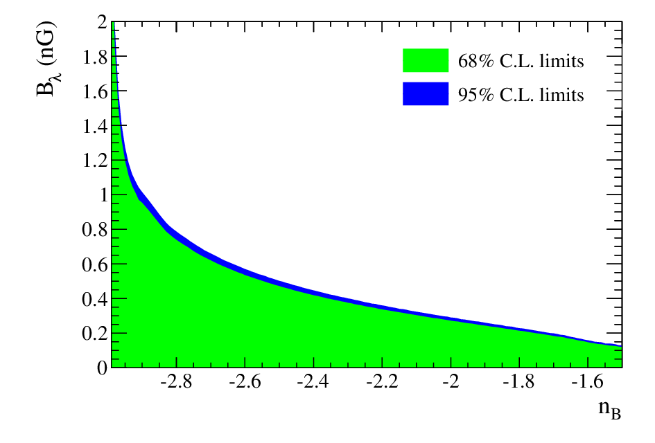
The 95% and 68% confidence level limits are given in Fig. 6. The limits on are given Fig. 7. We explicitly present the limits for and just to show that they have different behaviors when the spectral index is increasing. In terms of the total energy density of the magnetic field the limits are weaker if we are considering the redder spectra. At this point the total energy density of the phase transition generated magnetic field is almost unconstrained.

III.4. The CMB Faraday Rotation effect
As we have already noted above the primordial magnetic field induces CMB polarization Faraday rotation, and for a homogeneous magnetic field the rotation angle is given by, [41]
| (8) |
where is the amplitude of the magnetic field, and is the frequency of the CMB photons. In the case of a stochastic magnetic field we have to determine the r.m.s. value of the rotation angle, , and the corresponding expression in terms of the effective magnetic field is given in [33], being
| (9) | |||||
Here, is the present value of conformal time, is a Bessel function with argument , and where is the Silk damping scale. In the case of an extreme magnetic field which just satisfies the BBN bound, might become less than the Silk damping scale. In this case the upper limit in the integral above must be replaced by . Note, that for , Eq. (9) is reduced to Eq. (8) (see for details Ref. [33].
Here, we quote Ref. [40] in order to determine the upper limits for the r.m.s. rotation angle. Adding the statistical and systematic errors in quadrature and averaging over WMAP [40], QUaD [1] and BICEP [16] (see for more details Ref. [40]) with inverse variance weighting, the limits obtained were at (68% CL), or (95% CL). We obtain for the r.m.s. value (absolute) of the rotation angle and (68% C.L. and 95% C.L., respectively) assuming gaussian statistics. In Fig. (8) we display the upper limits of the effective magnetic field using the rotation angle constraints quoted above. Note that these limits are an order of magnitude better than obtained previously in Ref. [33] where we used the WMAP 7 year data alone. For almost scale-invariant magnetic field the limits are around 0.5 nG. As we can see for the BBN limits on the effective magnetic field strength are stronger than those coming from the CMB faraday rotation effect. The situation is completely different when determining the limits for the smoothed magnetic field with , which are extremely strong from BBN [15, 34], and moderate in the case of the large scale structures or the CMB birefrigence, see above.

IV. Conclusion
In this paper we studied the large-scale signatures of cosmological magnetic fields generated during the radiation dominated epoch prior to the BBN. We address such effects as the thermal Sunyaev-Zel’dovich effect, halo number density, and Lyman- data. Due to several uncertainties present in tSZ and halo abundance tests we find that Lyman- measurements provide the tightest constraints on the primordial magnetic field energy density. We express these limits in terms of the effective value of the magnetic field, . In the case of the scale invariant spectrum these limits are identical to limits on the smoothed magnetic field , (smoothed over a length scale that is conventionally taken to be 1 Mpc). For a steep magnetic field with spectral index the difference between the limits derived in terms of the effective and smoothed field is several orders of magnitude. Also limits have different behavior with increasing . At this point, as we underlined previously [33] using the smoothed magnetic field can result in some confusion: the smoothed magnetic field at 1 Mpc scales is extremely small, while the total energy density of the magnetic field is maximal allowed by BBN bounds (see Refs. [68, 36] for more details on BBN bounds). The small values of the magnetic fields for (that corresponds to the phase transition generated magnetic fields) might be treated as non-relevance on these fields. For example, in Ref. [56] it is claimed that the magnetic field with the spectral index greater than -2.5 is excluded [56], while as it is shown in Ref. [34] the magnetic field with extremely small smoothed field value at Mpc order of Gauss with the spectral index can leave observable traces on the CMB and large scale structure formation. The limits range between 1.5 nG and 4.5 nG for . These limits are comparable for those from the CMB polarization plane rotation. Our results can be applied with some precautions to the primordial magnetic fields generated in the matter dominated epoch too, see sec. 2.
Note when this paper was in final stage of preparation Ref. [50] appeared showing that magnetic fields can be strongly constrained by first object formation, in particular through Lyman- data.
We acknowledge useful comments from the anonymous referee. We are greatly thankful to R. Shaw for useful comments and discussion. The computation of the magnetic field power spectrum has been performed using the modified version of CAMB, for details see [56]. We appreciate useful discussions with A. Brandenburg, L. Campanelli, R. Croft, R. Durrer, A. Kosowsky, A. Kravtsov, F. Miniati, K. Pandey, B. Ratra, U. Seljak, S. Sethi, and R. Sheth. We acknowledge partial support from Swiss National Science Foundation SCOPES grant 128040, NSF grants AST-1109180, NASA Astrophysics Theory Program grant NNXlOAC85G. T.K. acknowledges the ICTP associate membership program. A.N and N.B. are supported by a McWilliams Center for Cosmology Postdoctoral Fellowship made possible by Bruce and Astrid McWilliams Center for Cosmology. A.T. acknowledges the hospitality of the McWilliams Center for Cosmology.
References
- [1] Ade, P. et al. [QUaD Collaboration], 2008, Astrophys. J. 674, 22.
- [2] Arlen, T. C., Vassiliev, V. V., Weisgarber, T., Wakely, S. P., and Shafi, S. V., arXiv:1210.2802 [astro-ph.HE].
- [3] Arnaud, M, Pratt, G. W., Piffaretti, R., Boehringer, H., J. H. Croston, J. H., and Pointecouteau, E., 2010, Astron. and Astrophys., 517, A92.
- [4] Banerjee, R., and Jedamzik, K. 2004, Phys. Rev. D, 70, 123003.
- [5] Banerjee, R., and Jedamzik, K. 2003, Phys. Rev. Lett., 91, 251301.
- [6] Battaglia, N., Bond, J. R., Pfrommer, C., Sievers, J. L., and Sijacki, D., 2010, Astrophys. J. 725, 91.
- [7] Battaglia, N., Bond, J. R., Pfrommer, C., and Sievers, J. L., 2012, Astrophys. J. 758, 75.
- [8] Beck, R., Brandenburg, A., Moss, D., Shukurov, A., & Sokoloff, D. 1996, ARA&A, 34, 155
- [9] Bernet, M. L., Miniati, F., Lilly, S. J., Kronberg, P. P., and Dessauges-Zavadsky, M., 2008, Nature 454, 302.
- [10] Biskamp, D. 2003, Magnetohydrodynamic Turbulence (Cambridge University, Cambridge);
- [11] Blasi, P., S. Burles, S., Olinto, A. V., 1999, Astrophys. J. 514, L79.
- [12] Brandenburg, A., Enqvist, K., and Olesen, P. 1996, Phys. Rev. D, 54, 1291.
- [13] Broderick, A. E., Chang, P., and Pfrommer, C., 2012, Astrophys. J. 752, 22.
- [14] Burenin, R. A. and Vikhlinin, A. A., 2012, Astron. Lett. 38, 347.
- [15] Caprini, C., and Durrer, R., 2001, Phys. Rev. D. 65 023517.
- [16] Chiang, H. C., Ade, P. A. R., Barkats, D., Battle, J. G., et al., 2010, Astrophys. J. 711, 1123.
- [17] Croft, R. A. C., et al., (2002) Astron. Astrophys. 581, 20.
- [18] Dermer, C. D., Cavaldini, M., Razzaque, S., Finke, J.D., Chiang, J., Lott, B., 2011 ApJ733, L21.
- [19] Dolag, K., Bartelmann, M., and Lesch, H. 2002, A&A, 387, 383
- [20] Dolag, K., Kachelriess, M., Ostapchenko, S. and Tomas, R., 2011, ApJ727, L4.
- [21] Dunkley, J., Hlozek, R., Sievers, J., Acquaviva, V., Ade, P. A. R. Aguirre, P., Amiri, M., and Appel, J. W., et al., 2011, Astrophys. J. 739, 52.
- [22] Durrer, R. and Caprini, C. 2003, J. Cosmology Astropart. Phys., 0311, 010.
- [23] Essey, W., Ando, A. A., and Kusenko, A., 2012, Astropart. Phys. 35, 135.
- [24] Fedeli, C. and L. Moscardini, L., arXiv:1209.6332 [astro-ph.CO].
- [25] Fang, T., Humphrey, P. J., and Buote, D. A., 2009, Astrophys. J. 691, 1648.
- [26] Gopal, R. and Sethi, S. K., 2005 Phys. Rev. D 72, 103003.
- [27] Grasso D. and H.R. Rubinstein, H. R., 2001, Phys. Rev. D348, 163.
- [28] Haehnelt, M.G., 1995, Mon. Not. Roy. Astron. Soc. 273 , 249.
- [29] Hogan, C. J. 1983, Phys. Rev. Lett., 51, 1488.
- [30] Hu, W. and Kravtsov, A., 2003, Astrophys. J. 584, 702.
- [31] Jedamzik, K., Katalinic, V., and Olinto, A. V, 1998 Phys. Rev. D 57, 3264.
- [32] Jenkins, A. and Frenk, C. S. and White, S. D. M. and Colberg, J. M. and Cole, S. and Evrard, A. E. and Couchman, H. M. P. and Yoshida, N., 2001, Mon. Not. Roy. Astron. Soc. ]bf 321 372.
- [33] Kahniashvili, T., Tevzadze, A. G., Sethi, S., Pandey, K., and Ratra, B., 2010, Phys. Rev. D 82, 083005.
- [34] Kahniashvili, T., Tevzadze, A. G., and Ratra, B., 2011, ApJ, 726, 78.
- [35] Kandus, A., Kunze, K. E., and Tsagas, C. G., 2011, Phys. Rept. 505, 1.
- [36] Kawasaki, M. and Kusakabe, M., 2012 Phys. Rev. D 86, 063003
- [37] Kim, E., Olinto, A. V., and Rosner, R., 1996, Astrophys. J. 468, 28.
- [38] Kim, T. S., et al., 2004, Mon. Not. Roy. Astron. Soc. 347, 355.
- [39] Komatsu, E. and Seljak, U., 2002, cosmological parameters,” Mon. Not. Roy. Astron. Soc. 336, 1256.
- [40] Komatsu, E., et al. [WMAP Collaboration] 2011, Astrophys. J. Suppl. 192, 18.
- [41] Kosowsky, A. and Loeb, A., 1996, Astrophys. J. 469, 1.
- [42] Kravtsov, A. and Borgani, S. 2012, Annual Rev. of Astron. and Astrophys., 50, 353.
- [43] Kronberg, P. P., M. L. Bernet, M. L., Miniati, F., Lilly, S. J., Short, M. B., and Higdon, D. N., 2008, Astrophys. J, 676, 70.
- [44] Kulsrud, R. M. and Zweibel, E. G., 2008, Rept. Prog. Phys. 71, 0046091.
- [45] Lanzetta, K.M., Wolfe, A.M. and Turnshek, D.A. 1995, Astrophys. J 440, 435.
- [46] Lueker, M., Reichardt, C. L., Schaffer, K. K., Zahn, O., Ade, P. A. R., Aird, K.A., Benson, B. A., and Bleem L. E., et al., 2010, Anisotropies with the South Pole Telescope,” Astrophys. J. 719, 1045.
- [47] Mack, A., Kahniashvili, T., and Kosowsky, A., 2002, Phys. Rev. D 65, 123004.
- [48] McDonald, P, Seljak, U., Cen, R., Shih, D., Weinberg, D. H., Burles, S., Schneider, D. P., Schlegel, D. J., Bahcall, N. A., Briggs, S. W. et al., 2005, Astrophys. J. 635, 761,
- [49] Neronov, A., and Vovk, I., 2010, Science 328, 73.
- [50] Pandey K. L. and Sethi, S. K., 2012 arXiv:1210.3298 [astro-ph.CO].
- [51] Paoletti, D. and Finelli, F., 2012 Fields with WMAP and South Pole Telescope data,” arXiv:1208.2625 [astro-ph.CO].
- [52] Press, W. H., and Schechter, P., 1974, Astrophys. J. 187, 425.
- [53] Reichardt, C. L., Shaw, L., Zahn, O., , Aird, K. A., Benson, S. A., Bleem, L. E., J. E. Carlstrom, J. E., and C. L. Chang C. L., et al., 2012, anisotropies with two years of South Pole Telescope observations,” Astrophys. J. 755, 70.
- [54] D. R. G. Schleicher and F. Miniati, 2011, Mon. Roy. Not Ast. Soc. 418 L143.
- [55] Shaw, L. D. Nagai, D., Bhattacharya, S., and Lau, E. T., 2010, Astrophys. J. 725, 1452.
- [56] Shaw, J. R. and A. Lewis, A., 2012, Phys. Rev. D 86, 043510.
- [57] Sheth, R. K. and Tormen, G., 1999, Mon. Not. Roy. Astron. Soc. 308, 119.
- [58] Springel, V., 2010, Ann. Rev. Astron. Astrophys. 48, 391.
- [59] Subramanian, K. and Barrow, J. D., 1998, Phys. Rev. D 58, 083502.
- [60] Subramanian, K., Shukurov, A., and Haugen, N. E. L. 2006, Mon. Not. Roy. Astron. Soc. 366, 1437.
- [61] Tashiro, H. and Sugiyama, N., 2011, Mon. Not. Roy. Astron. Soc. 411, 1284.
- [62] Tashiro, H., Takahashi, K., and Ichiki, K., 2012, Mon. Not. Roy. Astron. Soc. 424, 927.
- [63] Tavecchio, F., Ghisellini, G., Foschini, L., Bonnoli, G., Ghirlanda, G., and Coppi,P., 2010, Mon. Not. Roy. Astron. Soc. 406, L70.
- [64] Trac, H., Bode, P., and Ostriker, J. P., 2011, Astrophys. J. 727, 94.
- [65] Vallée, J. P. 2004, New Astron. Rev., 48, 763.
- [66] Vazza, F., Tormen, G., Cassano, F., Brunetti, G., and Dolag, K., 2006, Mon. Not. Roy. Astron. Soc. Lett. 369, L14.
- [67] Yamazaki, D. G., Ichiki, K,, Kajino, T., and Mathews, G. J., 2012, Adv. Astron. 2010, 586590.
- [68] Yamazaki, D. G. and M. Kusakabe, M., 2012 Phys. Rev. D. 86, 123006.
- [69] White, M., 2001, Astron. Astrophys. 367, 27.
- [70] White, M. 2002, Astrophys. J. Supl. 143, 241.
- [71] Widrow, L. M. 2002, Rev. Mod. Phys., 74, 775.
- [72] Wolfe, A., 1993, in Relativistic Astrophysics and Particle Cosmology , eds. C.W., Ackerlof, M.A., Srednicki ( New York: New York Academy of Science ) , p.281