跳到论文正文
W Papers独立论文阅读器 arXiv:1211.2763 论文正文 计算阅读时间 · 0%
引用这篇论文根据当前论文元数据生成,正式投稿前建议核对。


License: arXiv.org perpetual non-exclusive license
arXiv:1211.2763v2 [math.ST] 09 Jan 2014

Global smoothness estimation of a Gaussian process from regular sequence designs

Delphine Blanke Address: Avignon Université, LMA EA2151, 33 rue Louis Pasteur, F-84000 Avignon, France. Email address: delphine.blanke@univ-avignon.fr and Céline Vial Address: Université de Lyon, CNRS UMR 5208, Polytech Lyon-Université de Lyon 1, Institut Camille Jordan, 43 blvd du 11 novembre 1918, 69622 Villeurbanne Cedex, France. Email address: celine.vial@univ-lyon1.fr
Abstract.

We consider a real Gaussian process XX having a global unknown smoothness (r0,β0CLOSE(r_{\scriptscriptstyle 0},\beta_{\scriptscriptstyle 0}), r0∈ℕ0r_{\scriptscriptstyle 0}\in{\mathds{N}}_{0} and β0∈]0,1[\beta_{\scriptscriptstyle 0}\in]0,1[, with X(r0)X^{(r_{\scriptscriptstyle 0})} (the mean-square derivative of XX if r0≥1r_{\scriptscriptstyle 0}\geq 1) supposed to be locally stationary with index β0\beta_{\scriptscriptstyle 0}. From the behavior of quadratic variations built on divided differences of XX, we derive an estimator of (r0,β0)(r_{\scriptscriptstyle 0},\beta_{\scriptscriptstyle 0}) based on - not necessarily equally spaced - observations of XX. Various numerical studies of these estimators exhibit their properties for finite sample size and different types of processes, and are also completed by two examples of application to real data.

Key words and phrases:
Inference for Gaussian processes; Locally stationary process; Divided differences; Quadratic variations

1. Introduction

In many areas assessing the regularity of a Gaussian process represents still and always an important issue. In a straightforward way, it allows to give accurate estimates for approximation or integration of sampled process. An important example is the kriging, which becomes more and more popular with growing number of applications. This method consists in interpolating a Gaussian random field observed only in few points. Estimating the covariance function is often the first step before plug this estimates in the Kriging equations, see Stein (1999). Usually the covariance function is assumed to belong to a parametric family, where these unknown parameters are linked to the sampled path regularity: for example the power model, which corresponds to a Fractional Brownian motion. Actually, many applications make use of irregular sampling and Stein (1999) (chap. 6.9) gives an hint of how adding three points very near from the origin among the already twenty equally spaced observations improve drastically the estimation of the regularity parameter. In this paper, we defined an estimator of global regularity of a Gaussian process when the sampling design is regular, that is observation points correspond to quantile of some distribution, see section 2 for details. Taking into account a non uniform design is innovating regarding other existing estimators and makes sense as to the remark above.

A wide range of methods have been proposed to reconstruct a sample path from discrete observations. For processes satisfying to the so-called Sacks and Ylvisaker (SY) conditions, recent works include: Müller-Gronbach (1996, orthogonal projection, optimal designs), Müller-Gronbach and Ritter (1997, linear interpolation, optimal designs), Müller-Gronbach and Ritter (1998, linear interpolation, adaptive designs). Under Hölder type conditions, one may cite e.g. works of Seleznjev (1996, linear interpolation), Seleznjev (2000, Hermite interpolation splines, optimal designs), Seleznjev and Buslaev (1998, best approximation order). Note that a more detailed survey may be found in the book by Ritter (2000). Another important topic, involving the knowledge of regularity and arising in above cited works, is the search of an optimal design. In time series context, Cambanis (1985) analyzes three important problems (estimation of regression coefficients, estimation of random integrals and detection of signal in noise) for which he is looking for optimal design. The latter two problems involve approximations of integrals, where knowledge of process regularity is particularly important (Ritter, 2000, see, e.g.), we provide a detailed discussion on this topic in section 4 together with additional references. Applications of estimation of regularity can be also find in Adler (1990) where bounds of suprema distributions depend on the sample roughness, in Istas (1992) where the regularity is involved in the choice of the best wavelet base in image analysis or more generally in prediction area, see Cuzick (1977); Lindgren (1979); Bucklew (1985).

Furthermore for a real stationary and non differentiable Gaussian process with covariance 𝕂⁡(s,t)=𝕂⁡(|t−s|,0)\mathds{K}(s,t)=\mathds{K}(\left|t-s\right|,0) such that 𝕂⁡(t,0)=𝕂⁡(0,0)−A​|t|2​β0+o⁡(|t|2​β0)\displaystyle\mathds{K}(t,0)=\mathds{K}(0,0)-A\left|t\right|^{2\beta_{\scriptscriptstyle 0}}+o(\left|t\right|^{2\beta_{\scriptscriptstyle 0}}) as |t|→0\left|t\right|\to 0, the parameter β0\beta_{\scriptscriptstyle 0}, 0<β0<10<\beta_{\scriptscriptstyle 0}<1, is closely related to fractal dimension of the sample paths. This relationship is developed in particular in the works by Adler (1981) and Taylor and Taylor (1991) and it gave rise to an important literature around estimation of β0\beta_{\scriptscriptstyle 0}. Note that this relation can be extended, e.g. for non Gaussian process in Hall and Roy (1994). The recent paper of Gneiting et al. (2012) gives a review on estimator of the fractal dimension for times series and spatial data. They also provide a wide range of application in environmental science, e.g. hydrology, topography of sea floor. Note that this paper is restricted to the case of (n+1)(n+1) equally spaced observations. In relation with our work, we refer especially to Constantine and Hall (1994) for estimators based on quadratic variations and their extensions developed by Kent and Wood (1997). Still for this stationary framework, Chan et al. (1995) introduce a periodogram-type estimator whereas Feuerverger et al. (1994) use the number of level crossings.

In this paper, our aim is to estimate the global smoothness (r0,β0)(r_{\scriptscriptstyle 0},\beta_{\scriptscriptstyle 0}) of a Gaussian process XX, supposed to be r0r_{\scriptscriptstyle 0}-times differentiable (for some nonnegative integer r0r_{\scriptscriptstyle 0}) where X(r0)X^{(r_{\scriptscriptstyle 0})} (the r0r_{\scriptscriptstyle 0}-th mean-square derivative of XX for non-zero r0r_{\scriptscriptstyle 0}) is supposed to be locally stationary with regularity β0\beta_{\scriptscriptstyle 0}. The parameters (r0,β0)(r_{\scriptscriptstyle 0},\beta_{\scriptscriptstyle 0}) being both unknown, we improve the previous works in several ways:

  • -

    not necessarily equally spaced observations of XX over some finite interval [0,T][0,T] are considered,

  • -

    X is not supposed to be stationary not even with stationary increments,

  • -

    X has an unknown degree of differentiability, r0r_{\scriptscriptstyle 0}, to be estimated,

  • -

    for r0≥1r_{\scriptscriptstyle 0}\geq 1, the coefficient of smoothness β0\beta_{\scriptscriptstyle 0} is related to the unobserved derivative X(r0)X^{(r_{\scriptscriptstyle 0})}.

Our methodology is based on an estimator of r0r_{\scriptscriptstyle 0}, say r0^\widehat{r_{\scriptscriptstyle 0}}, derived from quadratic variations of divided differences of XX and consequently, generalize the estimator studied by Blanke and Vial (2011) for the equidistant case. In a second step, we proceed to the estimation of β0\beta_{\scriptscriptstyle 0}, with an estimator β^0\widehat{\beta}_{0} which can be viewed as a simplification of that studied, in the case r0=0r_{\scriptscriptstyle 0}=0, by Kent and Wood (1997). Also for processes with stationary increments and using a linear regression approach, Istas and Lang (1997) have proposed and studied an estimator of H=2​(r0+β0)H=2(r_{\scriptscriptstyle 0}+\beta_{\scriptscriptstyle 0}) for equally spaced observations. As far as we can judge, our two steps procedure seems to be simpler and more competitive. We obtain an upper bound for ℙ⁡(r0^≠r0)\mathds{P}(\widehat{r_{\scriptscriptstyle 0}}\not=r_{\scriptscriptstyle 0}) as well as the mean square error of r0^\widehat{r_{\scriptscriptstyle 0}} and almost sure rates of convergence of β0^\widehat{\beta_{\scriptscriptstyle 0}}. Surprisingly, these almost sure rates are comparable to those obtained in the case of r0r_{\scriptscriptstyle 0} equal to 0: by this way the preliminary estimation of r0r_{\scriptscriptstyle 0} does not affect that of β0\beta_{\scriptscriptstyle 0}, even if X(r0)X^{(r_{\scriptscriptstyle 0})} is not observed. Next, in section 4, we derive theoretical and numerical results concerning the important application of approximation and integration. We complete this work with an extensive computational study: we compare different estimators of r0r_{\scriptscriptstyle 0} and r0+β0r_{\scriptscriptstyle 0}+\beta_{\scriptscriptstyle 0} for processes with various kinds of smoothness, derive properties of our estimators for finite sample size, an example of consequence of the misspecification of r0r_{\scriptscriptstyle 0} is given, and an example of process with trend is also study. To end this part, we apply our global estimation to two well-known real data sets: Roller data Laslett (1994) and Biscuit data Brown et al. (2001).

2. The framework

2.1. The process and design

We consider a Gaussian process X={X⁡(t),t∈[0,T]}X=\{X(t),\,t\in[0,T]\} observed at (n+1)(n+1) instants on [0,T][0,T], T>0T>0, with covariance function 𝕂⁡(s,t)=Cov⁡(X⁡(s),X⁡(t))\mathds{K}(s,t)={\mathrm{Cov\,}}(X(s),X(t)). We shall assume the following conditions on regularity of XX.

Assumption 2.1 (A2.1).

XX satisfies the following conditions.

  • (i)

    There exists some nonnegative integer r0r_{\scriptscriptstyle 0}, such that XX is r0r_{\scriptscriptstyle 0}-times differentiable in quadratic mean, denote X(r0)X^{(r_{\scriptscriptstyle 0})}.

  • (ii)

    The process X(r0)X^{(r_{\scriptscriptstyle 0})} is supposed to be locally stationary:

    (2.1) limh→0sups,t∈[0,T],|s−t|≤h,s≠t|𝔼​(X(r0)​(s)−X(r0)​(t))2|s−t|2​β0−d0​(t)|=0\lim_{h\to 0}\sup_{s,t\in[0,T],\\ \left|s-t\right|\leq h,\\ s\not=t}\left|\frac{\mathds{E}\big(X^{(r_{\scriptscriptstyle 0})}(s)-X^{(r_{\scriptscriptstyle 0})}(t)\big)^{2}}{\left|s-t\right|^{2\beta_{\scriptscriptstyle 0}}}-d_{0}(t)\right|=0

    where β0∈]0,1[\beta_{\scriptscriptstyle 0}\in]0,1[ and d0d_{0} is a positive continuous function on [0,T][0,T].

  • (iii-pp)

    For either p=1p=1 or p=2p=2, 𝕂(r0+p,r0+p)​(s,t)\mathds{K}^{(r_{\scriptscriptstyle 0}+p,r_{\scriptscriptstyle 0}+p)}(s,t) exists on [0,T]2\{s=t}[0,T]^{2}\big\backslash\{s=t\} and satisfies for some Dp>0D_{p}>0:

    |𝕂(r0+p,r0+p)​(s,t)|≤Dp​|s−t|−(2​p−2​β0).\left|\mathds{K}^{(r_{\scriptscriptstyle 0}+p,r_{\scriptscriptstyle 0}+p)}(s,t)\right|\leq D_{p}\left|s-t\right|^{-(2p-2\beta_{\scriptscriptstyle 0})}.

    Moreover, we suppose that μ∈Cr0+1​([0,T])\mu\in C^{r_{\scriptscriptstyle 0}+1}([0,T]).

Note that the local stationarity makes reference to Berman (1974)’s sense. The condition A2.1-(i) can be translated in terms of the covariance function. In particular the function 𝕂\mathds{K} is continuously differentiable with derivatives 𝕂(r,r)​(s,t)=Cov⁡(X(r)​(s),X(r)​(t))\mathds{K}^{(r,r)}(s,t)={\mathrm{Cov\,}}(X^{(r)}(s),X^{(r)}(t)), for r=1,…,r0r=1,\dotsc,r_{\scriptscriptstyle 0}. Also, the mean of the process μ⁡(t):=𝔼​X​(t)\mu(t):=\mathds{E}X(t) is a r0r_{\scriptscriptstyle 0}-times continuously differentiable function with 𝔼​X(r)​(t)=μ(r)​(t)\mathds{E}X^{(r)}(t)=\mu^{(r)}(t), r=0,…,r0r=0,\dotsc,r_{\scriptscriptstyle 0}. Conditions A2.1-(iii-pp) are more technical but classical ones when estimating regularity parameter, see Constantine and Hall (1994); Kent and Wood (1997).

These assumptions are satisfied by a wide range of examples, e.g. the r0r_{\scriptscriptstyle 0}-fold integrated fractional Brownian motion or the Gaussian process with Matérn covariance function, i.e. 𝕂⁡(t,0)=π1/2​ϕ2(ν)−1​Γ​(ν+1/2)​(α​|t|)ν​Kν​(α​|t|)\mathds{K}(t,0)=\frac{\pi^{1/2}\phi}{2^{(\nu)-1}\Gamma(\nu+1/2)}(\alpha|t|)^{\nu}K_{\nu}(\alpha|t|), where KνK_{\nu}, is a modified Bessel function of the second kind of order ν\nu. The latter process gets a global smoothness equal to (⌊ν⌋,ν−⌊ν⌋)(\lfloor\nu\rfloor,\nu-\lfloor\nu\rfloor), see Stein (1999) p.31. Detailed examples, including different classes of stationary processes, can be found in Blanke and Vial (2008); Blanke and Vial (2011).

Note that, for processes with stationary increments, the function d0d_{0} is reduced to a constant. Of course, cases with non constant d0​(⋅)d_{0}(\cdot) are allowed as well as processes with a smooth enough trend. In particular, for some sufficiently smooth functions aa and mm on [0,T][0,T], the process Y⁡(t)=a⁡(t)​X​(t)+m⁡(t)Y(t)=a(t)X(t)+m(t) will also fulfills Assumption A2.1, see lemma 6.1 for details.

Let us turn now to the description of observation points. We consider that the process XX is observed at (n+1)(n+1) instants, denoted by

0=t0,n<t1,n<⋯<tn,n≤T0=t_{0,n}<t_{1,n}<\dotsb<t_{n,n}\leq T

where the tk:=tk,nt_{k}:=t_{k,n} form a regular sequence design. That is, they are defined as quantiles of a fixed positive and continuous density ψ\psi on [0,T][0,T]:

∫0tkψ(s)ds=k​δnT,k=0,…,n,\int_{0}^{t_{k}}\psi(s)\mathrm{d}s=\frac{k\delta_{n}}{T},\;\;\;k=0,\dotsc,n,

for δn\delta_{n} a positive sequence such that δn→0\delta_{n}\to 0 and n​δn→T⁡(−)n\delta_{n}\to T(-). Clearly, if ψ\psi is the uniform density on [0,T][0,T], one gets the equidistant case. Some further assumptions on ψ\psi are needed to get some control over the tkt_{k}’s.

Assumption 2.2 (A2.2).

The density ψ\psi satisfies:

  • (i)

    inft∈[0,T]ψ⁡(t)>0\displaystyle\inf_{t\in[0,T]}\psi(t)>0,

  • (ii)

    ∀(s,t)∈[0,T]2\forall\,(s,t)\in[0,T]^{2}, |ψ⁡(s)−ψ⁡(t)|≤L​|s−t|α\left|\psi(s)-\psi(t)\right|\leq L\left|s-t\right|^{\alpha}, for some α∈]0,1]\alpha\in]0,1].

These hypothesis ensure a controlled spacing between two distinct points of observation, see Lemma 6.2. From a practical point of view, this flexibility may allow to recognize inhomogeneities in the process (e.g. presence of pics in environmental pollution monitoring, see Gilbert (1987) and references therein) or else to describe situations where data are collected at equidistant times but become irregularly spaced after some screening (see for example the wolfcamp-aquifer data in Cressie (1993) p. 212).

2.2. The methodology

In this part, we want to give background ideas about the construction of our estimate of the global regularity (r0,β0)(r_{\scriptscriptstyle 0},\beta_{\scriptscriptstyle 0}), when the process is observed on a non equidistant grid. The main idea is to introduce divided differences, quantities generalizing the finite differences, studied by Blanke and Vial (2011); Blanke and Vial (2012). Let us first recall that the unique polynomial of degree rr that interpolates a function gg at r+1r+1 points tk,…,tk+u​rt_{k},\dotsc,t_{k+ur} (for some positive integer uu) can be written as:

(2.2) g⁡[tk]+g⁡[tk,tk+u]​(t−tk)+g⁡[tk,tk+u,tk+2​u]​(t−tk)​(t−tk+u)+⋯+g⁡[tk,…,tk+r​u]​(t−tk)​⋯​(t−tk+(r−1)​u)g[t_{k}]+g[t_{k},t_{k+u}](t-t_{k})+g[t_{k},t_{k+u},t_{k+2u}](t-t_{k})(t-t_{k+u})\\ +\dotsb+g[t_{k},\dotsc,t_{k+ru}](t-t_{k})\dotsm(t-t_{k+(r-1)u})

where the divided differences g⁡[…]g[\dots] are defined by g⁡[tk]=g⁡(tk)g[t_{k}]=g(t_{k}) and for j=1,…,rj=1,\dotsc,r (using the Lagrange’s representation):

g⁡[tk,…,tk+j​u]=∑i=0jg⁡(tk+i​u)∏m=0,m≠ij(tk+i​u−tk+m​u).g[t_{k},\dotsc,t_{k+ju}]=\sum_{i=0}^{j}\frac{g(t_{k+iu})}{\prod_{m=0,m\not=i}^{j}(t_{k+iu}-t_{k+mu})}.

In particular, we write g⁡[tk,…,tk+r​u]=∑i=0rbi​k​r(u)​g​(tk+i​u)g[t_{k},\dotsc,t_{k+ru}]=\sum_{i=0}^{r}b_{ikr}^{(u)}g(t_{k+iu}) with

(2.3) bi​k​r(u):=1∏m=0,m≠ir(tk+i​u−tk+m​u).b_{ikr}^{(u)}:=\frac{1}{\prod_{m=0,m\not=i}^{r}(t_{k+iu}-t_{k+mu})}.

These coefficients are of particular interest. In fact their first non-zero moments are of order rr. We can also derive an explicit bound and an asymptotic expansion for bi​r​k(u)b_{irk}^{(u)}, see lemma 6.3 for details.

Then, for positive integers rr and uu, we consider the uu-dilated divided differences of order rr for XX:

(2.4) Dr,k(u)X=∑i=0rbi​k​r(u)X(tk+i​u),k=0,…,n−urD_{r,k}^{(u)}\,X=\sum_{i=0}^{r}b_{ikr}^{(u)}X(t_{k+iu}),\;\;\;k=0,\dotsc,n-ur

with bi​k​r(u)b_{ikr}^{(u)} defined by (2.3). Note that, if ψ⁡(t)=T−1​𝟙[0,T]​(t)\psi(t)=T^{-1}\mathds{1}_{[0,T]}(t), the sequence of designs is equidistant, that is tk,n=k​δnt_{k,n}=k\delta_{n}, and divided differences turn to be finite differences. More precisely, for the sequence ai,r=(ri)​(−1)r−ia_{i,r}=\binom{r}{i}(-1)^{r-i}, let define the finite differences Δr,k(u)=∑i=0rai,r​X​((k+i​u)​δn)\Delta_{r,k}^{(u)}=\sum_{i=0}^{r}a_{i,r}X((k+iu)\delta_{n}). Noticing that in the case of equally spaced observations,

bi​k​r(u)=(u​δn)−r∏m=0,m≠ir(i−m)=ai,rr!​(u​δn)−r,b_{ikr}^{(u)}=\frac{(u\delta_{n})^{-r}}{\prod_{m=0,m\not=i}^{r}(i-m)}=\frac{a_{i,r}}{r!}(u\delta_{n})^{-r},

we deduce the relation Dr,k(u)​X=(u​δn)−rr!​Δr,k(u)​XD_{r,k}^{(u)}\,X=\frac{(u\delta_{n})^{-r}}{r!}\Delta_{r,k}^{(u)}\,X. From now on, we set the uu-dilated quadratic variations of XX of order rr: (Dr(u)​X)2¯=∑k=0nr(Dr,k(u)​X)2nr+1\displaystyle\overline{\big(D_{r}^{(u)}X\big)^{2}}=\frac{\sum_{k=0}^{n_{r}}\big(D_{r,k}^{(u)}\,X\big)^{2}}{n_{r}+1} with nr:=n−u​rn_{r}:=n-ur. Construction of our estimators is based on following asymptotic properties concerning the mean behavior of (Dr(u)​X)2¯\overline{\big(D_{r}^{(u)}X\big)^{2}}:

(P){the quantity 𝔼​(Dr(u)​X)2¯ is of order (u/n)−2​(p−β0) for r=r0+pfor p=1,2, and gets a finite non zero limit when r≤r0.(P)\left\{\begin{tabular}[]{l}{the quantity $\mathds{E}\,\overline{\big(D_{r}^{(u)}X\big)^{2}}$ is of order $(u/n)^{-2(p-\beta_{\scriptscriptstyle 0})}$ for $r=r_{\scriptscriptstyle 0}+p$}\\ {for $p=1,2$, and gets a finite non zero limit when $r\leq r_{\scriptscriptstyle 0}$.}\end{tabular}\right.

See proposition 6.1 for precise results. These results imply that a good choice of rr (namely r=r0+1r=r_{\scriptscriptstyle 0}+1 or r0+2r_{\scriptscriptstyle 0}+2) could provide an estimate of β0\beta_{\scriptscriptstyle 0}, at least with an adequate combination of uu-dilated quadratic variations of XX. To this end, we propose a two steps procedure:

  • Step 1:

    Estimation of r0r_{\scriptscriptstyle 0}.
    Based on Dr,k(1)​XD_{r,k}^{(1)}X, we estimate r0r_{\scriptscriptstyle 0} with

    (2.5) r0^=min⁡{r∈{2,…,mn}:(Dr(1)​X)2¯≥n2​bn}−2.\widehat{r_{\scriptscriptstyle 0}}=\min\Big\{r\in\{2,\dotsc,m_{n}\}:\overline{\big(D_{r}^{(1)}X\big)^{2}}\geq n^{2}b_{n}\Big\}-2.

    If the above set is empty, we fix r0^=l0\widehat{r_{\scriptscriptstyle 0}}=l_{0} for an arbitrary value l0∉ℕ0l_{0}\not\in{{\mathds{N}}}_{\scriptscriptstyle 0}. Here, mn→∞m_{n}\to\infty but if an upper bound BB is known for r0r_{\scriptscriptstyle 0}, one has to choose mn=B+2m_{n}=B+2. The threshold bnb_{n} is a positive sequence chosen such that : n−2​(1−β0)​bn→0n^{-2(1-\beta_{\scriptscriptstyle 0})}b_{n}\rightarrow 0 and n2​β0​bn→∞n^{2\beta_{\scriptscriptstyle 0}}b_{n}\to\infty for all β0∈]0,1[\beta_{\scriptscriptstyle 0}\in]0,1[. For example, omnibus choices are given by bn=(ln⁡n)αb_{n}=(\ln n)^{\alpha}, α∈ℝ\alpha\in{\mathds{R}}.

  • Step 2:

    Estimation of β0\beta_{\scriptscriptstyle 0}.
    Next, we derive two families of estimators for β0\beta_{\scriptscriptstyle 0}, namely β^n(p)\widehat{\beta}_{n}^{(p)}, with either p=1p=1 or p=2p=2 and u,vu,v (u<v)(u<v) given integers:

    β^n(p):=β^n(p)​(u,v)=p+12​ln⁡((Dr0^+p(u)​X)2¯)−ln⁡((Dr0^+p(v)​X)2¯)ln⁡(u/v).\widehat{\beta}_{n}^{(p)}:=\widehat{\beta}_{n}^{(p)}(u,v)=p+\frac{1}{2}\frac{\ln\Big(\overline{\big(D_{\widehat{r_{\scriptscriptstyle 0}}+p}^{(u)}X\big)^{2}}\Big)-\ln\Big(\overline{\big(D_{\widehat{r_{\scriptscriptstyle 0}}+p}^{(v)}X\big)^{2}}\Big)}{\ln(u/v)}.
Remark 2.1 (The case of r0=0r_{\scriptscriptstyle 0}=0 with equally spaced observations).

Kent and Wood (1997) proposed estimators of 2​β0=α2\beta_{\scriptscriptstyle 0}=\alpha based on ordinary and generalized least squares on the logarithm of the quadratic variations versus logarithm of a vector of values uu, more precisely

α^(p)=(𝟏⊤​W​𝟏)​(𝐮⊤​W​𝐐(p))−(𝟏⊤​W​𝐮)​(𝟏⊤​W​𝐐(p))(𝟏⊤​W​𝟏)​(𝐮⊤​W​𝐮)−(𝟏⊤​W​𝐮)2\hat{\alpha}^{(p)}=\frac{({\mathbf{1}}^{\scriptscriptstyle\top}W{\mathbf{1}})({\mathbf{u}}^{\scriptscriptstyle\top}W{\mathbf{Q}}^{(p)})-({\mathbf{1}}^{\scriptscriptstyle\top}W{\mathbf{u}})({\mathbf{1}}^{\scriptscriptstyle\top}W{\mathbf{Q}}^{(p)})}{({\mathbf{1}}^{\scriptscriptstyle\top}W{\mathbf{1}})({\mathbf{u}}^{\scriptscriptstyle\top}W{\mathbf{u}})-({\mathbf{1}}^{\scriptscriptstyle\top}W{\mathbf{u}})^{2}}

where 𝟏{\mathbf{1}} is the mm-vector of 11s, 𝐮=(ln⁡(u),u=1,…,m)⊤{\mathbf{u}}=(\ln(u),u=1,\ldots,m)^{\scriptscriptstyle\top}, 𝐐(p)=(ln⁡((Δp(u)​X)2¯)𝐶𝐿𝑂𝑆𝐸{\mathbf{Q}}^{(p)}=(\ln(\overline{\big(\Delta_{p}^{(u)}X\big)^{2}}), 𝑂𝑃𝐸𝑁u=1,…,m)⊤u=1,\ldots,m)^{\scriptscriptstyle\top} and WW is either the identity matrix ImI_{m} of order m×mm\times m or a matrix depending on (n,β0)(n,\beta_{\scriptscriptstyle 0}) which converges to the asymptotic covariance of n1/2​((Δp(u)​X)2¯−𝔼​(Δp(u)​X)2¯)n^{1/2}\big(\overline{(\Delta_{p}^{(u)}X)^{2}}-\mathds{E}\overline{(\Delta_{p}^{(u)}X)^{2}}\big). The ordinary least square estimator – corresponding to W=ImW=I_{m}– is denoted by α^O​L​S(p)\widehat{\alpha}_{OLS}^{(p)}, where pp is adapted to the regularity of the process (supposed to be known in their work). The choice p=1p=1, with the sequence (−1,1)(-1,1), leads to the estimator studied by Constantine and Hall (1994). Remark that, for (u,v)=(1,2)(u,v)=(1,2), one gets β^n(1)=α^OLS(0)\widehat{\beta}_{n}^{(1)}=\widehat{\alpha}^{(0)}_{\text{OLS}} and β^n(2)=α^OLS(1)\widehat{\beta}_{n}^{(2)}=\widehat{\alpha}^{(1)}_{\text{OLS}} but, even in this equidistant case, new estimators may be derived with other choices of (u,v)(u,v) such as (u,v)=(1,4)(u,v)=(1,4) (which seems to perform well, see Section 5.2).

3. Asymptotic results

In Blanke and Vial (2011), an exponential bound is obtained for ℙ⁡(r0^≠r0)\mathds{P}(\widehat{r_{\scriptscriptstyle 0}}\not=r_{\scriptscriptstyle 0}) in the equidistant case, implying that, almost surely for nn large enough, r0^\widehat{r_{\scriptscriptstyle 0}} is equal to r0r_{\scriptscriptstyle 0}. Here, we generalize this result to regular sequence designs but also, we complete it with the average behavior of r0^\widehat{r_{\scriptscriptstyle 0}}.

Theorem 3.1.

Under Assumption A2.1 (fulfilled with p=1p=1 or p=2p=2) and A2.2, we have ℙ⁡(r0^≠r0)=𝒪⁡(exp⁡(−φn​(p)))\displaystyle\mathds{P}(\widehat{r_{\scriptscriptstyle 0}}\not=r_{\scriptscriptstyle 0})={\cal O}\Big(\exp\big(-\varphi_{n}(p)\big)\Big) and 𝔼​(r0^−r0)2=𝒪⁡(mn3​exp⁡(−φn​(p)))\displaystyle\mathds{E}(\widehat{r_{\scriptscriptstyle 0}}-r_{\scriptscriptstyle 0})^{2}={\mathcal{O}}\Big(m_{n}^{3}\exp\big(-\varphi_{n}(p)\big)\Big), where, for some positive constant C1​(r0)C_{1}(r_{\scriptscriptstyle 0}), φn​(p)\varphi_{n}(p) is defined by

φn​(p)=C1​(r0)×{n​𝟙]0,12[​(β0)+n​(ln⁡n)−1​𝟙{12}​(β0)+n2−2​β0​𝟙]12,1[​(β0)​ if ​p=1n​ if ​p=2.\varphi_{n}(p)=C_{1}(r_{\scriptscriptstyle 0})\times\begin{cases}\displaystyle n\mathds{1}_{]0,\frac{1}{2}[}(\beta_{\scriptscriptstyle 0})+n(\ln n)^{-1}\mathds{1}_{\{\frac{1}{2}\}}(\beta_{\scriptscriptstyle 0})+n^{2-2\beta_{\scriptscriptstyle 0}}\mathds{1}_{]\frac{1}{2},1[}(\beta_{\scriptscriptstyle 0})\text{ if }p=1\\ \displaystyle n\text{ if }p=2.\end{cases}

Remark that one may choose mnm_{n} tending to infinity arbitrary slowly. Indeed, the unique restriction is that r0r_{\scriptscriptstyle 0} belongs to the grid {1,…,mn}\{1,\dotsc,m_{n}\} for nn large enough. From a practical point of view, one may choose a preliminary fixed bound BB, and, in the case where the estimator return the non-integer value l0l_{0}, replace BB by B′B^{\prime} greater than BB.

The bias of β^n(p)\widehat{\beta}_{n}^{(p)} will be controlled by a second-order condition of local stationarity, more specifically we have to strengthen the relation (2.1) in:

(3.1) limh→0sups,t∈[0,T],|s−t|≤h,s≠t||s−t|−β1​(𝔼​(X(r0)​(s)−X(r0)​(t))2|s−t|2​β0−d0​(t))−d1​(t)|=0\lim_{h\to 0}\sup_{\begin{subarray}{c}s,t\in[0,T],\\ \left|s-t\right|\leq h,\\ s\not=t\end{subarray}}\left|\,\left|s-t\right|^{-\beta_{\scriptscriptstyle 1}}\Big(\frac{\mathds{E}\big(X^{(r_{\scriptscriptstyle 0})}(s)-X^{(r_{\scriptscriptstyle 0})}(t)\big)^{2}}{\left|s-t\right|^{2\beta_{\scriptscriptstyle 0}}}-d_{0}(t)\Big)-d_{1}(t)\right|=0

for a positive β1\beta_{\scriptscriptstyle 1} and continuous function d1d_{1}.

Theorem 3.2.

If relation (3.1), Assumption A2.1 with p=1p=1 or p=2p=2, and A2.2 are fulfilled, we obtain

lim supn→∞Vn(p)​|β^n(p)−β0|≤C1​(p)​a.s.\limsup_{n\to\infty}V_{n}^{(p)}\left|\widehat{\beta}_{n}^{(p)}-\beta_{\scriptscriptstyle 0}\right|\leq C_{1}(p)\;\;\;\text{a.s.}

where C1​(p)C_{1}(p) is some positive constant and

Vn(1)\displaystyle V_{n}^{(1)} =min⁡(nβ1,nln⁡n​𝟙]0,34[​(β0)+nln⁡n​𝟙{34}​(β0)+n2​(1−β0)ln⁡n​𝟙]34,1[​(β0)),\displaystyle=\min\Big(n^{\beta_{\scriptscriptstyle 1}},\sqrt{\frac{n}{\ln n}}\mathds{1}_{]0,\frac{3}{4}[}(\beta_{\scriptscriptstyle 0})+\frac{\sqrt{n}}{\ln n}\mathds{1}_{\{\frac{3}{4}\}}(\beta_{\scriptscriptstyle 0})+\frac{n^{2(1-\beta_{\scriptscriptstyle 0})}}{\ln n}\mathds{1}_{]\frac{3}{4},1[}(\beta_{\scriptscriptstyle 0})\Big),
Vn(2)\displaystyle V_{n}^{(2)} =min⁡(nβ1,nln⁡n).\displaystyle=\min\Big(n^{\beta_{\scriptscriptstyle 1}},\sqrt{\frac{n}{\ln n}}\Big).
Remark 3.1 (Rates of convergence with equally spaced observations).

For stationary gaussian processes, Kent and Wood (1997) give the mean square error and convergence in distribution of their estimator described in remark 2.1. They obtained the same rate up to a logarithmic order, due here to almost sure convergence, for both families p=1p=1 and p=2p=2. The asymptotic distribution is either of Gaussian or of Rosenblatt type depending on β0\beta_{\scriptscriptstyle 0} less or greater than 3/43/4. Istas and Lang (1997) introduced an estimator of H=2​(r0+β0)H=2(r_{\scriptscriptstyle 0}+\beta_{\scriptscriptstyle 0}) (for stationary increment processes) with a global linear regression approach, based on an asymptotic equivalent of the quadratic variation and using some adequate family of sequences. For r0=0r_{\scriptscriptstyle 0}=0, their approach matches with the previous one, with p=1p=1, in using dilated sequence of type aj​r=(rj)​(−1)r−ja_{jr}=\binom{r}{j}(-1)^{r-j}. Assuming a known upper bound on r0r_{\scriptscriptstyle 0}, they derived convergence in distribution to a centered Gaussian variable with rate depending on β0\beta_{\scriptscriptstyle 0}–root-nn for β0≤3/4\beta_{\scriptscriptstyle 0}\leq 3/4 and n1/2−α⁡(2​β0−3/2)n^{1/2-\alpha(2\beta_{\scriptscriptstyle 0}-3/2)}, where δn=n−α\delta_{n}=n^{-\alpha} and α<1\alpha<1, for β0>3/4\beta_{\scriptscriptstyle 0}>3/4. In this last case, to obtain a gaussian limit they have to assume that r0r_{\scriptscriptstyle 0} is known, the observation interval is no more bounded, and the rate of convergence is lower than root-nn.

4. Approximation and integration

4.1. Results for plug-in estimation

A classical and interesting topic is approximation and/or integration of a sampled path. An extensive literature may be found on these topics with a detailed overview in the recent monograph of Ritter (2000). The general framework is as follows : let X={Xt,t∈[0,1]}X=\{X_{t},\,t\in[0,1]\}, be observed at sampled times t0,n,…,tn,nt_{0,n},\dotsc,t_{n,n} over [a,b], more simply denoted by t0,…,tnt_{0},\dotsc,t_{n}. Approximation of X⁡(⋅)X(\cdot) consists in interpolation of the path on [a,b][a,b], while weighted integration is the calculus of ℐρ=∫abX⁡(t)​ρ​(t)​𝑑t\mathcal{I}_{\rho}=\int_{a}^{b}X(t)\rho(t)\,{\mathrm{d}}t for some positive and continuous weight function ρ\rho. These problems are closely linked, see e.g. Ritter (2000) p. 19-21. Closely to our framework of local stationary derivatives, we may refer more specifically to works of Plaskota et al. (2004) for approximation and Benhenni (1998) for integration. For sake of clarity, we give a brief summary of their obtained results. In the following, we denote by ℋ⁡(r0,β0){\cal H}(r_{\scriptscriptstyle 0},\beta_{\scriptscriptstyle 0}) the family of Gaussian processes having r0r_{\scriptscriptstyle 0} derivatives in quadratic mean and r0r_{\scriptscriptstyle 0}-th derivative with Hölderian regularity of order β0∈]0,1[\beta_{\scriptscriptstyle 0}\in]0,1[. For measurable gi​(⋅)g_{i}(\cdot), we consider the approximation 𝒜n,g​(t)=∑i=0nX⁡(ti)​gi​(t){\cal A}_{n,g}(t)=\sum_{i=0}^{n}X(t_{i})g_{i}(t) and the corresponding weighted and integrated L2L^{2}-error eρ​(𝒜n,g)e_{\rho}({\cal A}_{n,g}) with eρ2​(𝒜n,g)=∫ab𝔼​|X⁡(t)−𝒜n,g​(t)|2​ρ​(t)​𝑑te_{\rho}^{2}({\cal A}_{n,g})=\int_{a}^{b}\mathds{E}\left|X(t)-{\cal A}_{n,g}(t)\right|^{2}\rho(t)\,{\mathrm{d}}t. For X∈ℋ⁡(r0,β0)X\in{\cal H}(r_{\scriptscriptstyle 0},\beta_{\scriptscriptstyle 0}) and known (r0,β0)(r_{\scriptscriptstyle 0},\beta_{\scriptscriptstyle 0}), Plaskota et al. (2004) have shown that

0<c⁡(r0,β0)≤lim¯n→∞⁡nr0+β0​infgeρ​(𝒜n,g)≤lim¯n→∞⁡nr0+β0​infgeρ​(𝒜n,g)≤C⁡(r0,β0)<+∞0<c(r_{\scriptscriptstyle 0},\beta_{\scriptscriptstyle 0})\leq\varliminf_{n\to\infty}n^{r_{\scriptscriptstyle 0}+\beta_{\scriptscriptstyle 0}}\inf_{g}e_{\rho}({\cal A}_{n,g})\\ \leq\varlimsup_{n\to\infty}n^{r_{\scriptscriptstyle 0}+\beta_{\scriptscriptstyle 0}}\inf_{g}e_{\rho}({\cal A}_{n,g})\leq C(r_{\scriptscriptstyle 0},\beta_{\scriptscriptstyle 0})<+\infty

for equidistant sampled times t1,…,tnt_{1},\dotsc,t_{n} and Gaussian processes defined and observed on the half-line [0,+∞[[0,+\infty[. Of course, optimal choices of functions gig_{i}, giving a minimal error, depend on the unknown covariance function of XX.

For weighted integration, the quadrature is denoted by 𝒬n,d=∑i=0nX⁡(ti)​di{\cal Q}_{n,d}=\sum_{i=0}^{n}X(t_{i})d_{i} with well-chosen constants did_{i} (typically, one may take di=∫abgi​(t)​𝑑td_{i}=\int_{a}^{b}g_{i}(t)\,{\mathrm{d}}t). For known (r0,β0)(r_{\scriptscriptstyle 0},\beta_{\scriptscriptstyle 0}), a short list of references could be:

  • -

    Sacks and Ylvisaker (1968); Sacks and Ylvisaker (1970) with r0=0r_{\scriptscriptstyle 0}=0 or 1, β0=12\beta_{\scriptscriptstyle 0}=\frac{1}{2} and known covariance,

  • -

    Benhenni and Cambanis (1992) for arbitrary r0r_{\scriptscriptstyle 0} and β0=12\beta_{\scriptscriptstyle 0}=\frac{1}{2},

  • -

    Stein (1995) for stationary processes and r0+β0<12r_{\scriptscriptstyle 0}+\beta_{\scriptscriptstyle 0}<\frac{1}{2},

  • -

    Ritter (1996) for minimal error, under Sacks and Ylvisaker’s conditions, and with arbitrary r0r_{\scriptscriptstyle 0}.

Let us set eρ2​(𝒬n,d)=𝔼​|Iρ−𝒬n,d|2e^{2}_{\rho}({\cal Q}_{n,d})=\mathds{E}\left|I_{\rho}-{\cal Q}_{n,d}\right|^{2}, the mean square error of integration. In the stationary case and for known r0r_{\scriptscriptstyle 0}, Benhenni (1998) established the following exact behavior: If ρ∈Cr0+3​([a,b])\rho\in C^{r_{\scriptscriptstyle 0}+3}([a,b]) then for some given quadrature 𝒬n,d∗​(r0){\cal Q}_{n,d^{\ast}(r_{\scriptscriptstyle 0})} on [a,b][a,b],

nr0+β0+12​eρ​(𝒬n,d∗​(r0))→n→∞cr0,β0​(∫abρ2​(t)​ψ−(2​(r0+β0)+1)​(t)​𝑑t)12n^{r_{\scriptscriptstyle 0}+\beta_{\scriptscriptstyle 0}+\frac{1}{2}}\,e_{\rho}({\cal Q}_{n,d^{\ast}(r_{\scriptscriptstyle 0})})\xrightarrow[n\to\infty]{}c_{r_{\scriptscriptstyle 0},\beta_{\scriptscriptstyle 0}}(\int_{a}^{b}\rho^{2}(t)\psi^{-(2(r_{\scriptscriptstyle 0}+\beta_{\scriptscriptstyle 0})+1)}(t)\,{\mathrm{d}}t)^{\frac{1}{2}}

where ψ\psi is the density relative to the regular sampling {t1,…,tn}\{t_{1},\dotsc,t_{n}\}. Moreover, following Ritter (1996), it appears that this last result is optimal under Sacks and Ylvisaker’s conditions. Finally, Istas and Laredo (1997) have proposed a quadrature, requiring only an upper bound on r0r_{\scriptscriptstyle 0}, also with an error of order 𝒪⁡(n−(r0+β0+12)){\cal O}\big(n^{-(r_{\scriptscriptstyle 0}+\beta_{\scriptscriptstyle 0}+\frac{1}{2})}\big).

All these results shown the importance of well estimating r0r_{\scriptscriptstyle 0} and motivate ourself to focus on plugged-in interpolators, namely those using Lagrange polynomial of order estimated by r0^\widehat{r_{\scriptscriptstyle 0}}. More precisely, Lagrange interpolation of order r≥1r\geq 1 is defined by

(4.1) X~r​(t)=∑i=0rLi,k,r​(t)​X​(tk​r+i), with ​Li,k,r​(t)=∏j=0j≠ir(t−tk​r+j)tk​r+i−tk​r+j,\widetilde{X}_{r}(t)=\sum_{i=0}^{r}L_{i,k,r}(t)X\big(t_{kr+i}\big),\text{ with }L_{i,k,r}(t)=\prod_{\begin{subarray}{c}j=0\\ j\not=i\end{subarray}}^{r}\frac{(t-t_{kr+j})}{t_{kr+i}-t_{kr+j}},

for t∈ℐk:=[tk​r,tk​r+r]\displaystyle t\in{\cal I}_{k}:=\Big[t_{kr},t_{kr+r}\Big], k=0,…,⌊nr⌋−2\displaystyle k=0,\dotsc,\lfloor\frac{n}{r}\rfloor-2 and ℐ⌊nr⌋−1=[⌊t⌊(nr⌋−1)r,T]\displaystyle{\cal I}_{\lfloor\frac{n}{r}\rfloor-1}=\Big[\lfloor t_{\lfloor(\frac{n}{r}\rfloor-1)r},T\Big].

Our plugged method will consist in the approximation given by 𝒜n,L​(t)=X~max⁡(r0^,1)​(t){\cal A}_{n,L}(t)=\widetilde{X}_{\max(\widehat{r_{\scriptscriptstyle 0}},1)}(t), t∈[0,T]t\in[0,T], and quadrature by 𝒬n,L=∫0TX~r0^+1​(t)​ρ​(t)​𝑑t{\cal Q}_{n,L}=\int_{0}^{T}\widetilde{X}_{\widehat{r_{\scriptscriptstyle 0}}+1}(t)\,\rho(t)\,{\mathrm{d}}t. Indeed, Lagrange polynomials are of easy implementation and by the result of Plaskota et al. (2004) with known r0r_{\scriptscriptstyle 0}, they reach the optimal rate of approximation, n−(r0+β0)n^{-(r_{\scriptscriptstyle 0}+\beta_{\scriptscriptstyle 0})} without requiring knowledge of covariance. Our following result shows also that the associate quadrature has the expected rate n−(r0+β0+12)n^{-(r_{\scriptscriptstyle 0}+\beta_{\scriptscriptstyle 0}+\frac{1}{2})}. Indeed, in the weighted case and for T>0T>0, we obtain the following asymptotic bounds in the case of a regular design.

Theorem 4.1.

Suppose that conditions A2.1(i)-(ii) and A2.2 hold, choose a logarithmic order for mnm_{n} in (2.5) and consider a positive and continuous weight function ρ\rho.

  • (a)

    Under condition A2.1(iii-1), we have

    eρ​(app⁡(r0^)):=(∫0T𝔼​|X⁡(t)−X~max⁡(r0^,1)​(t)|2​ρ​(t)​𝑑t)1/2=𝒪⁡(n−(r0+β0)),e_{\rho}({\rm{app}}\big(\widehat{r_{\scriptscriptstyle 0}})\big):=\Big(\int_{0}^{T}\mathds{E}\left|X(t)-\widetilde{X}_{\max(\widehat{r_{\scriptscriptstyle 0}},1)}(t)\right|^{2}\rho(t)\,{\mathrm{d}}t\Big)^{1/2}={\cal O}\big(n^{-(r_{\scriptscriptstyle 0}+\beta_{\scriptscriptstyle 0})}\big),
  • (b)

    if condition A2.1(iii-2) holds:

    eρ​(int⁡(r0^)):=(𝔼​|∫0T(X⁡(t)−X~r0^+1​(t))​ρ​(t)​𝑑t|2)1/2=𝒪⁡(n−(r0+β0+12)).e_{\rho}({\rm{int}}\big(\widehat{r_{\scriptscriptstyle 0}})\big):=\Big(\mathds{E}\left|\int_{0}^{T}(X(t)-\widetilde{X}_{\widehat{r_{\scriptscriptstyle 0}}+1}(t))\rho(t)\,{\mathrm{d}}t\right|^{2}\Big)^{1/2}={\cal O}\big(n^{-(r_{\scriptscriptstyle 0}+\beta_{\scriptscriptstyle 0}+\frac{1}{2})}\big).

In conclusion, expected rates for approximation and integration are reached by plugged Lagrange piecewise polynomials. Of course if r0r_{\scriptscriptstyle 0} is known, this last result holds true with r0^\widehat{r_{\scriptscriptstyle 0}} replaced by r0r_{\scriptscriptstyle 0}.

4.2. Simulation results

The figure 4.1 is obtained using 10001000 simulated sample paths observed in equally spaced points on [0,1][0,1]. This figure illustrates results of approximation for different processes. The logarithm of empirical integrated mean square error (in short IMSE), i.e. e12​(app⁡(r0^))e_{1}^{2}(\rm{app}\big(\widehat{r_{\scriptscriptstyle 0}})\big), is drawn as a function of ln⁡(n)\ln(n) with a range of sample size from 2525 to 10001000. We may notice that we obtain straight lines with slope very near to −H=−2​(r0+β0)-H=-2(r_{\scriptscriptstyle 0}+\beta_{\scriptscriptstyle 0}). Since the Ornstein-Uhlenbeck process is a scaled time-transformed Wiener process, intercepts are different contrary to stationary versus non-stationary continuous ARMA processes.

Refer to caption
Figure 4.1. Logarithm of e12​(app⁡(r0^))e_{1}^{2}(\rm{app}\big(\widehat{r_{\scriptscriptstyle 0}})\big), i.e. the IMSE in function of ln⁡(n)\ln(n), for different processes. The dashed line corresponds to Brownian motion, long dashed line to O.U., dashed line to non stationary CARMA(2,1), dotted-dashed line to stationary CARMA(2,1) and solid line to non stationary CARMA(3,1). The small triangles near lines are here to indicate the theoretic slope.

5. Numerical results

In this section, to numerically compare our estimators with existing ones, we restrict ourselves to the equidistant case with the choice ψ⁡(t)=1T​𝟙[0,T]​(t)\psi(t)=\frac{1}{T}\mathds{1}_{[0,T]}(t). As noticed before, we get for ai,r=(ri)​(−1)r−ia_{i,r}=\binom{r}{i}(-1)^{r-i} and Δr,k(u)=∑i=0rai,r​X​((k+i​u)​δn)\Delta_{r,k}^{(u)}=\sum_{i=0}^{r}a_{i,r}X((k+iu)\delta_{n}), the relation Dr,k(u)​X=(u​δn)−rr!​Δr,k(u)​XD_{r,k}^{(u)}\,X=\frac{(u\delta_{n})^{-r}}{r!}\Delta_{r,k}^{(u)}\,X implying in turn that

(5.1) H^n(p)=ln⁡((Δr0^+p(u)​X)2¯)−ln⁡((Δr0^+p(v)​X)2¯)ln⁡(u/v)\widehat{H}_{n}^{(p)}=\frac{\ln\Big(\overline{\big(\Delta_{\widehat{r_{\scriptscriptstyle 0}}+p}^{(u)}X\big)^{2}}\Big)-\ln\Big(\overline{\big(\Delta_{\widehat{r_{\scriptscriptstyle 0}}+p}^{(v)}X\big)^{2}}\Big)}{\ln(u/v)}

is a consistent estimator of H=2​(r0+β0)H=2(r_{\scriptscriptstyle 0}+\beta_{\scriptscriptstyle 0}). All the simulation results are obtained by simulation of trajectories using two different methods : for stationary processes or with stationary increments we use the procedure described in Wood and Chan (1994) and for CARMA (continuous ARMA) processes, we use Tsai and Chan (2000). Each of them consists in nn equally spaced observation points on [0,1][0,1] and 1000 simulated sample paths. All computations have been performed with the R software (R Core Team, 2012).

5.1. Results for estimators of r0r_{\scriptscriptstyle 0}

This section is dedicated to the numerical properties of two estimators of r0r_{\scriptscriptstyle 0}. We consider the estimator introduced by Blanke and Vial (2011), derived from (2.5) in the equidistant case. An alternative, says r~n\tilde{r}_{n}, based on Lagrange interpolator polynomials was proposed by Blanke and Vial (2008). More precisely, for δn=n−1\delta_{n}=n^{-1} et T=1T=1, r~n\tilde{r}_{n} is defined by

r~n=min{r∈{1,…,mn}:1r​n~r∑k=0r​n~r−1(X(2​k+1n)−X~r(2​k+1n))2≥n−2​rbn}−1\tilde{r}_{n}=\min\Big\{r\in\{1,\ldots,m_{n}\}:\frac{1}{r\widetilde{n}_{r}}\sum_{k=0}^{r\widetilde{n}_{r}-1}\big(X\Big({\frac{2k+1}{n}}\Big)-\widetilde{X}_{r}\Big({\frac{2k+1}{n}}\Big)\big)^{2}\\ \geq n^{-2r}b_{n}\Big\}-1

where n~r=⌊n2​r⌋\widetilde{n}_{r}=\lfloor\frac{n}{2r}\rfloor and X~r​(s)\widetilde{X}_{r}(s) is defined for all s∈[0,1]s\in[0,1] and each r∈{1,…,mn}r\in\{1,\dotsc,m_{n}\} in the following way : there exist k=0,…,n~r−1k=0,\dotsc,\widetilde{n}_{r}-1 such that for t∈ℐ2​k:=[2​k​rn,2​(k+1)​rn]t\in{\mathcal{I}}_{2k}:=[\frac{2kr}{n},\frac{2(k+1)r}{n}], the piecewise Lagrange interpolation of X⁡(t)X(t), X~r​(t)\widetilde{X}_{r}(t), is given by X~r​(t)=∑i=0rLi,k,r​(t)​X​((k​r+i)​n−1)\widetilde{X}_{r}(t)=\sum\limits_{i=0}^{r}L_{i,k,r}(t)X\big((kr+i)n^{-1}\big), with Li,k,r​(t)=∏j=0j≠ir(t−(k​r+j)​n−1)(i−j)​n−1L_{i,k,r}(t)=\prod_{\begin{subarray}{c}j=0\\ j\not=i\end{subarray}}^{r}\frac{(t-(kr+j)n^{-1})}{(i-j)n^{-1}}.

Both estimators use the critical value bnb_{n} which is involved in detection of the jump. Here, due to convergence properties, we make the choice bn=(ln⁡n)−1b_{n}=(\ln n)^{-1}. Table 5.1 illustrates the strong convergence of both estimators and shows that this convergence is valid even for small number of observation points nn, up to 10 for the estimator r0^\widehat{r_{\scriptscriptstyle 0}}. We may noticed that, in the case of bad estimation, our estimators overestimate the number of derivatives. Remark also that, for identical sample paths, r0^\widehat{r_{\scriptscriptstyle 0}} seems to be more robust than r~n\tilde{r}_{n}. This behavior was expected as the latter uses only half of the observations for the detection of the jump in quadratic mean. In these first results, processes have fractal index β0\beta_{\scriptscriptstyle 0} equals to 1/21/2, but alternative choices of β0\beta_{\scriptscriptstyle 0} are of interest, so we consider the fractional Brownian motion (in short fBm) and the integrated fractional Brownian motion (in short ifBm), with respectively r0=0r_{\scriptscriptstyle 0}=0 and r0=1r_{\scriptscriptstyle 0}=1 and various values of β0\beta_{\scriptscriptstyle 0}.

Table 5.1. Value of the empirical probability that r0^\widehat{r_{\scriptscriptstyle 0}} or r~n\tilde{r}_{n} equals r0r_{\scriptscriptstyle 0} or r0+1r_{\scriptscriptstyle 0}+1 with n=10n=10 or 2525.
Wiener process, r0=0r_{\scriptscriptstyle 0}=0 CARMA(2,1), r0=1r_{\scriptscriptstyle 0}=1 CARMA(3,1), r0=2r_{\scriptscriptstyle 0}=2
Number of equally spaced observations nn
event 10 25 10 25 10 25
r~n=r0\tilde{r}_{n}=r_{\scriptscriptstyle 0} 0.995 1.000 0.913 1.000 0.585 0.999
r~n=r0+1\tilde{r}_{n}=r_{\scriptscriptstyle 0}+1 0.005 0.000 0.087 0.000 0.415 0.001
r0^=r0\widehat{r_{\scriptscriptstyle 0}}=r_{\scriptscriptstyle 0} 1.000 1.000 1.000 1.000 0.999 1.000
r0^=r0+1\widehat{r_{\scriptscriptstyle 0}}=r_{\scriptscriptstyle 0}+1 0.000 0.000 0.000 0.000 0.001 0.000

Table 5.2 shows that r0^\widehat{r_{\scriptscriptstyle 0}} succeeds in estimating the true regularity for β0\beta_{\scriptscriptstyle 0} up to 0.9. Of course the number of observations must be large enough and, even more important for large values of r0r_{\scriptscriptstyle 0} when β0≥0.95\beta_{\scriptscriptstyle 0}\geq 0.95. This latter result is clearly apparent when one compares the errors obtained for an ifBm with β0=0.95\beta_{\scriptscriptstyle 0}=0.95 and a fBm with β0=0.95\beta_{\scriptscriptstyle 0}=0.95. Finally, we can see once more that r~n\tilde{r}_{n} is less robust against increasing β0\beta_{\scriptscriptstyle 0}, whereas our simulations have shown that, for n=2000n=2000 and each simulated path, the estimator r0^\widehat{r_{\scriptscriptstyle 0}} is able to distinguish processes with regularity (0,0.98)(0,0.98) and (1,0.02)(1,0.02), an almost imperceptible difference!

Table 5.2. Value of the empirical probability that r0^\widehat{r_{\scriptscriptstyle 0}} or r~n\tilde{r}_{n} equals r0r_{\scriptscriptstyle 0} for a fractional Brownian motion or an integrated one with fractal index 2​β02\beta_{\scriptscriptstyle 0}.
r0^=r0\widehat{r_{\scriptscriptstyle 0}}=r_{\scriptscriptstyle 0} r~n=r0\tilde{r}_{n}=r_{\scriptscriptstyle 0}
number of equally spaced observations nn
50 100 500 1000 1200 50 100 500 1000 1200
fBm β0\beta_{\scriptscriptstyle 0}
0.90 1.000 1.000 1.000 1.000 1.000 0.655 0.970 1.000 1.000 1.000
0.95 0.969 0.999 1.000 1.000 1.000 0.002 0.002 0.004 0.134 0.331
0.97 0.242 0.521 1.000 1.000 1.000 0.000 0.000 0.000 0.000 0.000
0.98 0.019 0.015 0.0420 0.5258 0.759 0.000 0.000 0.000 0.000 0.000
ifBm β0\beta_{\scriptscriptstyle 0}
0.02 1.000 1.000 1.000 1.000 1.000 1.000 1.000 1.000 1.000 1.000
0.90 1.000 1.000 1.000 1.000 1.000 0.000 0.000 0.645 0.999 1.000
0.95 0.305 0.888 1.000 1.000 1.000 0.000 0.000 0.000 0.000 0.000
0.97 0.000 0.000 0.292 0.993 1.000 0.000 0.000 0.000 0.000 0.000

5.2. Estimation of HH and β0\beta_{\scriptscriptstyle 0}

This part is dedicated to the numerical properties of estimators H^n(p)\widehat{H}_{n}^{(p)}, for p=1p=1 or 22 using the values u=1u=1 and v=4v=4 (giving more homogeneous results than u=1u=1 and v=2v=2). It ends with real data examples.

5.2.1. Quality of estimation

For the numerical part, we focus on the study of fBm, ifBm and, CARMA(3,1) with r0=2r_{\scriptscriptstyle 0}=2, β0=0.5\beta_{\scriptscriptstyle 0}=0.5. Table 5.3 illustrates the performance of our estimators when β0\beta_{\scriptscriptstyle 0}, r0r_{\scriptscriptstyle 0} are increasing: we compute the empirical mean-square error from our 1000 simulated sample paths and n=1000n=1000 equally spaced observations are considered. It appears that, contrary to H^n(2)\widehat{H}_{n}^{(2)}, the estimator H^n(1)\widehat{H}_{n}^{(1)} slightly deteriorates for values of β0\beta_{\scriptscriptstyle 0} greater than 0.8. This result is in agreement with the rate of convergence of Theorem 3.2, that depends on β0\beta_{\scriptscriptstyle 0} for this estimator. The bias is negative and seems to be unsensitive to the value of r0r_{\scriptscriptstyle 0} but the mean-square error is slightly deteriorated from r0=0r_{\scriptscriptstyle 0}=0 to r0=1r_{\scriptscriptstyle 0}=1 in both cases. Finally, for β0<0.8\beta_{\scriptscriptstyle 0}<0.8, Hn(1)H_{n}^{(1)} seems preferable to H^n(2)\widehat{H}_{n}^{(2)}, possibly due to a lower variance of this estimator. Nevertheless, both estimators perform globally well on these numerical experiments.

Table 5.3. Values of mean square error and bias (between brackets) for estimators H^n(p)\widehat{H}_{n}^{(p)}, for p=1p=1 or 22 and n=1000n=1000.
fBm β0\beta_{\scriptscriptstyle 0}
0.2 0.5 0.8 0.9 0.95
H^n(1)\widehat{H}_{n}^{(1)} 0.0017(−0.0020)\begin{matrix}0.0017\\[-5.0pt] {{\scriptstyle(-0.0020)}}\end{matrix} 0.0019(−0.0045)\begin{matrix}0.0019\\[-5.0pt] {{\scriptstyle(-0.0045)}}\end{matrix} 0.0034(−0.0120)\begin{matrix}0.0034\\[-5.0pt] {{\scriptstyle(-0.0120)}}\end{matrix} 0.0054(−0.0295)\begin{matrix}0.0054\\[-5.0pt] {{\scriptstyle(-0.0295)}}\end{matrix} 0.0065(−0.0448)\begin{matrix}0.0065\\[-5.0pt] {{\scriptstyle(-0.0448)}}\end{matrix}
H^n(2)\widehat{H}_{n}^{(2)} 0.0030(−0.0026)\begin{matrix}0.0030\\[-5.0pt] {{\scriptstyle(-0.0026)}}\end{matrix} 0.0039(−0.0038)\begin{matrix}0.0039\\[-5.0pt] {{\scriptstyle(-0.0038)}}\end{matrix} 0.0040(−0.0057)\begin{matrix}0.0040\\[-5.0pt] {{\scriptstyle(-0.0057)}}\end{matrix} 0.0039(−0.0069)\begin{matrix}0.0039\\[-5.0pt] {{\scriptstyle(-0.0069)}}\end{matrix} 0.0039(−0.0084)\begin{matrix}0.0039\\[-5.0pt] {{\scriptstyle(-0.0084)}}\end{matrix}
ifBm β0\beta_{\scriptscriptstyle 0}
0.2 0.5 0.8 0.9 0.95
H^n(1)\widehat{H}_{n}^{(1)} 0.0032(−0.0072)\begin{matrix}0.0032\\[-5.0pt] {{\scriptstyle(-0.0072)}}\end{matrix} 0.0026(−0.0047)\begin{matrix}0.0026\\[-5.0pt] {{\scriptstyle(-0.0047)}}\end{matrix} 0.0041(−0.0150)\begin{matrix}0.0041\\[-5.0pt] {{\scriptstyle(-0.0150)}}\end{matrix} 0.0061(−0.0342)\begin{matrix}0.0061\\[-5.0pt] {{\scriptstyle(-0.0342)}}\end{matrix} 0.0073(−0.0488)\begin{matrix}0.0073\\[-5.0pt] {{\scriptstyle(-0.0488)}}\end{matrix}
H^n(2)\widehat{H}_{n}^{(2)} 0.0055(−0.0106)\begin{matrix}0.0055\\[-5.0pt] {{\scriptstyle(-0.0106)}}\end{matrix} 0.0051(−0.0060)\begin{matrix}0.0051\\[-5.0pt] {{\scriptstyle(-0.0060)}}\end{matrix} 0.0046(−0.0060)\begin{matrix}0.0046\\[-5.0pt] {{\scriptstyle(-0.0060)}}\end{matrix} 0.0044(−0.0061)\begin{matrix}0.0044\\[-5.0pt] {{\scriptstyle(-0.0061)}}\end{matrix} 0.0043(−0.0061)\begin{matrix}0.0043\\[-5.0pt] {{\scriptstyle(-0.0061)}}\end{matrix}

5.2.2. Asymptotic properties

Results of Theorem 3.2 are also illustrated in Table 5.4 where we have computed the regression of ln⁡(𝔼​|H^n(p)−H|)\ln(\mathds{E}|\widehat{H}_{n}^{(p)}-H|) on ln⁡n\ln n for various values of nn and 𝔼​|H^n(p)−H|\mathds{E}|\widehat{H}_{n}^{(p)}-H| estimated from our 1000 simulated sample paths. As expected, the slope (corresponding to our arithmetical rate of convergence) is constant and approximatively equal to 0.5 for H^n(2)\widehat{H}_{n}^{(2)} while, for H^n(1)\widehat{H}_{n}^{(1)}, the decrease is apparent for high values of β0\beta_{\scriptscriptstyle 0}. Finally, Figure 5.1 illustrates the behavior of the estimators H^n(p)\widehat{H}_{n}^{(p)} with p=1p=1 or 22, for different values of the regularity parameter β0\beta_{\scriptscriptstyle 0}. As we can see, boxplots deteriorates only slightly for n=100n=100 and 250250 when β0\beta_{\scriptscriptstyle 0} increases from 0.50.5 to 0.80.8 but the dispersion for H^n(2)\widehat{H}_{n}^{(2)} is quite larger. For β0=0.95\beta_{\scriptscriptstyle 0}=0.95, H^n(2)\widehat{H}_{n}^{(2)} clearly outperforms H^n(1)\widehat{H}_{n}^{(1)} with n=500n=500 observations. Estimation appears more difficult for smaller values of nn, but it is a quite typical behavior in our considered framework.

Refer to caption
Refer to caption
Refer to caption
Refer to caption
Refer to caption
Refer to caption

H^n(1)\widehat{H}^{(1)}_{n}            H^n(2)\widehat{H}^{(2)}_{n}

Figure 5.1. Each boxplot corresponds to 1000 estimations of HH by H^n(1)\widehat{H}^{(1)}_{n} on the left and H^n(2)\widehat{H}^{(2)}_{n} on the right of the graph. Each realization consists in nn equally spaced observations on [0,1][0,1] of a fBm with β0=0.5\beta_{\scriptscriptstyle 0}=0.5 (top), β0=0.8\beta_{\scriptscriptstyle 0}=0.8 (middle), β0=0.95\beta_{\scriptscriptstyle 0}=0.95 (bottom), where n=100,250,500,750,1000,1250,1500,2000n=100,250,500,750,1000,1250,1500,2000. The solid line corresponds to the real value of HH.
Table 5.4. Rates of convergence illustrated by linear regression for nn in {500,750,1000,1250}\{500,750,1000,1250\}.
H^n(1)\widehat{H}^{(1)}_{n} H^n(2)\widehat{H}^{(2)}_{n}
slope R2R^{2} slope R2R^{2}
fBm β0=0.5\beta_{\scriptscriptstyle 0}=0.5 -0.488 0.998 -0.489 0.995
β0=0.6\beta_{\scriptscriptstyle 0}=0.6 -0.475 0.998 -0.488 0.995
β0=0.7\beta_{\scriptscriptstyle 0}=0.7 -0.426 0.994 -0.489 0.997
β0=0.8\beta_{\scriptscriptstyle 0}=0.8 -0.334 0.989 -0.491 0.997
β0=0.9\beta_{\scriptscriptstyle 0}=0.9 -0.225 0.990 -0.495 0.997
β0=0.95\beta_{\scriptscriptstyle 0}=0.95 -0.186 0.995 -0.503 0.997
ifBm β0=0.9\beta_{\scriptscriptstyle 0}=0.9 -0.302 0.987 -0.561 0.999
β0=0.95\beta_{\scriptscriptstyle 0}=0.95 -0.244 0.978 -0.559 0.999

5.2.3. Impact of misspecification of regularity

Next, Table 5.5 illustrates the impact of estimating HH when the order rr in quadratic variation is misspecified. In fact estimating β0\beta_{\scriptscriptstyle 0} requires the knowledge of r0r_{\scriptscriptstyle 0} or an upper bound of it. On the other hand, working with a too high value of r0r_{\scriptscriptstyle 0} may induce artificial variability in estimation, so a precise estimation of r0r_{\scriptscriptstyle 0} is important. Here, our numerical results show that, if the order rr of quadratic variation used for estimating β0\beta_{\scriptscriptstyle 0} is less than r0+1r_{\scriptscriptstyle 0}+1, then the quantity estimated is 2​r2r and not 2​(r+β0)2(r+\beta_{\scriptscriptstyle 0}).

Table 5.5. Mean value and standard deviation (between brackets) of the estimator H^n(p)\widehat{H}^{(p)}_{n} based on quadratic variation of order r0r_{\scriptscriptstyle 0} or r0−1r_{\scriptscriptstyle 0}-1 instead of r0^+1\widehat{r_{\scriptscriptstyle 0}}+1 or r0^+2\widehat{r_{\scriptscriptstyle 0}}+2.
Order r0−1r_{\scriptscriptstyle 0}-1 Order r0r_{\scriptscriptstyle 0}
number nn of equidistant observations
100 500 100 500
ifBm β0=0.2\beta_{\scriptscriptstyle 0}=0.2 1.903(0.064)\begin{matrix}1.903\\[-5.0pt] {{\scriptstyle(0.064)}}\end{matrix} 1.961(0.025)\begin{matrix}1.961\\[-5.0pt] {{\scriptstyle(0.025)}}\end{matrix}
β0=0.5\beta_{\scriptscriptstyle 0}=0.5 1.955(0.035)\begin{matrix}1.955\\[-5.0pt] {{\scriptstyle(0.035)}}\end{matrix} 1.992(0.006)\begin{matrix}1.992\\[-5.0pt] {{\scriptstyle(0.006)}}\end{matrix}
β0=0.8\beta_{\scriptscriptstyle 0}=0.8 1.966(0.024)\begin{matrix}1.966\\[-5.0pt] {{\scriptstyle(0.024)}}\end{matrix} 1.994(0.004)\begin{matrix}1.994\\[-5.0pt] {{\scriptstyle(0.004)}}\end{matrix}
CARMA(3,1)(r0=2,β0=0.5)\begin{matrix}\text{CARMA(3,1)}\\[-5.0pt] {{\scriptstyle(r_{\scriptscriptstyle 0}=2,\beta_{\scriptscriptstyle 0}=0.5)}}\end{matrix} 1.970(0.0140)\begin{matrix}1.970\\[-5.0pt] {{\scriptstyle(0.0140)}}\end{matrix} 1.994(0.003)\begin{matrix}1.994\\[-5.0pt] {{\scriptstyle(0.003)}}\end{matrix} 3.919(0.058)\begin{matrix}3.919\\[-5.0pt] {{\scriptstyle(0.058)}}\end{matrix} 3.985(0.0109)\begin{matrix}3.985\\[-5.0pt] {{\scriptstyle(0.0109)}}\end{matrix}

5.2.4. Processes with varying trend or non constant function d0d_{0}

Refer to caption
Figure 5.2. Wiener process (solid) and its locally stationary transformation (dashed) used in Table 5.6.

All previous examples are locally stationary with a constant function d0d_{0}. Processes meeting our conditions but with no stationary increments may be constructed using Lemma 6.1. As an example, from YY a standard Wiener process (r0=0r_{\scriptscriptstyle 0}=0, β0=0.5\beta_{\scriptscriptstyle 0}=0.5) or an integrated one (r0=1r_{\scriptscriptstyle 0}=1, β0=0.5\beta_{\scriptscriptstyle 0}=0.5), we simulate X⁡(t)=(tr0+0.7+1)​Y​(t)X(t)=(t^{r_{\scriptscriptstyle 0}+0.7}+1)\,Y(t) having the regularity (r0,0.5)(r_{\scriptscriptstyle 0},0.5) and d0​(t)d_{0}(t) equaling to (tr0+0.7+1)2(t^{r_{\scriptscriptstyle 0}+0.7}+1)^{2}. Figure 5.2 illustrates a Wiener sample path and its transformation. Results are summarized in Table 5.6: comparing with Table 5.3 (β0=0.5\beta_{\scriptscriptstyle 0}=0.5), it appears that the estimation is only slightly damaged for r0=1r_{\scriptscriptstyle 0}=1 but of the same order when r0=0r_{\scriptscriptstyle 0}=0. Other non stationary processes may also be obtained by adding some smooth trend. To this aim, we used same sample paths as for Table 5.3 with the additional trend m⁡(t)=(1+t)2m(t)=(1+t)^{2}, see Figure 5.3. We may noticed in Table 5.7 that we obtain exactly the same results for the estimator H^n(2)\widehat{H}_{n}^{(2)} and that only a slight loss is observed for H^n(1)\widehat{H}_{n}^{(1)}.

Refer to caption
Figure 5.3. Sample path of a fBm with β0=0.8\beta_{\scriptscriptstyle 0}=0.8 (dashed line) and the same with a trend m⁡(t)=(1+t)2m(t)=(1+t)^{2} (solid line).
Table 5.6. Value of MSE and bias (between brackets) for non constant d0​(⋅)d_{0}(\cdot).
Wiener Integrated Wiener
H^n(1)\widehat{H}_{n}^{(1)} 0.0021(−0.0032)\begin{matrix}0.0021\\[-5.0pt] {{\scriptstyle(-0.0032)}}\end{matrix} 0.0032(0.0061)\begin{matrix}0.0032\\[-5.0pt] {{\scriptstyle(0.0061)}}\end{matrix}
H^n(2)\widehat{H}_{n}^{(2)} 0.0043(−0.0042)\begin{matrix}0.0043\\[-5.0pt] {{\scriptstyle(-0.0042)}}\end{matrix} 0.0058(−0.0091)\begin{matrix}0.0058\\[-5.0pt] {{\scriptstyle(-0.0091)}}\end{matrix}

5.3. Real data

Let us turn to examples based on real data sets. In this part, we compare our estimators of HH with those proposed by Constantine and Hall (1994); Kent and Wood (1997). We compute estimated values by setting (u,v)=(1,m)(u,v)=(1,m) in (5.1) with mm in {2,4,6,8,10}\{2,4,6,8,10\} while for α^O​L​S(p)\widehat{\alpha}_{OLS}^{(p)}, p=1,2p=1,2, defined in Remark 2.1 regression is carried out over 𝐮=(ln⁡(u),u=1,…,m)⊤{\mathbf{u}}=(\ln(u),u=1,\ldots,m)^{\scriptscriptstyle\top}.

5.3.1. Roller data

We first focus on roller height data introduced by Laslett (1994), which consists in n=1150n=1150 heights measure at 1 micron intervals along a drum of a roller. This example was already studied in Kent and Wood (1997): they noticed that local self similarity may hold at sufficiently fine scales, so the regularity r0r_{\scriptscriptstyle 0} was supposed to be zero. Indeed, our estimator r^0\widehat{r}_{\scriptscriptstyle 0}, directly used on the data with bn=1/ln⁡(n)b_{n}=1/\ln(n), gives r^0=0\widehat{r}_{\scriptscriptstyle 0}=0 (with a value of n4−2​(Δ2(1)​X)2¯n^{4-2}\overline{\big(\Delta_{2}^{(1)}X\big)^{2}} equal to 11723451172345). Next, we compute the values obtained for the estimation of HH in Table 5.8, where values of estimates proposed by Constantine and Hall (1994); Kent and Wood (1997) are also reported for comparison. It should be observed that our simplified estimators present a similar sensitivity to the choice of mm.

Table 5.7. Value of MSE and bias (between brackets) for estimators H^n(p)\widehat{H}_{n}^{(p)}, for p=1p=1 or 22 in presence of a smooth trend.
fBm ifBm
β0=0.5\beta_{\scriptscriptstyle 0}=0.5 β0=0.8\beta_{\scriptscriptstyle 0}=0.8 β0=0.5\beta_{\scriptscriptstyle 0}=0.5 β0=0.8\beta_{\scriptscriptstyle 0}=0.8
H^n(1)\widehat{H}_{n}^{(1)} 0.0022(0.0151)\begin{matrix}0.0022\\[-5.0pt] {{\scriptstyle(0.0151)}}\end{matrix} 0.0283(0.1525)\begin{matrix}0.0283\\[-5.0pt] {{\scriptstyle(0.1525)}}\end{matrix} 0.0027(0.0083)\begin{matrix}0.0027\\[-5.0pt] {{\scriptstyle(0.0083)}}\end{matrix} 0.0141(0.0863)\begin{matrix}0.0141\\[-5.0pt] {{\scriptstyle(0.0863)}}\end{matrix}
H^n(2)\widehat{H}_{n}^{(2)} 0.0039(−0.0038)\begin{matrix}0.0039\\[-5.0pt] {{\scriptstyle(-0.0038)}}\end{matrix} 0.0040(−0.0057)\begin{matrix}0.0040\\[-5.0pt] {{\scriptstyle(-0.0057)}}\end{matrix} 0.0051(−0.0060)\begin{matrix}0.0051\\[-5.0pt] {{\scriptstyle(-0.0060)}}\end{matrix} 0.0046(−0.0060)\begin{matrix}0.0046\\[-5.0pt] {{\scriptstyle(-0.0060)}}\end{matrix}
Table 5.8. Estimates in the roller height example
mm H^n(1)\widehat{H}_{n}^{(1)} α^OLS(0)\widehat{\alpha}^{(0)}_{\text{OLS}} H^n(2)\widehat{H}_{n}^{(2)} α^OLS(1)\widehat{\alpha}^{(1)}_{\text{OLS}}
2 0.63 0.63 0.77 0.77
4 0.50 0.51 0.63 0.65
6 0.38 0.39 0.49 0.51
8 0.35 0.33 0.44 0.42
10 0.30 0.28 0.39 0.35

5.3.2. Biscuit data

Refer to caption
Refer to caption

(a)               (b)

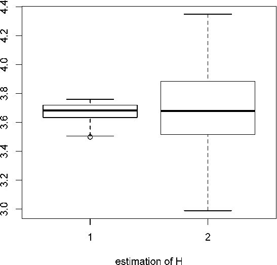
Figure 5.4. (a) Curve drawing reflectance in function of wavelength, varying between 11001100 and 24982498. (b) Box-plots for both estimators on the left H^n(1)\widehat{H}_{n}^{(1)}, on the right H^n(2)\widehat{H}_{n}^{(2)} for the 3939 curves and (u,v)=(1,4)(u,v)=(1,4).
Table 5.9. Means of estimates in the biscuit example
m=2m=2 m=4m=4 m=6m=6 m=8m=8 m=10m=10
H^n(1)\widehat{H}_{n}^{(1)} 3.60 (0.12) 3.67 (0.07) 3.65 (0.05) 3.62 (0.04) 3.59 (0.04)
αOLS(1)\alpha^{(1)}_{\text{OLS}} 3.60 (0.12) 3.67 (0.07) 3.66 (0.05) 3.63 (0.04) 3.60 (0.03)
H^n(2)\widehat{H}_{n}^{(2)} 2.84 (0.45) 3.69 (0.30) 3.83 (0.24) 3.84 (0.19) 3.83 (0.16)
αOLS(2)\alpha^{(2)}_{\text{OLS}} 2.84 (0.45) 3.67 (0.31) 3.91 (0.23) 3.98 (0.18) 3.99 (0.14)

Now, in order to compare the (empirical) variances of these estimators, we consider a second example introduced by Brown et al. (2001). The experiment involved varying the composition of biscuit dough pieces and data consist in near infrared reflectance (NIR) spectra for the same dough. The 40 curves are graphed on the figure 5.4. Each represents the near-infrared spectrum reflectance measure at each 22 nanometers from 11001100 to 24982498 nm, then 700700 observation points for each biscuit. According to Brown et al. (2001), the observation 23 appears as an outlier. We estimate r0r_{\scriptscriptstyle 0} for each of the left 39 curves, using the threshold bn=1b_{n}=1, which gives r^0=1\widehat{r}_{\scriptscriptstyle 0}=1 for each curve. Furthermore, the averaged mean quadratic variation n2​r−2​(Dr(1)​X)2¯n^{2r-2}\overline{\big(D_{r}^{(1)}X\big)^{2}} equals to 0.330.33 when r=2r=2 and 122133122133 when r=3r=3, this explosion confirming the choice r0^=3−2=1\widehat{r_{\scriptscriptstyle 0}}=3-2=1. We turn to estimation of HH, having in mind the comparison of our estimators together with αOLS(p)\alpha_{\text{OLS}}^{(p)} (where p=1p=1 corresponds to the choice (1,−2,1)(1,-2,1) for aj​ra_{jr} and p=2p=2 to the choice (−1,3,−3,1)(-1,3,-3,1)). The results are summarized in Table 5.9 where it appears that, for order r0^+2=3\widehat{r_{\scriptscriptstyle 0}}+2=3, our estimator H^n(2)\widehat{H}_{n}^{(2)} seems to be less sensitive toward high values of mm. Also our simplified estimators present a similar variance to α^O​L​S(p)\widehat{\alpha}_{OLS}^{(p)}, p=1,2p=1,2. To conclude this part, it should be noticed that for the 23rd curve, the choice m=4m=4 gives H^n(1)=3.64\widehat{H}_{n}^{(1)}=3.64 and H^n(2)=3.55\widehat{H}_{n}^{(2)}=3.55. It appears that, in both cases, these values belong to the interquartile range obtained from the 39 curves, so at least concerning the regularity, the curve 23 should not be considered as an outlier.

6. Annexes

6.1. Proofs of section 2

Lemma 6.1.

Let YY be a zero mean process with given regularity (r0,β0)(r_{\scriptscriptstyle 0},\beta_{\scriptscriptstyle 0}) and asymptotic function d0​(t)≡Cr0,β0d_{0}(t)\equiv C_{r_{\scriptscriptstyle 0},\beta_{\scriptscriptstyle 0}} that satisfies A2.1(iii-pp) (p=1p=1 or 2). For a positive function a∈Cr0+p​([0,T])a\in C^{r_{\scriptscriptstyle 0}+p}([0,T]) and m∈Cr0+p​([0,T])m\in C^{r_{\scriptscriptstyle 0}+p}([0,T]), if X⁡(t)=a⁡(t)​Y​(t)+m⁡(t)X(t)=a(t)Y(t)+m(t), then XX has regularity (r0,β0)(r_{\scriptscriptstyle 0},\beta_{\scriptscriptstyle 0}) with asymptotical function Dr0,β0​(t)=a2​(t)​Cr0,β0D_{r_{\scriptscriptstyle 0},\beta_{\scriptscriptstyle 0}}(t)=a^{2}(t)C_{r_{\scriptscriptstyle 0},\beta_{\scriptscriptstyle 0}} and satisfies A2.1(iii-pp).

Proof.

See Seleznjev (2000) and straightforward computation. ∎

Lemma 6.2.

Under Assumptions A2.2, we get for k=0,…,n−1k=0,\dotsc,n-1, and i=1,…,n−ki=1,\dotsc,n-k:

(6.1) tk+i−tk\displaystyle t_{k+i}-t_{k} ≥C1​i​δn,C1=(T​supt∈[0,T]ψ⁡(t))−1,\displaystyle\geq C_{1}i\delta_{n},\;\;C_{1}=(T\sup_{t\in[0,T]}\psi(t))^{-1},
(6.2) tk+i−tk\displaystyle t_{k+i}-t_{k} ≤C2​i​δn,C2=(T​inft∈[0,T]ψ⁡(t))−1,\displaystyle\leq C_{2}i\delta_{n},\;\;C_{2}=(T\inf_{t\in[0,T]}\psi(t))^{-1},
and if i=1,…,imaxi=1,\dotsc,i_{\max} with imaxi_{\max} not depending on nn:
(6.3) tk+i−tk\displaystyle t_{k+i}-t_{k} =i​δnT​ψ​(tk)​(1+𝒪⁡(δnα))\displaystyle=\frac{i\delta_{n}}{T\psi(t_{k})}(1+{\cal O}(\delta_{n}^{\alpha}))

where 𝒪⁡(…){\cal O}(\dots) is uniform over ii and kk.

Proof.

Relations (6.1)-(6.2) are obtained with the mean-value theorem that induces, for k=0,…,n−1k=0,\dotsc,n-1 and i=1,…,n−ki=1,\dotsc,n-k:

tk+i−tk=i​δnT​ψ​(tk+θ⁡(tk+i−tk)),  0<θ<1.t_{k+i}-t_{k}=\frac{i\delta_{n}}{T\psi(t_{k}+\theta(t_{k+i}-t_{k}))},\;\;0<\theta<1.

To obtain the equivalence (6.3), one may write tk+i−tk=i​δnT​ψ​(tk)​(1+Rn)t_{k+i}-t_{k}=\frac{i\delta_{n}}{T\psi(t_{k})}(1+R_{n}) with RnR_{n} defined by

Rn=ψ⁡(tk)−ψ⁡(tk+θ⁡(tk+i−tk))ψ⁡(tk+θ⁡(tk+i−tk))≤L​|tk+i−tk|αinft∈[0,T]ψ⁡(t)=𝒪⁡(δnα)R_{n}=\frac{\psi(t_{k})-\psi(t_{k}+\theta(t_{k+i}-t_{k}))}{\psi(t_{k}+\theta(t_{k+i}-t_{k}))}\leq\frac{L\left|t_{k+i}-t_{k}\right|^{\alpha}}{\inf_{t\in[0,T]}\psi(t)}={\cal O}(\delta_{n}^{\alpha})

by Assumption A2.2 and uniformly over ii, nn and kk for i=1,…,imaxi=1,\dotsc,i_{\max}. ∎

Lemma 6.3.

We have under Assumption A2.2 and for r≥1r\geq 1, i=0,…,ri=0,\dotsc,r,

  1. (1)

    for p=0,…,r−1p=0,\dotsc,r-1 and convention 00=10^{0}=1

    (6.4) ∑i=0r(tk+i​u−tk)p​bi​k​r(u)=0,\sum_{i=0}^{r}(t_{k+iu}-t_{k})^{p}b_{ikr}^{(u)}=0,
  2. (2)
    (6.5) ∑i=0r(tk+i​u−tk)r​bi​k​r(u)=1,\sum_{i=0}^{r}(t_{k+iu}-t_{k})^{r}b_{ikr}^{(u)}=1,
  3. (3)
    (6.6) |bi​k​r(u)|≤C1−r​u−r​δn−r,∏m=0,m≠ir|i−m|,\left|b_{ikr}^{(u)}\right|\leq\frac{C_{1}^{-r}u^{-r}\delta_{n}^{-r},}{\prod_{m=0,m\not=i}^{r}\left|i-m\right|},

    with C1C_{1} given by (6.1),

  4. (4)
    (6.7) bi​k​r(u)=u−r​ψr​(tk)​Tr​δn−r∏m=0,m≠ir(i−m)​(1+𝒪⁡(δnα))b_{ikr}^{(u)}=\frac{u^{-r}\psi^{r}(t_{k})T^{r}\delta_{n}^{-r}}{\prod_{m=0,m\not=i}^{r}(i-m)}(1+{\cal O}(\delta_{n}^{\alpha}))

    with 𝒪⁡(…){\cal O}(\dots) uniform over ii and kk.

Proof.

The term g⁡[tk,…,tk+r​u]=∑i=0rbi​k​r(u)​g​(tk+i​u)g[t_{k},\dotsc,t_{k+ru}]=\sum_{i=0}^{r}b_{ikr}^{(u)}g(t_{k+iu}) is the leading coefficient in the polynomial approximation of degree rr of gg, given in the decomposition (2.2). Considering the polynomial g⁡(t)=(t−tk)pg(t)=(t-t_{k})^{p}, we may immediately deduce the properties (6.4)-(6.5), from uniqueness of relation (2.2). Next, (6.6)-(6.7) are direct consequences of Lemma 6.2 and definition (2.3) of bi​k​r(u)b_{ikr}^{(u)}. ∎

Proposition 6.1.

Under Assumption A2.1 and A2.2, one obtains:
(i) for r=r0+pr=r_{\scriptscriptstyle 0}+p with p=1,2p=1,2:

n−2​(p−β0)​𝔼​((Dr0+p(u)​X)2¯)→n→∞u−2​(p−β0)​ℓ​(p,r0,β0)n^{-2(p-\beta_{\scriptscriptstyle 0})}\,\mathds{E}\Big(\,\overline{\big(D_{r_{\scriptscriptstyle 0}+p}^{(u)}X\big)^{2}}\,\Big)\xrightarrow[n\to\infty]{}u^{-2(p-\beta_{\scriptscriptstyle 0})}\ell(p,r_{\scriptscriptstyle 0},\beta_{\scriptscriptstyle 0})

where ℓ(p,0,β0)=−12∫0Td0(t)ψ2​p+1​(t)ψ2​β0​(t)dt∑i,j=0p|i−j|2​β0∏m=0m≠ip(i−m)​∏q=0q≠jp(j−q)\displaystyle\ell(p,0,\beta_{\scriptscriptstyle 0})=-\frac{1}{2}\int_{0}^{T}d_{0}(t)\frac{\psi^{2p+1}(t)}{\psi^{2\beta_{\scriptscriptstyle 0}}(t)}\,{\mathrm{d}}t\sum_{i,j=0}^{p}\frac{\left|i-j\right|^{2\beta_{\scriptscriptstyle 0}}}{\prod_{\begin{subarray}{c}m=0\\ m\not=i\end{subarray}}^{p}(i-m)\prod_{\begin{subarray}{c}q=0\\ q\not=j\end{subarray}}^{p}(j-q)} while if r0≥1r_{\scriptscriptstyle 0}\geq 1,

(6.8) ℓ⁡(p,r0,β0)=(−1)r0+1​∫0Td0​(t)​ψ2​p+1​(t)ψ2​β0​(t)​𝑑t2​(2​β0+2​r0)​⋯​(2​β0+1)​∑i,j=0r0+p|i−j|2​(r0+β0)∏m=0m≠ir0+p(i−m)​∏q=0q≠jr0+p(j−q)\ell(p,r_{\scriptscriptstyle 0},\beta_{\scriptscriptstyle 0})=\frac{(-1)^{r_{\scriptscriptstyle 0}+1}\int_{0}^{T}d_{0}(t)\frac{\psi^{2p+1}(t)}{\psi^{2\beta_{\scriptscriptstyle 0}}(t)}\,{\mathrm{d}}t}{2(2\beta_{\scriptscriptstyle 0}+2r_{\scriptscriptstyle 0})\dotsm(2\beta_{\scriptscriptstyle 0}+1)}\sum_{i,j=0}^{r_{\scriptscriptstyle 0}+p}\frac{\left|i-j\right|^{2(r_{\scriptscriptstyle 0}+\beta_{\scriptscriptstyle 0})}}{\prod_{\begin{subarray}{c}m=0\\ m\not=i\end{subarray}}^{r_{\scriptscriptstyle 0}+p}(i-m)\prod_{\begin{subarray}{c}q=0\\ q\not=j\end{subarray}}^{r_{\scriptscriptstyle 0}+p}(j-q)}

(ii) for r0≥1r_{\scriptscriptstyle 0}\geq 1 and r=1,…,r0r=1,\dotsc,r_{\scriptscriptstyle 0}:

𝔼⁡((Dr(u)​X)2¯)→n→∞1(r!)2​∫0T𝔼​(X(r)​(t))2​ψ​(t)​𝑑t.\mathds{E}\Big(\,\overline{\big(D_{r}^{(u)}X\big)^{2}}\,\Big)\xrightarrow[n\to\infty]{}\frac{1}{(r!)^{2}}\int_{0}^{T}\mathds{E}\big(X^{(r)}(t)\big)^{2}\psi(t)\,{\mathrm{d}}t.
Proof.

A. Let us begin with general expressions of 𝔼⁡(Dr,k(u)​X​Dr,ℓ(u)​X)\displaystyle\mathds{E}\Big(\,D_{r,k}^{(u)}\,XD_{r,\ell}^{(u)}\,X\Big) useful for the sequel. First for 𝕃(p,p)​(s,t)=𝔼⁡(X(p)​(s)​X(p)​(t))\mathds{L}^{(p,p)}(s,t)=\mathds{E}\big(X^{(p)}(s)X^{(p)}(t)\big) (p≥0p\geq 0), the relation (2.1) is equivalent to

(6.9) limh→0sups,t∈[0,T]|s−t|≤h,s≠t|𝕃(r0,r0)​(s,s)+𝕃(r0,r0)​(t,t)−2​𝕃(r0,r0)​(s,t)|s−t|2​β0−d0​(t)|=0.\lim_{h\to 0}\sup_{\begin{subarray}{c}s,t\in[0,T]\\ \left|s-t\right|\leq h,s\not=t\end{subarray}}\left|\frac{\mathds{L}^{(r_{\scriptscriptstyle 0},r_{\scriptscriptstyle 0})}(s,s)+\mathds{L}^{(r_{\scriptscriptstyle 0},r_{\scriptscriptstyle 0})}(t,t)-2\mathds{L}^{(r_{\scriptscriptstyle 0},r_{\scriptscriptstyle 0})}(s,t)}{\left|s-t\right|^{2\beta_{\scriptscriptstyle 0}}}-d_{0}(t)\right|=0.

For (v,w)∈[0,1]2(v,w)\in[0,1]^{2}, we set v˙i​k=tk+(tk+i​u−tk)​v\dot{v}_{ik}=t_{k}+(t_{k+iu}-t_{k})v and w˙j​ℓ=tℓ+(tℓ+j​u−tℓ)​w\dot{w}_{j\ell}=t_{\ell}+(t_{\ell+ju}-t_{\ell})w. Next, from the definition of Dr,k(u)​XD_{r,k}^{(u)}\,X given in (2.4), we get

𝔼⁡(Dr,k(u)​X​Dr,ℓ(u)​X)=∑i,j=0rbi​k​r(u)​bj​ℓ​r(u)​𝕃(0,0)​(tk+i​u,tℓ+j​u).\mathds{E}(D_{r,k}^{(u)}\,XD_{r,\ell}^{(u)}\,X)=\sum\limits_{i,j=0}^{r}b_{ikr}^{(u)}b_{j\ell r}^{(u)}\mathds{L}^{(0,0)}(t_{k+iu},t_{\ell+ju}).

For r0=0r_{\scriptscriptstyle 0}=0 and since ∑i=0rbi​k​r(u)=0\sum_{i=0}^{r}b_{ikr}^{(u)}=0, we have:

(6.10) 𝔼(Dr,k(u)XDr,ℓ(u)X)=∑i,j=0rbi​k​r(u)bj​ℓ​r(u){𝕃(0,0)(tk+i​u,tℓ+j​u)−12𝕃(0,0)(tk+i​u,tk+i​u)−12𝕃(0,0)(tℓ+j​u,tℓ+j​u)}.\mathds{E}(D_{r,k}^{(u)}\,XD_{r,\ell}^{(u)}\,X)=\sum_{i,j=0}^{r}\!b_{ikr}^{(u)}b_{j\ell r}^{(u)}\Big\{\mathds{L}^{(0,0)}(t_{k+iu},t_{\ell+ju})\\ -\frac{1}{2}\mathds{L}^{(0,0)}(t_{k+iu},t_{k+iu})-\frac{1}{2}\mathds{L}^{(0,0)}(t_{\ell+ju},t_{\ell+ju})\Big\}.

If r0≥1r_{\scriptscriptstyle 0}\geq 1, we apply multiple Taylor series expansions with integral remainder. Next, the properties ∑i=0rbi​k​r(u)​(tk+i​u−tk)p=0\sum_{i=0}^{r}b_{ikr}^{(u)}(t_{k+iu}-t_{k})^{p}=0 for p=0,…,r−1p=0,\dotsc,r-1 (and convention 00=10^{0}=1) induce :

(6.11) 𝔼⁡(Dr,k(u)​X​Dr,ℓ(u)​X)=∑i,j=0rbi​k​r(u)​bj​ℓ​r(u)​(tk+i​u−tk)r∗​(tℓ+j​u−tℓ)r∗×∫∫[0,1]2(1−v)r∗−1​(1−w)r∗−1((r∗−1)!)2​𝕃(r∗,r∗)​(v˙i​k,w˙j​ℓ)​𝑑v​𝑑w\mathds{E}(D_{r,k}^{(u)}\,XD_{r,\ell}^{(u)}\,X)=\sum_{i,j=0}^{r}\!b_{ikr}^{(u)}b_{j\ell r}^{(u)}(t_{k+iu}-t_{k})^{r^{\ast}}(t_{\ell+ju}-t_{\ell})^{r^{\ast}}\\ \times\int\!\!\!\int_{[0,1]^{2}}\!\frac{\!(1-v)^{r^{\ast}-1}\!(1-w)^{r^{\ast}-1}}{((r^{\ast}-1)!)^{2}}\mathds{L}^{(r^{\ast},r^{\ast})}(\dot{v}_{ik},\dot{w}_{j\ell})\,{\mathrm{d}}v\!\,{\mathrm{d}}w

where we have set r∗=min⁡(r0,r)≥1r^{\ast}=\min(r_{\scriptscriptstyle 0},r)\geq 1.

B. From expressions (6.10)-(6.11), we are in position to derive the asymptotic behavior of 𝔼⁡((Dr(u)​X)2¯)\mathds{E}\big(\,\overline{(D_{r}^{(u)}\,X)^{2}}\big).

Case r0≥1r_{\scriptscriptstyle 0}\geq 1, r=r0+pr=r_{\scriptscriptstyle 0}+p, p=1p=1 or p=2p=2.

In this case, r∗=r0≤r−1r^{\ast}=r_{\scriptscriptstyle 0}\leq r-1. From (6.11) and the property ∑i=0rbi​k​r(u)​(tk+i​u−tk)r0=0\sum_{i=0}^{r}b_{ikr}^{(u)}(t_{k+iu}-t_{k})^{r_{\scriptscriptstyle 0}}=0, we may write

(6.12) 𝔼​(Dr,k(u)​X)2=∑i,j=0rbi​k​r(u)​bj​k​r(u)​(tk+i​u−tk)r0​(tk+j​u−tk)r0​∫01∫01((1−v)​(1−w))r0−1((r0−1)!)2×{𝕃(r0,r0)​(v˙i​k,w˙j​k)−12​𝕃(r0,r0)​(v˙i​k,v˙i​k)−12​𝕃(r0,r0)​(w˙j​k,w˙j​k)}​d​v​d​w\mathds{E}(D_{r,k}^{(u)}\,X)^{2}=\sum_{i,j=0}^{r}b_{ikr}^{(u)}b_{jkr}^{(u)}(t_{k+iu}-t_{k})^{r_{\scriptscriptstyle 0}}(t_{k+ju}-t_{k})^{r_{\scriptscriptstyle 0}}\!\!\int_{0}^{1}\!\!\!\int_{0}^{1}\!\!\frac{((1-v)(1-w))^{r_{\scriptscriptstyle 0}-1}}{((r_{\scriptscriptstyle 0}-1)!)^{2}}\\ \times\Big\{\mathds{L}^{(r_{\scriptscriptstyle 0},r_{\scriptscriptstyle 0})}(\dot{v}_{ik},\dot{w}_{jk})-\frac{1}{2}\mathds{L}^{(r_{\scriptscriptstyle 0},r_{\scriptscriptstyle 0})}(\dot{v}_{ik},\dot{v}_{ik})-\frac{1}{2}\mathds{L}^{(r_{\scriptscriptstyle 0},r_{\scriptscriptstyle 0})}(\dot{w}_{jk},\dot{w}_{jk})\Big\}\,{\mathrm{d}}v\!\,{\mathrm{d}}w

Using the locally stationary condition (6.9), uniform continuity of d0​(⋅)d_{0}(\cdot) on [0,T][0,T] and the bound: |v˙i​k−w˙j​k|≤tk+r​u−tk≤C1​r​u​δn\left|\dot{v}_{ik}-\dot{w}_{jk}\right|\leq t_{k+ru}-t_{k}\leq C_{1}ru\delta_{n} for i=0,…,ri=0,\dotsc,r and j=0,…,rj=0,\dotsc,r, we may show that the predominant term for 𝔼⁡((Dr(u)​X)2¯)\mathds{E}\big(\,\overline{(D_{r}^{(u)}\,X)^{2}}\big) is given by:

(6.13) −12​(nr+1)​∑k=0nr∑i,j=0rbi​k​r(u)​bj​k​r(u)​(tk+i​u−tk)r0​(tk+j​u−tk)r0×∫∫[0,1]2((1−v)​(1−w))r0−1((r0−1)!)2​|v˙i​k−w˙j​k|2​β0​d0​(tk)​dv​dw.\frac{-1}{2(n_{r}+1)}\sum_{k=0}^{n_{r}}\sum_{i,j=0}^{r}b_{ikr}^{(u)}b_{jkr}^{(u)}(t_{k+iu}-t_{k})^{r_{\scriptscriptstyle 0}}(t_{k+ju}-t_{k})^{r_{\scriptscriptstyle 0}}\\ \times\int\!\!\!\int_{[0,1]^{2}}\frac{((1-v)(1-w))^{r_{\scriptscriptstyle 0}-1}}{((r_{\scriptscriptstyle 0}-1)!)^{2}}\left|\dot{v}_{ik}-\dot{w}_{jk}\right|^{2\beta_{\scriptscriptstyle 0}}d_{0}(t_{k})\,{\mathrm{d}}v\,{\mathrm{d}}w.

From the equivalents (6.3) and (6.7), we can write the leading term of (6.13) as a Riemann sum on tkt_{k} to obtain

δn2​p−2​β0𝔼((Dr(u)​X)2¯)→n→∞−12(uT)−2​p+2​β0∫0Td0(t)ψ2​p+1−2​β0(t)dt×∑i,j=0r(i​j)r0∏m=0m≠ir(i−m)​∏q=0q≠jr(j−q)​∫∫[0,1]2((1−v)​(1−w))r0−1((r0−1)!)2​|i​v−j​w|2​β0​dv​dw.\delta_{n}^{2p-2\beta_{\scriptscriptstyle 0}}\mathds{E}\big(\,\overline{(D_{r}^{(u)}\,X)^{2}}\big)\xrightarrow[n\to\infty]{}-\frac{1}{2}(\frac{u}{T})^{-2p+2\beta_{\scriptscriptstyle 0}}\int_{0}^{T}d_{0}(t)\psi^{2p+1-2\beta_{\scriptscriptstyle 0}}(t)\,{\mathrm{d}}t\\ \times\sum_{i,j=0}^{r}\frac{(ij)^{r_{\scriptscriptstyle 0}}}{\prod\limits_{\begin{subarray}{c}m=0\\ m\not=i\end{subarray}}^{r}(i-m)\prod\limits_{\begin{subarray}{c}q=0\\ q\not=j\end{subarray}}^{r}(j-q)}\int\!\!\!\int_{[0,1]^{2}}\!\!\frac{((1-v)(1-w))^{r_{\scriptscriptstyle 0}-1}}{((r_{\scriptscriptstyle 0}-1)!)^{2}}\left|iv-jw\right|^{2\beta_{\scriptscriptstyle 0}}\,{\mathrm{d}}v\,{\mathrm{d}}w.

Next by performing elementary but tedious multiple integrations by parts, we arrive at the following simpler form of ℓ⁡(r,r0,β0)\ell(r,r_{\scriptscriptstyle 0},\beta_{\scriptscriptstyle 0}) given in (6.8), for n​δn→Tn\delta_{n}\to T.

Case r0=0r_{\scriptscriptstyle 0}=0, r=r0+1,,r0+2r=r_{\scriptscriptstyle 0}+1,_{,}r_{\scriptscriptstyle 0}+2.

The proof is the same but starting from (6.10) and ℓ=k\ell=k.

Case r0≥1r_{\scriptscriptstyle 0}\geq 1 and r=1,…,r0r=1,\dotsc,r_{\scriptscriptstyle 0}.

In this case, r∗=rr^{\ast}=r and from the relation (6.11), one gets

𝔼​(Dr,k(u)​X)2=∑i,j=0rbi​k​r(u)​bj​k​r(u)​(tk+i​u−tk)r​(tk+j​u−tk)r×∫∫[0,1]2((1−v)​(1−w))r−1((r−1)!)2​𝕃(r,r)​(v˙i​k,w˙j​k)​dv​dw.\mathds{E}(D_{r,k}^{(u)}\,X)^{2}=\sum\limits_{i,j=0}^{r}\!b_{ikr}^{(u)}b_{jkr}^{(u)}(t_{k+iu}-t_{k})^{r}(t_{k+ju}-t_{k})^{r}\\ \times\int\!\!\!\int_{[0,1]^{2}}\frac{((1-v)(1-w))^{r-1}}{((r-1)!)^{2}}\mathds{L}^{(r,r)}(\dot{v}_{ik},\dot{w}_{jk})\,{\mathrm{d}}v\!\,{\mathrm{d}}w.

The result follows after Riemann summation with the help of uniform continuity of 𝕃(r,r)​(⋅,⋅)\mathds{L}^{(r,r)}(\cdot,\cdot), r=1,…,r0r=1,\dotsc,r_{\scriptscriptstyle 0} and properties (6.3), (6.5). ∎

6.2. Auxiliary results

The following lemma gives some useful results on the asymptotic behavior of ℂr​(k,ℓ)\mathds{C}_{r}(k,\ell) and ℂr2​(k,ℓ)\mathds{C}_{r}^{2}(k,\ell) with ℂr​(k,ℓ)=Cov⁡(Dr,k(u)​X,Dr,ℓ(u)​X)\mathds{C}_{r}(k,\ell)={\mathrm{Cov\,}}\big(D_{r,k}^{(u)}\,X,D_{r,\ell}^{(u)}\,X\big) with nr=n−u​rn_{r}=n-ur and uu a positive integer.

Lemma 6.4.

Suppose that Assumption A2.1 and A2.2 are fulfilled.

(i) Under the condition A2.1-(iii-1) and for r=r0+pr=r_{\scriptscriptstyle 0}+p, p=1p=1 or p=2p=2, one obtains

max⁡∑ℓ=0nrk=0,…,nr⁡|ℂr​(k,ℓ)|={𝒪⁡(n2​p−2​β0) if ​0<β0<12,𝒪⁡(n2​p−1​ln⁡n) if ​β0=12,𝒪⁡(n2​p−1) if ​12<β0<1;\max_{k=0,\dotsc,n_{r}}\sum_{\ell=0}^{n_{r}}\left|\mathds{C}_{r}(k,\ell)\right|=\begin{cases}{\mathcal{O}}(n^{2p-2\beta_{\scriptscriptstyle 0}})&\text{ if }0<\beta_{\scriptscriptstyle 0}<\frac{1}{2},\\ {\mathcal{O}}(n^{2p-1}\ln n)&\text{ if }\beta_{\scriptscriptstyle 0}=\frac{1}{2},\\ {\mathcal{O}}(n^{2p-1})&\text{ if }\frac{1}{2}<\beta_{\scriptscriptstyle 0}<1\penalty\ ;\end{cases}

and

∑k=0nr∑ℓ=0nrℂr2​(k,ℓ)={𝒪⁡(n4​p−4​β0+1) if ​0<β0<34,𝒪⁡(n4​p−2​ln⁡n) if ​β0=34,𝒪⁡(n4​p−2) if ​34<β0<1.\sum_{k=0}^{n_{r}}\sum_{\ell=0}^{n_{r}}\mathds{C}_{r}^{2}(k,\ell)=\begin{cases}{\mathcal{O}}(n^{4p-4\beta_{\scriptscriptstyle 0}+1})&\text{ if }0<\beta_{\scriptscriptstyle 0}<\frac{3}{4},\\ {\mathcal{O}}(n^{4p-2}\ln n)&\text{ if }\beta_{\scriptscriptstyle 0}=\frac{3}{4},\\ {\mathcal{O}}(n^{4p-2})&\text{ if }\frac{3}{4}<\beta_{\scriptscriptstyle 0}<1.\end{cases}

(ii) Under the condition A2.1-(iii-2) and for r=r0+2r=r_{\scriptscriptstyle 0}+2, one obtains

max⁡∑ℓ=0nrk=0,…,nr⁡|ℂr​(k,ℓ)|=𝒪⁡(n4−2​β0)​ and ​∑k=0nr∑ℓ=0nrℂr2​(k,ℓ)=𝒪⁡(n9−4​β0).\max\limits_{k=0,\dotsc,n_{r}}\sum_{\ell=0}^{n_{r}}\left|\mathds{C}_{r}(k,\ell)\right|={\mathcal{O}}(n^{4-2\beta_{\scriptscriptstyle 0}})\text{ and }\sum_{k=0}^{n_{r}}\sum_{\ell=0}^{n_{r}}\mathds{C}_{r}^{2}(k,\ell)={\mathcal{O}}(n^{9-4\beta_{\scriptscriptstyle 0}}).

(iii) If r=1,…,r0r=1,\dotsc,r_{\scriptscriptstyle 0} (with r0≥1r_{\scriptscriptstyle 0}\geq 1), then max⁡∑ℓ=0nrk=0,…,nr⁡|ℂr​(k,ℓ)|=𝒪⁡(n)\displaystyle\max_{k=0,\dotsc,n_{r}}\sum_{\ell=0}^{n_{r}}\left|\mathds{C}_{r}(k,\ell)\right|={\mathcal{O}}(n) and ∑k=0nr∑ℓ=0nrℂr2​(k,ℓ)=𝒪⁡(n2).\displaystyle\sum_{k=0}^{n_{r}}\sum_{\ell=0}^{n_{r}}\mathds{C}_{r}^{2}(k,\ell)={\mathcal{O}}(n^{2}).

Proof.

(i) Setting μ⁡(t)=𝔼⁡(X⁡(t))\mu(t)=\mathds{E}\big(X(t)\big), μ\mu is r0r_{\scriptscriptstyle 0}-times differentiable and similarly to (6.10)-(6.11), we get the expansion

ℂr​(k,ℓ)=∑i,j=0rbi​k​r(u)​bj​ℓ​r(u)​(tk+i​u−tk)r0​(tℓ+j​u−tℓ)r0×∫∫[0,1]2((1−v)​(1−w))r0−1((r0−1)!)2​𝕂(r0,r0)​(v˙i​k,w˙j​ℓ)​𝑑v​𝑑w\mathds{C}_{r}(k,\ell)=\sum_{i,j=0}^{r}b_{ikr}^{(u)}b_{j\ell r}^{(u)}(t_{k+iu}-t_{k})^{r_{\scriptscriptstyle 0}}(t_{\ell+ju}-t_{\ell})^{r_{\scriptscriptstyle 0}}\\ \times\int\!\!\!\int_{[0,1]^{2}}\frac{((1-v)(1-w))^{r_{\scriptscriptstyle 0}-1}}{((r_{\scriptscriptstyle 0}-1)!)^{2}}\mathds{K}^{(r_{\scriptscriptstyle 0},r_{\scriptscriptstyle 0})}(\dot{v}_{ik},\dot{w}_{j\ell})\,{\mathrm{d}}v\,{\mathrm{d}}w

for r0≥1r_{\scriptscriptstyle 0}\geq 1 while if r0=0r_{\scriptscriptstyle 0}=0, ℂr​(k,ℓ)=∑i=0r∑j=0rbi​k​r(u)​bj​ℓ​r(u)​𝕂​(tk+i​u,tℓ+j​u)\mathds{C}_{r}(k,\ell)=\sum_{i=0}^{r}\sum_{j=0}^{r}b_{ikr}^{(u)}b_{j\ell r}^{(u)}\mathds{K}(t_{k+iu},t_{\ell+ju}).

Case r=r0+1r=r_{\scriptscriptstyle 0}+1 or r0+2r_{\scriptscriptstyle 0}+2.

For r0≥1r_{\scriptscriptstyle 0}\geq 1, we have the bound:

max⁡∑ℓ=0nrk=0,…,nr⁡|ℂr​(k,ℓ)|≤U1​n+U2​n+U3​n\max_{k=0,\dotsc,n_{r}}\sum_{\ell=0}^{n_{r}}\left|\mathds{C}_{r}(k,\ell)\right|\leq U_{1n}+U_{2n}+U_{3n}

with U1​n=max⁡∑ℓ=0k−u​r−1k=u​r+1,…,nr⁡|ℂr​(k,ℓ)|U_{1n}=\max\limits_{k=ur+1,\dotsc,n_{r}}\sum\limits_{\ell=0}^{k-ur-1}\!\!\left|\mathds{C}_{r}(k,\ell)\right|, U2​n=max⁡∑ℓ=k+u​r+1nrk=0,…,n−2​u​r−1⁡|ℂr​(k,ℓ)|U_{2n}=\max\limits_{k=0,\dotsc,n-2ur-1}\sum\limits_{\ell=k+ur+1}^{n_{r}}\!\!\left|\mathds{C}_{r}(k,\ell)\right| and U3​n=max⁡∑ℓ=max⁡(0,k−u​r)min⁡(nr,k+u​r)k=0,…,nr⁡|ℂr​(k,ℓ)|U_{3n}=\max\limits_{k=0,\dotsc,n_{r}}\sum\limits_{\ell=\max(0,k-ur)}^{\min(n_{r},k+ur)}\left|\mathds{C}_{r}(k,\ell)\right|. First, consider the sum U1​n+U2​nU_{1n}+U_{2n} where |k−ℓ|≥u​r+1\left|k-\ell\right|\geq ur+1. Since ∑i=0rbi​k​r(u)​(tk+i​u−tk)r0=0\sum_{i=0}^{r}b_{ikr}^{(u)}(t_{k+iu}-t_{k})^{r_{\scriptscriptstyle 0}}=0 for r=r0+1r=r_{\scriptscriptstyle 0}+1 or r=r0+2r=r_{\scriptscriptstyle 0}+2, and [tk,v˙i​k][t_{k},\dot{v}_{ik}] is distinct from [tℓ,w˙j​ℓ][t_{\ell},\dot{w}_{j\ell}], we get

(6.14) ℂr​(k,ℓ)=∑i,j=0rbi​k​r(u)​bj​k​r(u)​(tk+i​u−tk)r0​(tℓ+j​u−tℓ)r0×∫∫[0,1]2((1−v)​(1−w))r0−1((r0−1)!)2​∫tkv˙i​k∫tℓw˙j​ℓ𝕂(r0+1,r0+1)​(s,t)​ds​dt​dv​dw.\mathds{C}_{r}(k,\ell)=\sum_{i,j=0}^{r}b_{ikr}^{(u)}b_{jkr}^{(u)}(t_{k+iu}-t_{k})^{r_{\scriptscriptstyle 0}}(t_{\ell+ju}-t_{\ell})^{r_{\scriptscriptstyle 0}}\\ \times\int\!\!\!\int_{[0,1]^{2}}\frac{((1-v)(1-w))^{r_{\scriptscriptstyle 0}-1}}{((r_{\scriptscriptstyle 0}-1)!)^{2}}\int_{t_{k}}^{\dot{v}_{ik}}\int_{t_{\ell}}^{\dot{w}_{j\ell}}\mathds{K}^{(r_{\scriptscriptstyle 0}+1,r_{\scriptscriptstyle 0}+1)}(s,t)\,\mathrm{d}s\!\,{\mathrm{d}}t\!\,{\mathrm{d}}v\!\,{\mathrm{d}}w.

Condition A2.1-(iii-1), together with the bounds (6.2) and (6.6), gives a bound of 𝒪⁡(n2​p−2​β0​∑i=1ni−2​(1−β0)){\mathcal{O}}(n^{2p-2\beta_{\scriptscriptstyle 0}}\sum_{i=1}^{n}i^{-2(1-\beta_{\scriptscriptstyle 0})}) for |U1​n+U2​n|\left|U_{1n}+U_{2n}\right|, which is of order n2​(p−β0)n^{2(p-\beta_{\scriptscriptstyle 0})} if 0<β0<120<\beta_{\scriptscriptstyle 0}<\frac{1}{2}, n2​(p−β0)​ln⁡nn^{2(p-\beta_{\scriptscriptstyle 0})}\ln n if β0=12\beta_{\scriptscriptstyle 0}=\frac{1}{2} and n2​p−1n^{2p-1} if β0>12\beta_{\scriptscriptstyle 0}>\frac{1}{2}. Next, for U3​nU_{3n} where |k−ℓ|≤u​r\left|k-\ell\right|\leq ur, we obtain that U3​n=𝒪⁡(n2​(p−β0))U_{3n}={\cal O}(n^{2(p-\beta_{\scriptscriptstyle 0})}) in a similar way as in the proof of Proposition 6.1, and with the help of Cauchy-Schwarz inequality to control the terms depending on μ(r0)​(t)\mu^{(r_{\scriptscriptstyle 0})}(t).

We proceed similarly for the case r0=0r_{\scriptscriptstyle 0}=0, starting from the definition of ℂr​(k,ℓ)\mathds{C}_{r}(k,\ell) as well as for the study of ∑k=0nr∑ℓ=0nrℂr2​(k,ℓ)\sum_{k=0}^{n_{r}}\sum_{\ell=0}^{n_{r}}\mathds{C}_{r}^{2}(k,\ell) for which dominant terms are of order 𝒪⁡(n1+4​p−4​β0​∑i=1ni−4​(1−β0)){\cal O}(n^{1+4p-4\beta_{\scriptscriptstyle 0}}\sum_{i=1}^{n}i^{-4(1-\beta_{\scriptscriptstyle 0})}).

(ii) The condition A2.1-(iii-2) and r=r0+2r=r_{\scriptscriptstyle 0}+2 allows to transform (6.14) into

(6.15) ℂr​(k,ℓ)=∑i,j=0rbi​k​r(u)​bj​k​r(u)​(tk+i​u−tk)r0​(tℓ+j​u−tℓ)r0​∫∫[0,1]2((1−v)​(1−w))r0−1((r0−1)!)2×∫tkv˙i​k∫tℓw˙j​ℓ∫tkt∫tℓsK(r0+2,r0+2)​(y,z)​𝑑y​𝑑z​𝑑s​𝑑t​𝑑v​𝑑w\mathds{C}_{r}(k,\ell)=\sum_{i,j=0}^{r}b_{ikr}^{(u)}b_{jkr}^{(u)}(t_{k+iu}-t_{k})^{r_{\scriptscriptstyle 0}}(t_{\ell+ju}-t_{\ell})^{r_{\scriptscriptstyle 0}}\int\!\!\!\int_{[0,1]^{2}}\frac{((1-v)(1-w))^{r_{\scriptscriptstyle 0}-1}}{((r_{\scriptscriptstyle 0}-1)!)^{2}}\\ \times\int_{t_{k}}^{\dot{v}_{ik}}\int_{t_{\ell}}^{\dot{w}_{j\ell}}\int_{t_{k}}^{t}\int_{t_{\ell}}^{s}K^{(r_{\scriptscriptstyle 0}+2,r_{\scriptscriptstyle 0}+2)}(y,z)\,{\mathrm{d}}y\,{\mathrm{d}}z\mathrm{d}s\,{\mathrm{d}}t\,{\mathrm{d}}v\,{\mathrm{d}}w

which gives that

max⁡∑ℓ=0nrk=0,…,nr⁡|ℂr​(k,ℓ)|=𝒪⁡(n2​(2−β0)​∑i=1ni−4+2​β0)=𝒪⁡(n2​(2−β0))\max\limits_{k=0,\dotsc,n_{r}}\sum_{\ell=0}^{n_{r}}\left|\mathds{C}_{r}(k,\ell)\right|={\cal O}(n^{2(2-\beta_{\scriptscriptstyle 0})}\sum_{i=1}^{n}i^{-4+2\beta_{\scriptscriptstyle 0}})={\cal O}(n^{2(2-\beta_{\scriptscriptstyle 0})})

for all β0∈]0,1[\beta_{\scriptscriptstyle 0}\in]0,1[ and r0≥1r_{\scriptscriptstyle 0}\geq 1. From (6.15), we also get that ∑k=0nr∑ℓ=0nrℂr2​(k,ℓ)=𝒪⁡(n9−4​β0​∑i=1ni−8+4​β0)=𝒪⁡(n9−4​β0)\sum_{k=0}^{n_{r}}\sum_{\ell=0}^{n_{r}}\mathds{C}_{r}^{2}(k,\ell)={\cal O}(n^{9-4\beta_{\scriptscriptstyle 0}}\sum_{i=1}^{n}i^{-8+4\beta_{\scriptscriptstyle 0}})={\cal O}(n^{9-4\beta_{\scriptscriptstyle 0}}) for all β0∈]0,1[\beta_{\scriptscriptstyle 0}\in]0,1[.

(iii) Results of these part, where r0≥1r_{\scriptscriptstyle 0}\geq 1, are consequences of

ℂr​(k,ℓ)=∑i,j=0rbi​k​r(u)​bj​ℓ​r(u)​(tk+i​u−tk)r​(tℓ+j​u−tℓ)r×∫∫[0,1]2((1−v)​(1−w))r−1(r−1)!2​K(r,r)​(v˙i​k,w˙j​l)​dv​dw=𝒪⁡(1)\mathds{C}_{r}(k,\ell)=\sum_{i,j=0}^{r}b_{ikr}^{(u)}b_{j\ell r}^{(u)}(t_{k+iu}-t_{k})^{r}(t_{\ell+ju}-t_{\ell})^{r}\\ \times\int\!\!\!\int_{[0,1]^{2}}\frac{((1-v)(1-w))^{r-1}}{(r-1)!^{2}}K^{(r,r)}(\dot{v}_{ik},\dot{w}_{jl})\,{\mathrm{d}}v\,{\mathrm{d}}w={\cal O}(1)

with uniform continuity of K(r,r)​(⋅,⋅)K^{(r,r)}(\cdot,\cdot) for r=1,…,r0r=1,\dotsc,r_{\scriptscriptstyle 0} together with bounds (6.2) and (6.6). ∎ Next proposition gives a general exponential bound, involved in all our results.

Proposition 6.2.

Suppose that Assumption A2.1 and A2.2 are fulfilled. Let ηn​(r)\eta_{n}(r) be some given positive sequence and u∈ℕ∗u\in{\mathbb{N}}^{*}, then

ℙ⁡(|(Dr(u)​X)2¯−𝔼⁡((Dr(u)​X)2¯)|≥ηn​(r))\mathds{P}\Big(\left|\overline{(D_{r}^{(u)}X)^{2}}-\mathds{E}\Big(\,\overline{(D_{r}^{(u)}X)^{2}}\,\Big)\right|\geq\eta_{n}(r)\Big)

is of order:

𝒪(exp(−C(r)nηn(r)×min((max0≤k≤nr∑ℓ=0nr|ℂr(k,ℓ)|)−1,n​ηn​(r)∑k,ℓ=0nrℂr2​(k,ℓ))))+𝒪⁡(vn1/2​(r)n​ηn​(r)​exp⁡(−C⁡(r)​n2​ηn2​(r)vn​(r))){\mathcal{O}}\bigg(\exp\Bigl(-C(r)n\eta_{n}(r)\times\min\Bigl(\big(\max\limits_{0\leq k\leq n_{r}}\sum\limits_{\ell=0}^{n_{r}}\left|\,\mathds{C}_{r}(k,\ell)\right|\big)^{-1},\frac{n\eta_{n}(r)}{\sum\limits_{k,\ell=0}^{n_{r}}\mathds{C}_{r}^{2}(k,\ell)}\Bigr)\Bigr)\bigg)\\ +{\mathcal{O}}\bigg(\frac{v_{n}^{1/2}(r)}{n\eta_{n}(r)}\exp\Big(-C(r)\frac{n^{2}\eta_{n}^{2}(r)}{v_{n}(r)}\Big)\bigg)

for some positive constant C⁡(r)C(r), not depending on ηn​(r)\eta_{n}(r) and

(6.16) vn​(r):=n​maxk=0,…,nr​(𝔼⁡(Dr,k(u)​X))2​max⁡∑ℓ=0nrk=0,…,nr⁡|ℂr​(k,ℓ)|.v_{n}(r):=n\max\limits_{k=0,\dotsc,n_{r}}\big(\mathds{E}(D_{r,k}^{(u)}\,X)\big)^{2}\max\limits_{k=0,\dotsc,n_{r}}\sum\limits_{\ell=0}^{n_{r}}\left|\mathds{C}_{r}(k,\ell)\right|.
Proof.

For all r≥1r\geq 1, we may bound ℙ⁡(|(Dr(u)​X)2¯−𝔼⁡((Dr(u)​X)2¯)|≥ηn​(r))\mathds{P}\Big(\left|\overline{(D_{r}^{(u)}X)^{2}}-\mathds{E}\Big(\,\overline{(D_{r}^{(u)}X)^{2}}\,\Big)\right|\geq\eta_{n}(r)\Big) by S1+S2S_{1}+S_{2} with

S1=ℙ⁡(|∑k=0nr(Dr,k(u)​X−𝔼⁡(Dr,k(u)​X))2−Var⁡(Dr,k(u)​X)|>(nr+1)​ηn​(r)2)S_{1}=\mathds{P}\Big(\left|\sum_{k=0}^{n_{r}}(D_{r,k}^{(u)}\,X-\mathds{E}(D_{r,k}^{(u)}\,X))^{2}-{\mathrm{Var\,}}(D_{r,k}^{(u)}\,X)\right|>\frac{(n_{r}+1)\eta_{n}(r)}{2}\Big)

and S2=ℙ⁡(|∑k=0nr(𝔼⁡(Dr,k(u)​X))​(Dr,k(u)​X−𝔼⁡(Dr,k(u)​X))|>(nr+1)​ηn​(r)4)\displaystyle S_{2}=\mathds{P}\Big(\left|\sum_{k=0}^{n_{r}}(\mathds{E}(D_{r,k}^{(u)}\,X))\big(D_{r,k}^{(u)}\,X-\mathds{E}(D_{r,k}^{(u)}\,X)\big)\right|>\frac{(n_{r}+1)\eta_{n}(r)}{4}\Big). First, let {Yi}i=1,…,dn\{Y_{i}\}_{i=1,\dotsc,d_{n}} be an orthonormal basis for the linear span of {Dr,k(u)​X}k=0,…,nr\{D_{r,k}^{(u)}\,X\}_{k=0,\dotsc,n_{r}} (so that YiY_{i} are i.i.d. with density 𝒩⁡(0,1){\mathcal{N}}(0,1)). We can write Dr,k(u)​X−𝔼⁡(Dr,k(u)​X)=∑i=1dndk,i​Yi\displaystyle D_{r,k}^{(u)}\,X-\mathds{E}\big(D_{r,k}^{(u)}\,X\big)=\sum_{i=1}^{d_{n}}d_{k,i}Y_{i} with dk,i=Cov⁡(Dr,k(u)​X,Yi)d_{k,i}={\mathrm{Cov\,}}\bigl(D_{r,k}^{(u)}\,X,Y_{i}\bigr). Next, if Y=(Y1,…,Ydn)⊤Y=(Y_{1},\ldots,Y_{d_{n}})^{\scriptscriptstyle\top}, we obtain

∑k=0nr(Dr,k(u)​X−𝔼​Dr,k(u)​X)2=∑i,j=1dnci,j​Yi​Yj=Y⊤​C​Y​ and ​∑k=0nrVar⁡(Dr,k(u)​X)=∑i=1dnci,i\sum_{k=0}^{n_{r}}(D_{r,k}^{(u)}\,X-\mathds{E}D_{r,k}^{(u)}\,X)^{2}=\sum_{i,j=1}^{d_{n}}c_{i,j}Y_{i}Y_{j}=Y^{\scriptscriptstyle\top}CY\text{ and }\sum_{k=0}^{n_{r}}{\mathrm{Var\,}}(D_{r,k}^{(u)}\,X)=\sum_{i=1}^{d_{n}}c_{i,i}

with ci,j=∑k=0nrdk​i​dk​j\displaystyle c_{i,j}=\sum_{k=0}^{n_{r}}d_{ki}d_{kj}. Next, for C=(ci,j)i=1,…,dnj=1,…,dnC=\bigl(c_{i,j}\bigr)_{\begin{subarray}{c}i=1,\dotsc,d_{n}\\ j=1,\dotsc,d_{n}\end{subarray}} and D=(dk,j)k=0,…,nrj=1,…,dnD=\bigl(d_{k,j}\bigr)_{\begin{subarray}{c}k=0,\ldots,n_{r}\\ j=1,\dotsc,d_{n}\end{subarray}}, one gets C=D⊤​DC=D^{\scriptscriptstyle\top}\,D where CC is a real, symmetric and positive semidefinite matrix. There exists an orthogonal matrix PP such that diag⁡(λ1,…,λdn)=P⊤​C​P{\rm diag}(\lambda_{1},\ldots,\lambda_{d_{n}})=P^{\scriptscriptstyle\top}CP, for λi\lambda_{i} eigenvalues of CC. Then we can transform the quadratic form as:

∑k=0nr(Dr,k(u)​X−𝔼⁡(Dr,k(u)​X))2=∑i=1dnλi​(P⊤​Y)i2\sum_{k=0}^{n_{r}}(D_{r,k}^{(u)}\,X-\mathds{E}(D_{r,k}^{(u)}\,X))^{2}=\sum_{i=1}^{d_{n}}\lambda_{i}(P^{\scriptscriptstyle\top}Y)_{i}^{2}

where (P⊤​Y)i(P^{\scriptscriptstyle\top}Y)_{i} denotes the ii-th component of the (dn×1d_{n}\times 1) vector P⊤​YP^{\scriptscriptstyle\top}Y. Since ∑i=1dnci,i=∑i=1dnλi\sum_{i=1}^{d_{n}}c_{i,i}=\sum_{i=1}^{d_{n}}\lambda_{i}, we arrive at

S1=ℙ⁡(|∑i=1dnλi​((P⊤​Y)i2−1)|≥(nr+1)​ηn​(r)2).S_{1}=\mathds{P}\Bigl(\,\Bigl|\,\sum_{i=1}^{d_{n}}\lambda_{i}\bigl((P^{\scriptscriptstyle\top}Y)_{i}^{2}-1\bigr)\Bigr|\geq\frac{(n_{r}+1)\eta_{n}(r)}{2}\Bigr).

Now, with the exponential bound of Hanson and Wright (1971), we obtain for some generic constant cc:

S1≤2exp(−c(nr+1)ηn(r)×min(1max⁡(λi),(nr+1)​ηn​(r)∑λi2)).S_{1}\leq 2\exp\biggl(-c(n_{r}+1)\eta_{n}(r)\times\min\Bigl(\frac{1}{\max(\lambda_{i})},\frac{(n_{r}+1)\eta_{n}(r)}{\sum\lambda_{i}^{2}}\Bigr)\biggr).

Next, since D⊤​DD^{\scriptscriptstyle\top}D and D​D⊤DD^{\scriptscriptstyle\top} have the same non zero eigenvalues,

maxi=1,…,dn⁡λi≤max⁡∑ℓ=0nr0≤k≤nr⁡|ℂr​(k,ℓ)|\max_{i=1,\dotsc,d_{n}}\lambda_{i}\leq\max_{0\leq k\leq n_{r}}\sum_{\ell=0}^{n_{r}}\left|\,\mathds{C}_{r}(k,\ell)\right|

and ∑i=1dnλi2=∑i=1dn∑j=1dnci​j​cj​i=∑k=0nr∑ℓ=0nr(∑i=1dndk​i​dl​i)2=∑k=0nr∑ℓ=0nrℂr2​(k,ℓ)\sum\limits_{i=1}^{d_{n}}\lambda_{i}^{2}=\sum\limits_{i=1}^{d_{n}}\sum\limits_{j=1}^{d_{n}}c_{ij}c_{ji}=\sum\limits_{k=0}^{n_{r}}\sum\limits_{\ell=0}^{n_{r}}(\sum\limits_{i=1}^{d_{n}}d_{ki}d_{li})^{2}=\sum\limits_{k=0}^{n_{r}}\sum\limits_{\ell=0}^{n_{r}}\mathds{C}_{r}^{2}(k,\ell). Finally S1S_{1} is bounded by

2exp(−c(nr+1)ηn(r)×min((max0≤k≤nr∑ℓ=0nr|ℂr(k,ℓ)|)−1,(nr+1)​ηn​(r)∑k=0nr∑ℓ=0nrℂr2​(k,ℓ))).2\exp\biggl(-c(n_{r}+1)\eta_{n}(r)\times\min\Bigl(\big(\max\limits_{0\leq k\leq n_{r}}\sum\limits_{\ell=0}^{n_{r}}\left|\,\mathds{C}_{r}(k,\ell)\right|\big)^{-1},\frac{(n_{r}+1)\eta_{n}(r)}{\sum\limits_{k=0}^{n_{r}}\sum\limits_{\ell=0}^{n_{r}}\mathds{C}_{r}^{2}(k,\ell)}\Bigr)\biggr).

For S2S_{2}, we use the classical exponential bound on a Gaussian variable: Y∼𝒩⁡(0,σ2)Y\sim{\cal N}(0,\sigma^{2}) implies that ℙ⁡(|Y|≥ε)≤min⁡(1,2​σ2π​ε2)​exp⁡(−ε22​σ2),ε>0.\mathds{P}(\left|Y\right|\geq\varepsilon)\leq\min(1,\sqrt{\frac{2\sigma^{2}}{\pi\varepsilon^{2}}})\exp(-\frac{\varepsilon^{2}}{2\sigma^{2}}),\;\varepsilon>0. Here Y=∑k=0nr(𝔼​Dr,k(u)​X)​(Dr,k(u)​X−𝔼​Dr,k(u)​X)Y=\sum\limits_{k=0}^{n_{r}}(\mathds{E}D_{r,k}^{(u)}X)(D_{r,k}^{(u)}X-\mathds{E}D_{r,k}^{(u)}X) and we get easily that Var⁡(Y)≤vn​(r){\mathrm{Var\,}}(Y)\leq v_{n}(r). ∎

6.3. Proofs of section 3

Proof.

Proof of Theorem 3.1
Recall that r0^\widehat{r_{\scriptscriptstyle 0}} is given by: r0^=min⁡{r∈{2,…,mn}:Bn​(r)​ holds}−2\widehat{r_{\scriptscriptstyle 0}}=\min\Big\{r\in\{2,\dotsc,m_{n}\}\;\;\;:\;\;\;B_{n}(r)\text{ holds}\Big\}-2 where the event Bn​(r)B_{n}(r) is defined by Bn(r)={(Dr(1)​X)2¯≥n2bn}\displaystyle B_{n}(r)=\big\{\overline{\big(D^{(1)}_{r}X\big)^{2}}\geq n^{2}b_{n}\big\}, and r0^=ℓ0\widehat{r_{\scriptscriptstyle 0}}=\ell_{0} if ∩r=2mnBn(r)\cap_{r=2}^{m_{n}}B_{n}(r). The condition mn→∞m_{n}\to\infty guarantees that for nn large enough, r0+2∈{2,…,mn}r_{\scriptscriptstyle 0}+2\in\{2,\dotsc,m_{n}\}. From this definition, we write

𝔼​(r0^−r0)2=∑r=0mn−2(r−r0)2​ℙ​(r0^=r)+(l0−r0)2​ℙ​(r0^=l0)\mathds{E}\big(\widehat{r_{\scriptscriptstyle 0}}-r_{\scriptscriptstyle 0})^{2}=\sum_{r=0}^{m_{n}-2}(r-r_{\scriptscriptstyle 0})^{2}\mathds{P}\big(\widehat{r_{\scriptscriptstyle 0}}=r\big)+(l_{0}-r_{\scriptscriptstyle 0})^{2}\mathds{P}\big(\widehat{r_{\scriptscriptstyle 0}}=l_{0}\big)

where ℙ⁡(r0^=0)=ℙ⁡(Bn​(2))\mathds{P}\big(\widehat{r_{\scriptscriptstyle 0}}=0\big)=\mathds{P}\big(B_{n}(2)\big), ℙ⁡(r0^=r)=ℙ⁡(Bnc​(2)∩⋯∩Bnc​(r+1)∩Bn​(r+2))\mathds{P}\big(\widehat{r_{\scriptscriptstyle 0}}=r\big)=\mathds{P}\big(B_{n}^{c}(2)\cap\dotsb\cap B_{n}^{c}(r+1)\cap B_{n}(r+2)\big) if r=1,…,mn−2r=1,\dotsc,m_{n}-2, and ℙ⁡(r0^=l0)≤ℙ⁡(Bnc​(r0+2))\mathds{P}\big(\widehat{r_{\scriptscriptstyle 0}}=l_{0}\big)\leq\mathds{P}\big(B_{n}^{c}(r_{\scriptscriptstyle 0}+2)\big). Then, for all r0∈ℕ0r_{\scriptscriptstyle 0}\in{\mathds{N}}_{0}: 𝔼​(r0^−r0)2=𝒪⁡(T1​n​(r0))+𝒪⁡(mn3​T2​n​(r0))\mathds{E}\big(\widehat{r_{\scriptscriptstyle 0}}-r_{\scriptscriptstyle 0}\big)^{2}={\mathcal{O}}\big(T_{1n}(r_{\scriptscriptstyle 0})\big)+{\mathcal{O}}\big(m_{n}^{3}T_{2n}(r_{\scriptscriptstyle 0})\big) where we have set T1​n​(0)=0T_{1n}(0)=0, OPENT1​n​(r0)=∑r=2r0+1ℙ⁡(Bn​(r))​ (for ​r0≥1)T_{1n}(r_{\scriptscriptstyle 0})=\sum\limits_{r=2}^{r_{\scriptscriptstyle 0}+1}\mathds{P}\big(B_{n}(r)\big)\text{ (for }r_{\scriptscriptstyle 0}\geq 1) and T2​n​(r0)=ℙ⁡(Bnc​(r0+2))T_{2n}(r_{\scriptscriptstyle 0})=\mathds{P}\big(B_{n}^{c}(r_{\scriptscriptstyle 0}+2)\big). Now, the study of T1​nT_{1n} and T2​nT_{2n} is derived from results of Lemma 6.2, Lemma 6.3, Proposition 6.1 and Lemma 6.4. In particular, since μ∈Cr0+1​([0,T])\mu\in C^{r_{\scriptscriptstyle 0}+1}([0,T]) we get:

𝔼⁡(Dr,k(u)​X)=∑i=0rbi​k​r​(u)​(tk+i​u−tk)r∗​∫01(1−v)r∗−1(r∗−1)!​μ(r∗)​(tk+(tk+i​u−tk)​v)​𝑑v\mathds{E}(D_{r,k}^{(u)}X)=\sum_{i=0}^{r}b_{ikr}{(u)}(t_{k+iu}-t_{k})^{r^{\ast}}\int_{0}^{1}\frac{(1-v)^{r^{\ast}-1}}{(r^{\ast}-1)!}\mu^{(r^{\ast})}(t_{k}+(t_{k+iu}-t_{k})v)\,{\mathrm{d}}v

which is 𝒪⁡(nr−r∗){\cal O}(n^{r-r^{\ast}}) for r∗=min⁡(r,r0+1)r^{\ast}=\min(r,r_{\scriptscriptstyle 0}+1) implying that 𝔼⁡(Dr,k(u)​X)=𝒪⁡(1)\mathds{E}(D_{r,k}^{(u)}X)={\cal O}(1) for r=1,…,r0+1r=1,\dotsc,r_{\scriptscriptstyle 0}+1, 𝔼⁡(Dr,k(u)​X)=𝒪⁡(n)\mathds{E}(D_{r,k}^{(u)}X)={\cal O}(n) for r=r0+2r=r_{\scriptscriptstyle 0}+2. Then one may bound vn​(r)v_{n}(r) given in equation (6.16) by 𝒪⁡(n2){\cal O}(n^{2}) if r=1,…,r0r=1,\dotsc,r_{\scriptscriptstyle 0}, 𝒪⁡(n3−2​β0​𝟙]0,12[​(β0)+n2​ln⁡n​𝟙{12}​(β0)+n2​𝟙]12,1[​(β0)){\cal O}\big(n^{3-2\beta_{\scriptscriptstyle 0}}\mathds{1}_{]0,\frac{1}{2}[}(\beta_{\scriptscriptstyle 0})+n^{2}\ln n\mathds{1}_{\{\frac{1}{2}\}}(\beta_{\scriptscriptstyle 0})+n^{2}\mathds{1}_{]\frac{1}{2},1[}(\beta_{\scriptscriptstyle 0})\big) if r=r0+1r=r_{\scriptscriptstyle 0}+1 with A2.1-(iii-1), 𝒪⁡(n7−2​β0​𝟙]0,12[​(β0)+n6​ln⁡n​𝟙{12}​(β0)+n6​𝟙]12,1[​(β0)){\cal O}\big(n^{7-2\beta_{\scriptscriptstyle 0}}\mathds{1}_{]0,\frac{1}{2}[}(\beta_{\scriptscriptstyle 0})+n^{6}\ln n\mathds{1}_{\{\frac{1}{2}\}}(\beta_{\scriptscriptstyle 0})+n^{6}\mathds{1}_{]\frac{1}{2},1[}(\beta_{\scriptscriptstyle 0})\big) if r=r0+2r=r_{\scriptscriptstyle 0}+2 with A2.1-(iii-1), and 𝒪⁡(n7−2​β0){\cal O}(n^{7-2\beta_{\scriptscriptstyle 0}}) if r=r0+2r=r_{\scriptscriptstyle 0}+2 and A2.1-(iii-2) holds. Next after some calculations based on properties n2​β0​bn→∞n^{2\beta_{\scriptscriptstyle 0}}b_{n}\to\infty and n−2​(1−β0)​bn→0n^{-2(1-\beta_{\scriptscriptstyle 0})}b_{n}\to 0, one may derive from Proposition 6.2 that:

T1​n​(r0)=𝒪⁡(exp⁡(−D⁡(r0)​bn​(n2​β0+1​𝟙]0,12[​(β0)+(n2ln⁡n)​𝟙{12}​(β0)+n2​𝟙]12,1[​(β0)))).T_{1n}(r_{\scriptscriptstyle 0})={\mathcal{O}}\Big(\exp\Big(-D(r_{\scriptscriptstyle 0})b_{n}\big(n^{2\beta_{\scriptscriptstyle 0}+1}\mathds{1}_{]0,\frac{1}{2}[}(\beta_{\scriptscriptstyle 0})+\big(\frac{n^{2}}{\ln n}\big)\mathds{1}_{\{\frac{1}{2}\}}(\beta_{\scriptscriptstyle 0})+n^{2}\mathds{1}_{]\frac{1}{2},1[}(\beta_{\scriptscriptstyle 0})\big)\Big)\Big).

Next, if A2.1-(iii-1) holds

T2​n​(r0)=O⁡(exp⁡(−D⁡(r0)​(n​𝟙]0,12[​(β0)+(nln⁡n)​𝟙{12}​(β0)+n2​(1−β0)​𝟙]12,1[​(β0))))T_{2n}(r_{\scriptscriptstyle 0})=O\bigg(\exp\Big(-D(r_{\scriptscriptstyle 0})\big(n\mathds{1}_{]0,\frac{1}{2}[}(\beta_{\scriptscriptstyle 0})+\big(\frac{n}{\ln n}\big)\mathds{1}_{\{\frac{1}{2}\}}(\beta_{\scriptscriptstyle 0})+n^{2(1-\beta_{\scriptscriptstyle 0})}\mathds{1}_{]\frac{1}{2},1[}(\beta_{\scriptscriptstyle 0})\big)\Big)\bigg)

while, under A2.1-(iii-2) and for all β0∈]0,1[\beta_{\scriptscriptstyle 0}\in]0,1[, T2​n​(r0)=O⁡(exp⁡(−D⁡(r0)​n))T_{2n}(r_{\scriptscriptstyle 0})=O\big(\exp(-D(r_{\scriptscriptstyle 0})n)\big). For p=1,2p=1,2, we get that T1​n​(r0)=o⁡(T2​n​(r0))T_{1n}(r_{\scriptscriptstyle 0})=o\big(T_{2n}(r_{\scriptscriptstyle 0})\big) and the mean square error follows. Finally, to obtain a bound for ℙ⁡(r0^≠r0)\mathds{P}(\widehat{r_{\scriptscriptstyle 0}}\not=r_{\scriptscriptstyle 0}), it suffices to notice that {r0^=0}=Bn(2)\{\widehat{r_{\scriptscriptstyle 0}}=0\}=B_{n}(2) for r0=0r_{\scriptscriptstyle 0}=0 and {r0^=r0}=Bnc(2)∩⋯∩Bnc(r0+1)∩Bn(r0+2)\{\widehat{r_{\scriptscriptstyle 0}}=r_{\scriptscriptstyle 0}\}=B_{n}^{c}(2)\cap\dotsb\cap B_{n}^{c}(r_{\scriptscriptstyle 0}+1)\cap B_{n}(r_{\scriptscriptstyle 0}+2) for r0≥1r_{\scriptscriptstyle 0}\geq 1, by this way ℙ⁡(r0^≠r0)=T1​n​(r0)+T2​n​(r0)=T2​n​(r0)​(1+o⁡(1))\mathds{P}(\widehat{r_{\scriptscriptstyle 0}}\not=r_{\scriptscriptstyle 0})=T_{1n}(r_{\scriptscriptstyle 0})+T_{2n}(r_{\scriptscriptstyle 0})=T_{2n}(r_{\scriptscriptstyle 0})(1+o(1)). ∎

Proof.

Proof of Theorem 3.2
We start the proof, with either p=1p=1 or p=2p=2, and thus denote by rp^\widehat{r_{\!p}} (resp. rpr_{\!p}) the quantity r0^+p\widehat{r_{\scriptscriptstyle 0}}+p (resp. r0+pr_{\scriptscriptstyle 0}+p). We set

(6.17) ln(p,r0,β0)=−12​n∑k=0nd0(tk)ψ2​(p−β0)(tk)∑i,j=0rp(i​j)r0∏m=0m≠irp(i−m)​∏q=0q≠jrp(j−q)×∫∫[0,1]2((1−v)​(1−w))r0−1(r0−1)!2​|i​v−j​w|2​β0​dv​dw,l_{n}(p,r_{\scriptscriptstyle 0},\beta_{\scriptscriptstyle 0})=-\frac{1}{2n}\sum_{k=0}^{n}d_{0}(t_{k})\psi^{2(p-\beta_{\scriptscriptstyle 0})}(t_{k})\sum_{i,j=0}^{r_{\!p}}\frac{(ij)^{r_{\scriptscriptstyle 0}}}{\prod_{\begin{subarray}{c}m=0\\ m\not=i\end{subarray}}^{r_{\!p}}(i-m)\prod_{\begin{subarray}{c}q=0\\ q\not=j\end{subarray}}^{r_{\!p}}(j-q)}\\ \times\int\!\!\!\int_{[0,1]^{2}}\frac{((1-v)(1-w))^{r_{\scriptscriptstyle 0}-1}}{(r_{\scriptscriptstyle 0}-1)!^{2}}\left|iv-jw\right|^{2\beta_{\scriptscriptstyle 0}}\,{\mathrm{d}}v\!\,{\mathrm{d}}w,

for all r0≥1r_{\scriptscriptstyle 0}\geq 1 while if r0=0r_{\scriptscriptstyle 0}=0,

(6.18) ln(p,0,β0)=−12​n∑k=0nd0(tk)ψ2​(p−β0)(tk)∑i,j=0rp|i−j|2​β0∏m=0m≠ip(i−m)​∏q=0q≠jp(j−q).l_{n}(p,0,\beta_{\scriptscriptstyle 0})=-\frac{1}{2n}\sum_{k=0}^{n}d_{0}(t_{k})\psi^{2(p-\beta_{\scriptscriptstyle 0})}(t_{k})\sum_{i,j=0}^{r_{\!p}}\frac{\left|i-j\right|^{2\beta_{\scriptscriptstyle 0}}}{\prod_{\begin{subarray}{c}m=0\\ m\not=i\end{subarray}}^{p}(i-m)\prod_{\begin{subarray}{c}q=0\\ q\not=j\end{subarray}}^{p}(j-q)}.

We study the convergence of α^p=2​(β^n(p)−p)\widehat{\alpha}_{p}=2(\widehat{\beta}_{n}^{(p)}-p) toward αp=2​(β0−p)\alpha_{p}=2(\beta_{\scriptscriptstyle 0}-p), so that

α^p=ln⁡((Drp^(u)​X)2¯)−ln⁡((Drp^(v)​X)2¯)ln⁡(u/v).\widehat{\alpha}_{p}=\frac{\ln\big(\overline{(D_{\widehat{r_{\!p}}}^{(u)}X)^{2}}\big)-\ln\big(\overline{(D_{\widehat{r_{\!p}}}^{(v)}X)^{2}}\big)}{\ln(u/v)}.

We consider the following decomposition of ln⁡(u/v)​α^p\ln(u/v)\widehat{\alpha}_{p}:

ln⁡(nαpn−u​r^p+1​∑k=0n−u​r^p(Drp^,k(u)​X)2−uαp​ln​(p,r0,β0)+uαp​ln​(p,r0,β0))−ln⁡(nαpn−v​rp^+1​∑k=0n−v​rp^(Drp^,k(v)​X)2−vαp​ln​(p,r0,β0)+vαp​ln​(p,r0,β0))\ln\big(\frac{n^{\alpha_{p}}}{n-u\widehat{r}_{p}+1}\sum_{k=0}^{n-u\widehat{r}_{p}}\big(D_{\widehat{r_{\!p}},k}^{(u)}\,X\big)^{2}-u^{\alpha_{p}}l_{n}(p,r_{\scriptscriptstyle 0},\beta_{\scriptscriptstyle 0})+u^{\alpha_{p}}l_{n}(p,r_{\scriptscriptstyle 0},\beta_{\scriptscriptstyle 0})\big)\\ -\ln\big(\frac{n^{\alpha_{p}}}{n-v\widehat{r_{\!p}}+1}\sum_{k=0}^{n-v\widehat{r_{\!p}}}\big(D_{\widehat{r_{\!p}},k}^{(v)}\,X\big)^{2}-v^{\alpha_{p}}l_{n}(p,r_{\scriptscriptstyle 0},\beta_{\scriptscriptstyle 0})+v^{\alpha_{p}}l_{n}(p,r_{\scriptscriptstyle 0},\beta_{\scriptscriptstyle 0})\big)

Hence ln⁡(u/v)​(α^p−αp)=Fn​(u)−Fn​(v)+o⁡(Fn​(u)+Fn​(v))\ln(u/v)(\widehat{\alpha}_{p}-\alpha_{p})=F_{n}(u)-F_{n}(v)+o(F_{n}(u)+F_{n}(v)) where o⁡(⋅)→n→∞a.s.0o(\cdot)\xrightarrow[n\to\infty]{a.s.}0 as soon as Fn​(⋅)→n→∞a.s.0F_{n}(\cdot)\xrightarrow[n\to\infty]{a.s.}0 with

Fn​(u)=nαp​(Drp^(u)​X)2¯−uαp​ln​(p,r0,β0)uαp​ln​(p,r0,β0)=F1,n,p​(u)+F2,n,p​(u)+F3,n,p​(u)uαp​ln​(p,r0,β0)F_{n}(u)=\frac{n^{\alpha_{p}}\overline{\big(D_{\widehat{r_{\!p}}}^{(u)}X\big)^{2}}-u^{\alpha_{p}}l_{n}(p,r_{\scriptscriptstyle 0},\beta_{\scriptscriptstyle 0})}{u^{\alpha_{p}}l_{n}(p,r_{\scriptscriptstyle 0},\beta_{\scriptscriptstyle 0})}=\frac{F_{1,n,p}(u)+F_{2,n,p}(u)+F_{3,n,p}(u)}{u^{\alpha_{p}}l_{n}(p,r_{\scriptscriptstyle 0},\beta_{\scriptscriptstyle 0})}

for F1,n,p​(u)=nαp​((Drp^(u)​X)2¯−(Drp(u)​X)2¯)\displaystyle F_{1,n,p}(u)=n^{\alpha_{p}}\Big(\overline{\big(D_{\widehat{r_{\!p}}}^{(u)}X\big)^{2}}-\overline{\big(D_{r_{\!p}}^{(u)}X\big)^{2}}\Big), F2,n,p​(u)=nαp​((Drp(u)​X)2¯−𝔼​(Drp(u)​X)2¯)\displaystyle F_{2,n,p}(u)=n^{\alpha_{p}}\big(\overline{\big(D_{r_{\!p}}^{(u)}X\big)^{2}}-\mathds{E}\overline{\big(D_{r_{\!p}}^{(u)}X\big)^{2}}\big) and F3,n,p​(u)=nαp​𝔼​((Drp(u)​X)2¯)−uαp​ln​(p,r0,β0)\displaystyle F_{3,n,p}(u)=n^{\alpha_{p}}\mathds{E}\Big(\,\overline{\big(D_{r_{\!p}}^{(u)}X\big)^{2}}\,\Big)-u^{\alpha_{p}}\,l_{n}(p,r_{\scriptscriptstyle 0},\beta_{\scriptscriptstyle 0}).

(i) Study of F1,n,p​(u)\displaystyle F_{1,n,p}(u).

From Theorem 3.1, we get that ∑nℙ⁡(r^0≠r0)<∞\sum\limits_{n}\mathds{P}({\widehat{r}_{\scriptscriptstyle 0}}\not=r_{\scriptscriptstyle 0})<\infty, so, a.s. for nn large enough, r0^=r0\widehat{r_{\scriptscriptstyle 0}}=r_{\scriptscriptstyle 0} and F1,n,p​(u)≡0F_{1,n,p}(u)\equiv 0, p=1p=1 or p=2p=2.

(ii) Study of F2,n,p​(u)F_{2,n,p}(u).

We study

ℙ⁡(|(Drp(u)​X)2¯−𝔼​(Drp(u)​X)2¯|>cp​n2​(p−β0)​ψn​p−1​(β0))\mathds{P}\big(\left|\overline{\big(D_{r_{\!p}}^{(u)}X\big)^{2}}-\mathds{E}\overline{\big(D_{r_{\!p}}^{(u)}X\big)^{2}}\right|>c_{p}n^{2(p-\beta_{\scriptscriptstyle 0})}\psi_{np}^{-1}(\beta_{\scriptscriptstyle 0})\big)

for cpc_{p} a positive constant, ψn​2​(β0)≡(nln⁡n)12\psi_{n2}(\beta_{\scriptscriptstyle 0})\equiv\big(\frac{n}{\ln n}\big)^{\frac{1}{2}} and

ψn​1​(β0)=(nln⁡n)12​𝟙]0,34[​(β0)+(n1/2ln⁡n)​𝟙{34}​(β0)+(n2​(1−β0)ln⁡n)​𝟙]34,1[​(β0).\psi_{n1}(\beta_{\scriptscriptstyle 0})=\big(\frac{n}{\ln n}\big)^{\frac{1}{2}}\mathds{1}_{]0,\frac{3}{4}[}(\beta_{\scriptscriptstyle 0})+\big(\frac{n^{1/2}}{\ln n}\big)\mathds{1}_{\{\frac{3}{4}\}}(\beta_{\scriptscriptstyle 0})+\big(\frac{n^{2(1-\beta_{\scriptscriptstyle 0})}}{\ln n}\big)\mathds{1}_{]\frac{3}{4},1[}(\beta_{\scriptscriptstyle 0}).

We apply Lemma 6.4 and Proposition 6.2 with p=1p=1 or p=2p=2. After some calculations and the application of Borel Cantelli’s lemma with cpc_{p} chosen large enough, we obtain that for p=1p=1, almost surely, lim¯n→∞⁡ψn​p​(β0)​|F2,n,p​(u)|<+∞\varlimsup\limits_{n\to\infty}\psi_{np}(\beta_{\scriptscriptstyle 0})\left|F_{2,n,p}(u)\right|<+\infty under the condition A2.1-(iii-pp), where p=1p=1 or 22.

(iii) Study of F3,n,p​(u)F_{3,n,p}(u).

From (6.11) and proceeding similarly as in (6.12), we get for r0≥1r_{\scriptscriptstyle 0}\geq 1, that nβ1​(nαp​𝔼​(Drp(u)​X)2¯−uαp​ln​(p,r0,β0))n^{\beta_{1}}\big(n^{\alpha_{p}}\mathds{E}\overline{\big(D^{(u)}_{r_{\!p}}X\big)^{2}}-u^{\alpha_{p}}\,l_{n}(p,r_{\scriptscriptstyle 0},\beta_{\scriptscriptstyle 0})\big) could be decomposed into Bn​1+Bn​2+Bn​3B_{n1}+B_{n2}+B_{n3} with

Bn​1=−nαp+β12​(n−u​rp+1)∑k=0n−u​rp∑i,j=0rpbi​k​r(u)bj​k​r(u)(tk+i​u−tk)r0(tk+j​u−tk)r0×∫∫[0,1]2((1−v)​(1−w))r0−1(r0−1)!2​|v˙i​k−w˙j​k|2​β0+β1×{𝕃(r0,r0)​(v˙i​k,w˙j​k)−12​𝕃(r0,r0)​(v˙i​k,v˙i​k)−12​𝕃(r0,r0)​(w˙j​k,w˙j​k)|v˙i​k−w˙j​k|2​β0−d0​(w˙j​k)|v˙i​k−w˙j​k|β1−d1​(w˙j​k)}​d​v​d​wB_{n1}=-\frac{n^{\alpha_{p}+\beta_{\scriptscriptstyle 1}}}{2(n-ur_{p}+1)}\sum_{k=0}^{n-ur_{p}}\sum_{i,j=0}^{r_{\!p}}b_{ikr}^{(u)}b_{jkr}^{(u)}(t_{k+iu}-t_{k})^{r_{\scriptscriptstyle 0}}(t_{k+ju}-t_{k})^{r_{\scriptscriptstyle 0}}\\ \times\int\!\!\!\int_{[0,1]^{2}}\frac{((1-v)(1-w))^{r_{\scriptscriptstyle 0}-1}}{(r_{\scriptscriptstyle 0}-1)!^{2}}\left|\dot{v}_{ik}-\dot{w}_{jk}\right|^{2\beta_{\scriptscriptstyle 0}+\beta_{\scriptscriptstyle 1}}\\ \times\bigg\{\frac{\frac{\mathds{L}^{(r_{\scriptscriptstyle 0},r_{\scriptscriptstyle 0})}(\dot{v}_{ik},\dot{w}_{jk})-\frac{1}{2}\mathds{L}^{(r_{\scriptscriptstyle 0},r_{\scriptscriptstyle 0})}(\dot{v}_{ik},\dot{v}_{ik})-\frac{1}{2}\mathds{L}^{(r_{\scriptscriptstyle 0},r_{\scriptscriptstyle 0})}(\dot{w}_{jk},\dot{w}_{jk})}{\left|\dot{v}_{ik}-\dot{w}_{jk}\right|^{2\beta_{\scriptscriptstyle 0}}}-d_{0}(\dot{w}_{jk})}{\left|\dot{v}_{ik}-\dot{w}_{jk}\right|^{\beta_{\scriptscriptstyle 1}}}-d_{1}(\dot{w}_{jk})\bigg\}\,{\mathrm{d}}v\,{\mathrm{d}}w
Bn​2=−nαp+β12​(n−u​rp+1)∑k=0n−u​rp∑i,j=0rpbi​k​r(u)bj​k​r(u)(tk+i​u−tk)r0(tk+j​u−tk)r0×∫∫[0,1]2((1−v)​(1−w))r0−1(r0−1)!2​|v˙i​k−w˙j​k|2​β0+β1​d1​(w˙j​k),B_{n2}=-\frac{n^{\alpha_{p}+\beta_{\scriptscriptstyle 1}}}{2(n-ur_{p}+1)}\sum_{k=0}^{n-ur_{p}}\sum_{i,j=0}^{r_{\!p}}b_{ikr}^{(u)}b_{jkr}^{(u)}(t_{k+iu}-t_{k})^{r_{\scriptscriptstyle 0}}(t_{k+ju}-t_{k})^{r_{\scriptscriptstyle 0}}\\ \times\int\!\!\!\int_{[0,1]^{2}}\frac{((1-v)(1-w))^{r_{\scriptscriptstyle 0}-1}}{(r_{\scriptscriptstyle 0}-1)!^{2}}\left|\dot{v}_{ik}-\dot{w}_{jk}\right|^{2\beta_{\scriptscriptstyle 0}+\beta_{\scriptscriptstyle 1}}d_{1}(\dot{w}_{jk}),
Bn​3=nβ1​(−nαp2​(n−u​rp+1)​∑k=0n−u​rp∑i,j=0rpbi​k​r(u)​bj​k​r(u)​(tk+i​u−tk)r0​(tk+j​u−tk)r0CLOSE×∫∫[0,1]2((1−v)​(1−w))r0−1(r0−1)!2|v˙i​k−w˙j​k|2​β0d0(w˙j​k)dvdw−uαpln(p,r0,β0))B_{n3}=n^{\beta_{\scriptscriptstyle 1}}\Big(\frac{-n^{\alpha_{p}}}{2(n-ur_{p}+1)}\sum_{k=0}^{n-ur_{p}}\sum_{i,j=0}^{r_{\!p}}b_{ikr}^{(u)}b_{jkr}^{(u)}(t_{k+iu}-t_{k})^{r_{\scriptscriptstyle 0}}(t_{k+ju}-t_{k})^{r_{\scriptscriptstyle 0}}\\ \times\int\!\!\!\int_{[0,1]^{2}}\frac{((1-v)(1-w))^{r_{\scriptscriptstyle 0}-1}}{(r_{\scriptscriptstyle 0}-1)!^{2}}\left|\dot{v}_{ik}-\dot{w}_{jk}\right|^{2\beta_{\scriptscriptstyle 0}}d_{0}(\dot{w}_{jk})\,{\mathrm{d}}v\,{\mathrm{d}}w-u^{\alpha_{p}}l_{n}(p,r_{\scriptscriptstyle 0},\beta_{\scriptscriptstyle 0})\Big)

with ln​(p,r0,β0)l_{n}(p,r_{\scriptscriptstyle 0},\beta_{\scriptscriptstyle 0}) given by (6.17). Next, using Lemma 6.2 and 6.3 and the condition (3.1) with uniform continuity of d1​(⋅)d_{1}(\cdot), we get that Bn​1=o⁡(1)B_{n1}=o(1) and Bn​2B_{n2} has the limit:

−uαp+β12∑i,j=0rp(i​j)r0​∫0Td1​(t)​ψ1−αp−β1​(t)​𝑑t∏m=0m≠irp(i−m)​∏q=0q≠jrp(j−q)×∫∫[0,1]2((1−v)​(1−w))r0−1((r0−1)!)2​|i​v−j​w|2​β0+β1​dv​dw.-\frac{u^{\alpha_{p}+\beta_{\scriptscriptstyle 1}}}{2}\sum_{i,j=0}^{r_{\!p}}\frac{(ij)^{r_{\scriptscriptstyle 0}}\int_{0}^{T}d_{1}(t)\psi^{1-\alpha_{p}-\beta_{\scriptscriptstyle 1}}(t)\,{\mathrm{d}}t}{\prod_{\begin{subarray}{c}m=0\\ m\not=i\end{subarray}}^{r_{\!p}}(i-m)\prod_{\begin{subarray}{c}q=0\\ q\not=j\end{subarray}}^{r_{\!p}}(j-q)}\\ \times\int\!\!\!\int_{[0,1]^{2}}\frac{\big((1-v)(1-w)\big)^{r_{\scriptscriptstyle 0}-1}}{((r_{\scriptscriptstyle 0}-1)!)^{2}}\left|iv-jw\right|^{2\beta_{\scriptscriptstyle 0}+\beta_{\scriptscriptstyle 1}}\,{\mathrm{d}}v\!\,{\mathrm{d}}w.

For the last term Bn​3B_{n3}, one may show that it is of order 𝒪⁡(nβ1−1){\cal O}(n^{\beta_{\scriptscriptstyle 1}-1}). Finally, the case r0=0r_{\scriptscriptstyle 0}=0 is treated similarly from (6.10).

Conclusion.

One may note that the determinist term, ln​(p,r0,β0)l_{n}(p,r_{\scriptscriptstyle 0},\beta_{\scriptscriptstyle 0}), defined in (6.17)-(6.18), converges to the nonzero term:

−12∑i,j=0rp(i​j)r0​∫0Td0​(t)​ψ−αp+1​(t)​𝑑t∏m=0m≠irp(i−m)​∏q=0q≠jrp(j−q)∫∫[0,1]2((1−v)​(1−w))r0−1(r0−1)!2|iv−jw|2​β0dvdw-\frac{1}{2}\sum_{i,j=0}^{r_{\!p}}\frac{(ij)^{r_{\scriptscriptstyle 0}}\int_{0}^{T}d_{0}(t)\psi^{-\alpha_{p}+1}(t)\,{\mathrm{d}}t}{\prod\limits_{\begin{subarray}{c}m=0\\ m\not=i\end{subarray}}^{r_{\!p}}(i-m)\prod\limits_{\begin{subarray}{c}q=0\\ q\not=j\end{subarray}}^{r_{\!p}}(j-q)}\int\!\!\!\int_{[0,1]^{2}}\!\!\!\!\!\!\frac{((1-v)(1-w))^{r_{\scriptscriptstyle 0}-1}}{(r_{\scriptscriptstyle 0}-1)!^{2}}\left|iv-jw\right|^{2\beta_{\scriptscriptstyle 0}}\!\!\,{\mathrm{d}}v\!\,{\mathrm{d}}w

for r0≥1r_{\scriptscriptstyle 0}\geq 1 while if r0=0r_{\scriptscriptstyle 0}=0, the limit is −12∑i,j=0p|i−j|2​β0​∫0Td0​(t)​ψ−αp+1​(t)​𝑑t∏m=0m≠ip(i−m)​∏q=0q≠jp(j−q)-\frac{1}{2}\sum_{i,j=0}^{p}\frac{\left|i-j\right|^{2\beta_{\scriptscriptstyle 0}}\int_{0}^{T}d_{0}(t)\psi^{-\alpha_{p}+1}(t)\,{\mathrm{d}}t}{\prod_{\begin{subarray}{c}m=0\\ m\not=i\end{subarray}}^{p}(i-m)\prod_{\begin{subarray}{c}q=0\\ q\not=j\end{subarray}}^{p}(j-q)}. ∎

6.4. Proofs of section 4

Proof.

Proof of Theorem 4.1
We set r0~=max⁡(r0^,1)\widetilde{r_{\scriptscriptstyle 0}}=\max(\widehat{r_{\scriptscriptstyle 0}},1) and, for r0^\widehat{r_{\scriptscriptstyle 0}} and X~r​(⋅)\widetilde{X}_{r}(\cdot) respectively defined in (2.5) and (4.1), we use the convention: X~r0~​(⋅)=X~mn−1​(⋅)\widetilde{X}_{\widetilde{r_{\scriptscriptstyle 0}}}(\cdot)=\widetilde{X}_{m_{n}-1}(\cdot) and X~r0^+1​(⋅)=X~mn​(⋅)\widetilde{X}_{\widehat{r_{\scriptscriptstyle 0}}+1}(\cdot)=\widetilde{X}_{m_{n}}(\cdot) when r0^=l0\widehat{r_{\scriptscriptstyle 0}}=l_{0}.

(a) If r¯=max⁡(r,1)\overline{r}=\max(r,1) and r0¯=max⁡(r0,1)\overline{r_{\scriptscriptstyle 0}}=\max(r_{\scriptscriptstyle 0},1), we get, for nn large enough such that r0≤mn−2r_{\scriptscriptstyle 0}\leq m_{n}-2,

(X⁡(t)−X~r0~​(t))2\displaystyle\big(X(t)-\widetilde{X}_{\widetilde{r_{\scriptscriptstyle 0}}}(t)\big)^{2} =∑r=0mn−2(X(t)−X~r¯(t))2𝟙{r0^=r}+(X(t)−X~mn−1(t))2𝟙{r0^=l0}\displaystyle=\sum_{r=0}^{m_{n}-2}\big(X(t)-\widetilde{X}_{\overline{r}}(t)\big)^{2}\mathds{1}_{\{\widehat{r_{\scriptscriptstyle 0}}=r\}}+\big(X(t)-\widetilde{X}_{m_{n}-1}(t)\big)^{2}\mathds{1}_{\{\widehat{r_{\scriptscriptstyle 0}}=l_{0}\}}
≤(X(t)−X~r0¯(t))2+𝟙{r0^≠r0}∑r=0,r≠r0mn−1(X(t)−X~r¯(t))2.\displaystyle\leq\big(X(t)-\widetilde{X}_{\overline{r_{\scriptscriptstyle 0}}}(t)\big)^{2}+\mathds{1}_{\{\widehat{r_{\scriptscriptstyle 0}}\not=r_{\scriptscriptstyle 0}\}}\sum_{r=0,r\not=r_{\scriptscriptstyle 0}}^{m_{n}-1}\big(X(t)-\widetilde{X}_{\overline{r}}(t)\big)^{2}.

By this way, eρ2​(app⁡(r0^))e_{\rho}^{2}({\mathrm{app}}\big(\widehat{r_{\scriptscriptstyle 0}})\big) should be bounded by

∫0T𝔼​(X⁡(t)−X~r0¯​(t))2​ρ​(t)​𝑑t+(ℙ⁡(r0^≠r0))12​∑r=0,r≠r0mn−1∫0T(𝔼​(X⁡(t)−X~r¯​(t))4)12​ρ​(t)​𝑑t\int_{0}^{T}\!\!\!\mathds{E}\big(X(t)-\widetilde{X}_{\overline{r_{\scriptscriptstyle 0}}}(t)\big)^{2}\rho(t)\,{\mathrm{d}}t+\big(\mathds{P}(\widehat{r_{\scriptscriptstyle 0}}\not=r_{\scriptscriptstyle 0})\big)^{\frac{1}{2}}\!\!\!\sum_{r=0,r\not=r_{\scriptscriptstyle 0}}^{m_{n}-1}\!\!\int_{0}^{T}\!\!\Big(\mathds{E}\big(X(t)-\widetilde{X}_{\overline{r}}(t)\big)^{4}\Big)^{\frac{1}{2}}\rho(t)\,{\mathrm{d}}t

We make use of the exponential bound established for ℙ⁡(r0^≠r0)\mathds{P}(\widehat{r_{\scriptscriptstyle 0}}\not=r_{\scriptscriptstyle 0}) in Theorem 3.1 as well as the property 𝔼⁡(Y4)≤3​(𝔼⁡(Y2))2\mathds{E}(Y^{4})\leq 3\big(\mathds{E}(Y^{2})\big)^{2} for a Gaussian r.v. YY. Moreover, supt∈[0,T](𝔼​(X⁡(t)−X~r​(t))2)=max⁡supt∈ℐkk=0,…,⌊nr⌋−1⁡(𝔼​(X⁡(t)−X~r​(t))2)\displaystyle\sup_{t\in[0,T]}\Big(\mathds{E}\big(X(t)-\widetilde{X}_{r}(t)\big)^{2}\Big)=\max\limits_{k=0,\dotsc,\lfloor\frac{n}{r}\rfloor-1}\sup\limits_{t\in{\cal I}_{k}}\Big(\mathds{E}\big(X(t)-\widetilde{X}_{r}(t)\big)^{2}\Big). If r0≥1r_{\scriptscriptstyle 0}\geq 1, we use the decomposition established in Blanke and Vial (2008, lemma 4.1) to obtain, for t∈ℐkt\in{\cal I}_{k} and r∗=min⁡(r,r0)r^{\ast}=\min(r,r_{\scriptscriptstyle 0}):

𝔼​(X⁡(t)−X~r​(t))2=∑i,j=0rLi,k,r​(t)​Lj,k,r​(t)​(tk​r+i−tk​r)r∗​(tk​r+j−tk​r)r∗((r∗−1)!)2×∫∫[0,1]2((1−v)(1−w))r∗−1{𝕃(r∗,r∗)(tk​r+(t−tk​r)v,tk​r+(t−tk​r)w)−𝕃(r∗,r∗)​(tk​r+(t−tk​r)​v,tk​r+(tk​r+j−tk​r)​w)−𝕃(r∗,r∗)​(tk​r+(tk​r+i−tk​r)​v,tk​r+(t−tk​r)​w)+𝕃(r∗,r∗)(tk​r+(tk​r+i−tk​r)v,tk​r+(tk​r+j−tk​r)w)}dvdw.\mathds{E}\big(X(t)-\widetilde{X}_{r}(t)\big)^{2}=\sum_{i,j=0}^{r}L_{i,k,r}(t)L_{j,k,r}(t)\frac{(t_{kr+i}-t_{kr})^{r^{\ast}}(t_{kr+j}-t_{kr})^{r^{\ast}}}{((r^{\ast}-1)!)^{2}}\\ \times\int\!\!\!\int_{[0,1]^{2}}\big((1-v)(1-w)\big)^{r^{\ast}-1}\Big\{\mathds{L}^{(r^{\ast},r^{\ast})}(t_{kr}+(t-t_{kr})v,t_{kr}+(t-t_{kr})w)\\ -\mathds{L}^{(r^{\ast},r^{\ast})}(t_{kr}+(t-t_{kr})v,t_{kr}+(t_{kr+j}-t_{kr})w)\\ -\mathds{L}^{(r^{\ast},r^{\ast})}(t_{kr}+(t_{kr+i}-t_{kr})v,t_{kr}+(t-t_{kr})w)\\ +\mathds{L}^{(r^{\ast},r^{\ast})}(t_{kr}+(t_{kr+i}-t_{kr})v,t_{kr}+(t_{kr+j}-t_{kr})w)\Big\}\,{\mathrm{d}}v\!\,{\mathrm{d}}w.

If r=1,…,r0−1r=1,\dotsc,r_{\scriptscriptstyle 0}-1, (r0≥2)(r_{\scriptscriptstyle 0}\geq 2), we obtain the uniform bound 𝒪⁡(δn2​r+2){\cal O}\big(\delta_{n}^{2r+2}\big) by uniform continuity of 𝕃(r+1,r+1)​(⋅,⋅)\mathds{L}^{(r+1,r+1)}(\cdot,\cdot) and results of Lemma 6.2. For r=r0,…,mnr=r_{\scriptscriptstyle 0},\dotsc,m_{n}, we have r∗=r0r^{\ast}=r_{\scriptscriptstyle 0} so we apply the Hölderian regularity condition (6.9). Since Li,k,r​(t)≤rrL_{i,k,r}(t)\leq r^{r}, we arrive at supt∈[0,T]𝔼​(X⁡(t)−X~r0¯​(t))2=𝒪⁡(δn2​(r0+β0))\displaystyle\sup_{t\in[0,T]}\mathds{E}\big(X(t)-\widetilde{X}_{\overline{r_{\scriptscriptstyle 0}}}(t)\big)^{2}={\cal O}\big(\delta_{n}^{2(r_{\scriptscriptstyle 0}+\beta_{\scriptscriptstyle 0})}\big) for r=r0r=r_{\scriptscriptstyle 0} while if r=r0+1,…,mnr=r_{\scriptscriptstyle 0}+1,\dotsc,m_{n}, supt∈[0,T]𝔼​(X⁡(t)−X~r¯​(t))2=𝒪⁡(mn2​(mn+r0+β0)​δn2​(r0+β0))\displaystyle\sup_{t\in[0,T]}\mathds{E}\big(X(t)-\widetilde{X}_{\overline{r}}(t)\big)^{2}={\cal O}\big(m_{n}^{2(m_{n}+r_{\scriptscriptstyle 0}+\beta_{\scriptscriptstyle 0})}\delta_{n}^{2(r_{\scriptscriptstyle 0}+\beta_{\scriptscriptstyle 0})}\big). The logarithmic order of mnm_{n} yields the final result. In the case where r0=0r_{\scriptscriptstyle 0}=0, above results hold true starting from

𝔼(X(t)−X~r¯(t))2=∑i,j=0r¯Li,k,r¯(t)Lj,k,r¯(t){𝕃(t,t)−𝕃(t,tk​r¯+j)−𝕃(tk​r¯+i,t)+𝕃(tk​r¯+i,tk​r¯+j)}.\mathds{E}\big(X(t)-\widetilde{X}_{\overline{r}}(t)\big)^{2}=\sum_{i,j=0}^{\overline{r}}L_{i,k,\overline{r}}(t)L_{j,k,\overline{r}}(t)\Big\{\mathds{L}(t,t)-\mathds{L}(t,t_{k\overline{r}+j})\\ -\mathds{L}(t_{k\overline{r}+i},t)+\mathds{L}(t_{k\overline{r}+i},t_{k\overline{r}+j})\Big\}.

(b) For eρ2​(int⁡(r0^))e_{\rho}^{2}({\rm{int}}\big(\widehat{r_{\scriptscriptstyle 0}})\big), ∫0T(X⁡(t)−X~r+1)​ρ​(t)​𝑑t\int_{0}^{T}\big(X(t)-\widetilde{X}_{r+1}\big)\rho(t)\,{\mathrm{d}}t is again a Gaussian variable, so in a similar way as for approximation, we get the following bound for this term:

3​(ℙ⁡(r0^≠r0))12​∑r=0mn(supt∈[0,T](𝔼​(X⁡(t)−X~r+1​(t))2)12)2​(∫0Tρ⁡(t)​dt)2+∑k=0⌊nr0+1⌋−1∑ℓ=0⌊nr0+1⌋−1∫ℐk∫ℐℓ𝔼(X(t)−X~r0+1(t))(X(s)−X~r0+1(s))ρ(t)ρ(s)dsdt.\sqrt{3}\big(\mathds{P}(\widehat{r_{\scriptscriptstyle 0}}\not=r_{\scriptscriptstyle 0})\big)^{\frac{1}{2}}\sum_{r=0}^{m_{n}}\Big(\sup_{t\in[0,T]}\Big(\mathds{E}\big(X(t)-\widetilde{X}_{r+1}(t)\big)^{2}\Big)^{\frac{1}{2}}\Big)^{2}\big(\int_{0}^{T}\rho(t)\,{\mathrm{d}}t\big)^{2}\\ +\sum_{k=0}^{\lfloor\frac{n}{r_{\scriptscriptstyle 0}+1}\rfloor-1}\sum_{\ell=0}^{\lfloor\frac{n}{r_{\scriptscriptstyle 0}+1}\rfloor-1}\int_{{\cal I}_{k}}\int_{{\cal I}_{\ell}}\mathds{E}\big(X(t)-\widetilde{X}_{r_{\scriptscriptstyle 0}+1}(t)\big)\big(X(s)-\widetilde{X}_{r_{\scriptscriptstyle 0}+1}(s)\big)\rho(t)\rho(s)\,\mathrm{d}s\!\,{\mathrm{d}}t.
Study of the term 𝔼⁡(X⁡(t)−X~r0+1​(t))​(X⁡(s)−X~r0+1​(s))\displaystyle\mathds{E}\big(X(t)-\widetilde{X}_{r_{\scriptscriptstyle 0}+1}(t)\big)\big(X(s)-\widetilde{X}_{r_{\scriptscriptstyle 0}+1}(s)\big), (s,t)∈ℐℓ×ℐk(s,t)\in{\cal I}_{\ell}\times{\cal I}_{k}.

Denoting r¯=r0+1\overline{r}=r_{\scriptscriptstyle 0}+1 we get again from lemma 4.1 of Blanke and Vial (2008) that 𝔼⁡(X⁡(t)−X~r¯​(t))​(X⁡(s)−X~r¯​(s))\mathds{E}\big(X(t)-\widetilde{X}_{\overline{r}}(t)\big)\big(X(s)-\widetilde{X}_{\overline{r}}(s)\big) is equal to:

∑i,j=0r¯Li,k,r¯​(t)​Lj,ℓ,r¯​(s)​((tk​r¯+i−tk​r¯)​(tℓ​r¯+j−tℓ​r¯))r0((r0−1)!)2​∫∫[0,1]2d​v​𝑑w​((1−v)​(1−w))r0−1×{𝕃(r0,r0)(tk​r¯+(t−tk​r¯)v,tℓ​r¯+(t−tℓ​r¯)w)−𝕃(r0,r0)(tk​r¯+(t−tk​r¯)v,tℓ​r¯+(tℓ​r¯+j−tℓ​r¯)w)−𝕃(r0,r0)(tk​r¯+(tk​r¯+i−tk​r¯)v,tℓ​r¯+(t−tℓ​r¯)w)+𝕃(r0,r0)(tk​r¯+(tk​r¯+i−tk​r¯)v,tℓ​r¯+(t−tℓ​r¯)w)}.\sum_{i,j=0}^{\overline{r}}L_{i,k,\overline{r}}(t)L_{j,\ell,\overline{r}}(s)\frac{((t_{k\overline{r}+i}-t_{k\overline{r}})(t_{\ell\overline{r}+j}-t_{\ell\overline{r}}))^{r_{\scriptscriptstyle 0}}}{((r_{\scriptscriptstyle 0}-1)!)^{2}}\int\!\!\!\int_{[0,1]^{2}}\!\!\!\!\!\!\,{\mathrm{d}}v\!\,{\mathrm{d}}w\,((1-v)(1-w))^{r_{\scriptscriptstyle 0}-1}\\ \times\Big\{\mathds{L}^{(r_{\scriptscriptstyle 0},r_{\scriptscriptstyle 0})}(t_{k\overline{r}}+(t-t_{k\overline{r}})v,t_{\ell\overline{r}}+(t-t_{\ell\overline{r}})w)-\mathds{L}^{(r_{\scriptscriptstyle 0},r_{\scriptscriptstyle 0})}(t_{k\overline{r}}+(t-t_{k\overline{r}})v,t_{\ell\overline{r}}+(t_{\ell\overline{r}+j}-t_{\ell\overline{r}})w)\\ -\mathds{L}^{(r_{\scriptscriptstyle 0},r_{\scriptscriptstyle 0})}(t_{k\overline{r}}+(t_{k\overline{r}+i}-t_{k\overline{r}})v,t_{\ell\overline{r}}+(t-t_{\ell\overline{r}})w)+\mathds{L}^{(r_{\scriptscriptstyle 0},r_{\scriptscriptstyle 0})}(t_{k\overline{r}}+(t_{k\overline{r}+i}-t_{k\overline{r}})v,t_{\ell\overline{r}}+(t-t_{\ell\overline{r}})w)\Big\}.

For non-overlapping intervals ℐk{\cal I}_{k} and ℐℓ{\cal I}_{\ell}, that is |k−l|≥2\left|k-l\right|\geq 2, we make use of Condition A2.2(2) four times, by adding and subtracting the necessary terms, noting that

∑i,j=0r¯Li,k,r¯​(t)​Lj,ℓ,r¯​(s)​(tk​r¯+i−tk​r¯)r1​(tℓ​r¯+j−tℓ​r¯)r2=(t−tk​r¯)r1​(s−tℓ​r¯)r2.\sum_{i,j=0}^{\overline{r}}L_{i,k,\overline{r}}(t)L_{j,\ell,\overline{r}}(s)(t_{k\overline{r}+i}-t_{k\overline{r}})^{r_{1}}(t_{\ell\overline{r}+j}-t_{\ell\overline{r}})^{r_{2}}=(t-t_{k\overline{r}})^{r_{1}}(s-t_{\ell\overline{r}})^{r_{2}}.

with either ri=r¯−1r_{i}=\overline{r}-1 or ri=r¯r_{i}=\overline{r} for i=1,2i=1,2. By this way, we get

∑|k−ℓ|≥2k,ℓ=0⌊nr¯⌋−1∫ℐk∫ℐℓ𝔼⁡(X⁡(t)−X~r¯​(t))​(X⁡(s)−X~r¯​(s))​ρ​(t)​ρ​(s)​𝑑s​𝑑t=𝒪⁡(δn2​(r0+β0+1)​∑|k−ℓ|≥2k,ℓ=0⌊nr¯⌋−1||k−ℓ|−1|−2​(2−β0))\sum_{\stackrel{{\scriptstyle k,\ell=0}}{{\left|k-\ell\right|\geq 2}}}^{\lfloor\frac{n}{\overline{r}}\rfloor-1}\int_{{\cal I}_{k}}\int_{{\cal I}_{\ell}}\mathds{E}\big(X(t)-\widetilde{X}_{\overline{r}}(t)\big)\big(X(s)-\widetilde{X}_{\overline{r}}(s)\big)\rho(t)\rho(s)\,\mathrm{d}s\!\,{\mathrm{d}}t\\ ={\cal O}\Big(\delta_{n}^{2(r_{\scriptscriptstyle 0}+\beta_{\scriptscriptstyle 0}+1)}\sum_{\stackrel{{\scriptstyle k,\ell=0}}{{\left|k-\ell\right|\geq 2}}}^{\lfloor\frac{n}{\overline{r}}\rfloor-1}\big\lvert\left|k-\ell\right|-1\big\rvert^{-2(2-\beta_{\scriptscriptstyle 0})}\Big)

which is a 𝒪⁡(δn2​(r0+β0)+1){\cal O}\Big(\delta_{n}^{2(r_{\scriptscriptstyle 0}+\beta_{\scriptscriptstyle 0})+1}\Big). For overlapping intervals ℐk{\cal I}_{k} and ℐℓ{\cal I}_{\ell}, that is in the case where |k−l|≤1\left|k-l\right|\leq 1, we make use of Cauchy-Schwarz inequality to obtain the same bound as above. Since the second part of eρ2​(int⁡(r0^))e_{\rho}^{2}(\rm{int}\big(\widehat{r_{\scriptscriptstyle 0}})\big) is negligible, we obtain the result. ∎

References

  • Adler (1981) Adler, R. J. (1981). The geometry of random fields. Wiley, New-York.
  • Adler (1990) Adler, R. J. (1990). An introduction to continuity, extrema, and related topics for general Gaussian processes. Institute of Mathematical Statistics Lecture Notes—Monograph Series, 12. Hayward, CA: Institute of Mathematical Statistics.
  • Benhenni (1998) Benhenni, K. (1998). Approximating integrals of stochastic processes: extensions. J. Appl. Probab. 35(4), 843–855.
  • Benhenni and Cambanis (1992) Benhenni, K. and S. Cambanis (1992). Sampling designs for estimating integrals of stochastic processes. Ann. Statist. 20(1), 161–194.
  • Berman (1974) Berman, S. (1974). Sojourns and extremes of Gaussian processes. Ann. Probab. 2, 999–1026 (Corrections (1980), 8, 999 and (1984) 12, 281).
  • Blanke and Vial (2008) Blanke, D. and C. Vial (2008). Assessing the number of mean-square derivatives of a Gaussian process. Stochastic Process. Appl. 118(10), 1852–1869.
  • Blanke and Vial (2011) Blanke, D. and C. Vial (2011). Estimating the order of mean-square derivatives with quadratic variations. Stat. Inference Stoch. Process. 14(1), 85–99.
  • Blanke and Vial (2012) Blanke, D. and C. Vial (2012). On estimation of regularity for Gaussian processes. Preprint arXiv 1211.2763(November), 34 pages. http://arxiv.org/pdf/1211.2763v1.
  • Brown et al. (2001) Brown, P. J., T. Fearn, and M. Vannucci (2001). Bayesian wavelet regression on curves with application to a spectroscopic calibration problem. J. Amer. Statist. Assoc. 96(454), 398–408.
  • Bucklew (1985) Bucklew, J. A. (1985). A note on the prediction error for small time lags into the future. IEEE Trans. Inform. Theory 31(5), 677–679.
  • Cambanis (1985) Cambanis, S. (1985). Sampling designs for time series. In Time series in the time domain, Volume 5 of Handbook of Statist., pp. 337–362. Amsterdam: North-Holland.
  • Chan et al. (1995) Chan, G., P. Hall, and D. Poskitt (1995). Periodogram-based estimators of fractal properties. Ann. Statist. 23(5), 1684–1711.
  • Constantine and Hall (1994) Constantine, A. G. and P. Hall (1994). Characterizing surface smoothness via estimation of effective fractal dimension. J. Roy. Statist. Soc., Ser. B 56(1), 97–113.
  • Cressie (1993) Cressie, N. A. C. (1993). Statistics for spatial data. New-York: Wiley.
  • Cuzick (1977) Cuzick, J. (1977). A lower bound for the prediction error of stationary Gaussian processes. Indiana Univ. Math. J. 26(3), 577–584.
  • Feuerverger et al. (1994) Feuerverger, A., P. Hall, and A. Wood (1994). Estimation of fractal index and fractal dimension of a Gaussian process by counting the number of level crossing. J. Time Ser. Anal. 15(6), 587–606.
  • Gilbert (1987) Gilbert, R. O. (1987). Statistical methods for environmental pollution monitoring. New York: Van Nostrand-Reinhold.
  • Gneiting et al. (2012) Gneiting, T., H. Ševčíková, and D. B. Percival (2012). Estimators of fractal dimension: assessing the roughness of time series and spatial data. Statist. Sci. 27(2), 247–277.
  • Hall and Roy (1994) Hall, P. and R. Roy (1994). On the relationship between fractal dimension and fractal index for stationary stochastic processes. Ann. Appl. Probab. 4(1), 241–253.
  • Hanson and Wright (1971) Hanson, D. L. and F. T. Wright (1971). A bound on tail probabilities for quadratic forms in independent random variables. Ann. Math. Statist. 42(3), 1079–1083.
  • Istas (1992) Istas, J. (1992). Wavelet coefficients of a Gaussian process and applications. Ann. Inst. H. Poincaré Probab. Statist. 28(4), 537–556.
  • Istas and Lang (1997) Istas, J. and G. Lang (1997). Quadratic variations and estimation of the local hölder index of a Gaussian process. Ann. Inst. H. Poincaré, Probab. Statist. 33(4), 407–436.
  • Istas and Laredo (1997) Istas, J. and C. Laredo (1997). Estimating functionals of a stochastic process. Adv. in Appl. Probab. 29(1), 249–270.
  • Kent and Wood (1997) Kent, J. T. and A. T. Wood (1997). Estimating the fractal dimension of a locally self-similar Gaussian process by using increments. J. Roy. Statist. Soc., Ser. B 59(3), 679–699.
  • Laslett (1994) Laslett, G. M. (1994). Kriging and splines: an empirical comparison of their predictive performance in some applications. J. Amer. Statist. Assoc. 89(426), 391–409. With comments and a rejoinder by the author.
  • Lindgren (1979) Lindgren, G. (1979). Prediction of level crossings for normal processes containing deterministic components. Adv. in Appl. Probab. 11(1), 93–117.
  • Müller-Gronbach (1996) Müller-Gronbach, T. (1996). Optimal designs for approximating the path of a stochastic process. J. Statist. Plann. Inference 49(3), 371–385.
  • Müller-Gronbach and Ritter (1997) Müller-Gronbach, T. and K. Ritter (1997). Uniform reconstruction of Gaussian processes. Stochastic Process. Appl. 69(1), 55–70.
  • Müller-Gronbach and Ritter (1998) Müller-Gronbach, T. and K. Ritter (1998). Spatial adaption for predicting random functions. Ann. Statist. 26(6), 2264–2288.
  • Plaskota et al. (2004) Plaskota, L., K. Ritter, and G. Wasilkowski (2004). Optimal designs for weighted approximation and integration of stochastic processes on [0,∞​(CLOSECLOSE[0,\infty(. J. Complexity 20(1), 108–131.
  • R Core Team (2012) R Core Team (2012). R: A Language and Environment for Statistical Computing. Vienna, Austria: R Foundation for Statistical Computing.
  • Ritter (1996) Ritter, K. (1996). Asymptotic optimality of regular sequence designs. Ann. Statist. 24(5), 2081–2096.
  • Ritter (2000) Ritter, K. (2000). Average-case analysis of numerical problems. Lecture Notes in Mathematics, 1733. Springer.
  • Sacks and Ylvisaker (1968) Sacks, J. and D. Ylvisaker (1968). Designs for regression problems with correlated errors; many parameters. Ann. Math. Statist. 39, 49–69.
  • Sacks and Ylvisaker (1970) Sacks, J. and D. Ylvisaker (1970). Designs for regression problems with correlated errors. III. Ann. Math. Statist. 41, 2057–2074.
  • Seleznjev (1996) Seleznjev, O. (1996). Large deviations in the piecewise linear approximation of Gaussian processes with stationary increments. Adv. in Appl. Probab. 28(2), 481–499.
  • Seleznjev (2000) Seleznjev, O. (2000). Spline approximation of random processes and design problems. J. Statist. Plann. Inference 84(1-2), 249–262.
  • Seleznjev and Buslaev (1998) Seleznjev, O. and A. Buslaev (1998). Best approximation for classes of random processes. Technical Report 13, 14 p., Univ. Lund Research Report. http://mech.math.msu.su/∼\simseleznev/bestapp.ps.
  • Stein (1995) Stein, M. L. (1995). Predicting integrals of stochastic processes. Ann. Appl. Probab. 5(1), 158–170.
  • Stein (1999) Stein, M. L. (1999). Interpolation of spatial data. Springer Series in Statistics. New York: Springer-Verlag. Some theory for Kriging.
  • Taylor and Taylor (1991) Taylor, C. C. and S. J. Taylor (1991). Estimating the dimension of a fractal. J. Roy. Statist. Soc. Ser. B 53(2), 353–364.
  • Tsai and Chan (2000) Tsai, H. and K. S. Chan (2000). A note on the covariance structure of a continuous-time process. Statist. Sinica 10, 989–998.
  • Wood and Chan (1994) Wood, A. T. and G. Chan (1994). Simulation of stationary Gaussian processes in [0,1]d[0,1]^{d}. J. Comput. Graph. Statist. 3(4), 409–432.