Observing Higgs boson production through its decay into
–rays:
A messenger for Dark Matter candidates
Abstract
In this Letter, we study the –ray signatures subsequent to the production of a Higgs boson in space by dark matter annihilations. We investigate the cases where the Higgs boson is produced at rest or slightly boosted and show that such configurations can produce characteristic bumps in the –ray data. These results are relevant in the case of the Standard Model-like Higgs boson provided that the dark matter mass is about 63 GeV, 109 GeV or 126 GeV, but can be generalised to any other Higgs boson masses. Here, we point out that it may be worth looking for a 63 GeV line since it could be the signature of the decay of a Standard Model-like Higgs boson produced in space, as in the case of a di-Higgs final state if GeV. We show that one can set generic constraints on the Higgs boson production rates using its decay properties. In particular, using the Fermi–LAT data from the galactic center, we find that the dark matter annihilation cross section into a Standard Model-like Higgs boson produced at rest or near rest cannot exceed or respectively, providing us with information on the Higgs coupling to the dark matter particle. We conclude that Higgs bosons can indeed be used as messengers to explore the dark matter mass range.
I Introduction
On-going searches at the LHC have been rewarded by one of the greatest particle physics discoveries that could possibly be made in such a machine, namely the finding of a seemingly new fundamental scalar or pseudo-scalar particle [1, 2, 3, 4]. At present measurements of the couplings of this new boson to Standard Model (SM) particles along with the absence of charged particles tend to suggest that this is a SM Higgs boson. However this remains to be proven.
While such a discovery certainly validates our understanding of the origin of particle masses, it also constrains the types of theories that could be proposed to go beyond the Standard Model (BSM). For instance, some of the simplest Supersymmetric (SUSY) models which have been proposed in the literature tend to predict a mass for the Higgs boson that is smaller than the measured value GeV [5] and are therefore likely to be ruled out. Moreover, the good agreement between the measured branching ratios and those expected in the SM (apart perhaps for the two-photon channel) enables one to set a stringent constraint on the Higgs invisible decay width and to constrain theories in which the Higgs is strongly coupled to the dark matter (DM) candidate () [6].
Nevertheless, the information collected so far at the LHC is not sufficient to exclude the possibility that this new boson has a BSM origin. In fact, some non-minimalistic SUSY extensions were shown to predict a ‘light’ Higgs boson with essentially indistinguishable characteristics from those expected within the SM (the remainder of the spectrum in this model being typically beyond the scale accessible at LHC) [7]. Hence, at present the origin of this new boson remains an open question and one needs more clues to determine whether this Higgs boson candidate has a SM origin or not. Examining its ‘dark’ coupling using other tools than the LHC could be one way to proceed.
In this Letter, we propose to exploit this discovery together with recent astrophysical data to constrain the Higgs boson production cross section in some specific annihilating DM scenarios. We shall focus on the SM-like boson with a mass of 126 GeV, but our analysis can be extended to any Higgs boson candidate. Now that a SM-like Higgs (or a new) boson has been discovered and its main characteristics are well determined, one can make use of its decay properties (and in particular the photon spectrum subsequent to the Higgs boson decay) to determine whether it has been produced by DM in our galactic halo, for instance. Observing the decay of a Higgs boson produced at rest (or slightly boosted) in space would indeed be suggestive of new physics and provide a new window on long-lived neutral particles. The scheme that we have in mind is the production of one or two Higgs bosons by DM annihilations, although an analogous exercise can be done for decaying DM, with similar qualitative arguments for DM masses a factor of 2 higher. Once a Higgs boson is produced, it is expected to decay immediately, thereby generating –rays. If the associated flux is large enough, this could lead to anomalous features in the –ray spectrum (in particular, an excess of photons at some specific energies with respect to the background expectations) which can be searched for. Note that in what follows we will only focus on the –ray emission from the galactic centre, but our analysis could be extended to other regions of the Milky Way as well as the emission arising from DM annihilations in dwarf galaxies.
The –ray signature associated with a SM-like Higgs boson decay in our galaxy is expected to be a smooth continuum spectrum due to the Higgs decay into SM particles [8]. However, here we show that if the Higgs boson is produced at rest, its decay into two gamma () could lead to a potentially detectable monochromatic line at GeV in addition to the continuum, even though the associated branching ratio is very suppressed with respect to other channels.
The corresponding signal in an experiment such as Fermi–LAT should be a bump around (that is GeV for a SM-like Higgs boson) and possibly a broad –ray excess at lower energies, depending on the ratio between the line and the continuum. Here we show that it is worth looking for such a line in –ray data, as it could be a mean to probe specific annihilating DM scenarios. In particular, in the case of a SM-like Higgs boson, one could probe DM masses of about GeV (for ), GeV (for ) or GeV (for ) 11 1 For the DM masses under consideration, the DM-induced synchrotron signal lies at radio frequencies. Present radio data from the galactic center could also give constraints on DM properties [9]..
In Section II we discuss the production of the SM-like Higgs boson at rest in DM annihilations. After reviewing the possible DM annihilation processes which can create one (or two) Higgs boson(s) in the final state, we study the detectability of the signature of a Higgs boson decay with the Large Area Telescope (Fermi–LAT) on board the Fermi mission and discuss the implications for DM scenarios. We also comment on the slightly boosted Higgs boson in Section III and conclude in Section IV.
II Higgs boson produced at rest by DM annihilations
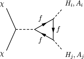
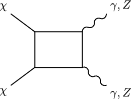
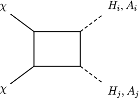
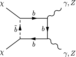
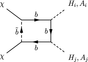
In order to produce a Higgs boson in space and at rest, the DM mass and spin must have specific values. Quantitative statements depend on how many Higgs bosons are produced in the final state. In the case of DM annihilations into two SM-like Higgs bosons, the DM mass must be about 126 GeV (regardless of its spin). If on the contrary, DM annihilations produce only one SM-like Higgs boson plus a photon in the final state, the DM mass must be about GeV (assuming that it has a spin-1/2 or spin-1) while it should be about 109 GeV if it produces a Higgs boson plus a boson in the final state (assuming a spin-0,1/2 or spin-1). In what follows, we will focus on these three specific cases, as they lead to the production of SM-like Higgs bosons at rest but, of course, an analogous analysis can be done for heavier (presumably BSM) Higgs bosons. We now point out some general Higgs boson production mechanisms which could prevail for DM candidates with a mass 63 GeV, 109 GeV and 126 GeV. Examples of relevant Feynman diagrams are given in Fig. 1.



II.1 Production mechanisms for GeV
DM candidates with a mass slightly greater than 126 GeV can produce two Higgs bosons at rest or near rest in the final state either through box diagrams or, if DM is directly coupled to the Higgs, through tree-level process (see Fig. 1).
In a SUSY framework for example, two Higgs bosons can be produced via box diagrams involving, e.g., charginos and boson or quarks and squarks from the third generation [10]. Disregarding for the moment the possible velocity-squared dependence which arises due to the Majorana nature of the neutralino, these diagrams are expected to be relatively suppressed with respect to other annihilation channels which occur at tree-level (such as for example neutralino annihilations into or via a t–channel sbottom or chargino exchange respectively). However they could still be sizable if the Higgs boson has large couplings to the particles in the box or if there is a large mass degeneracy between the neutralino and the chargino () for example (if we consider the box diagram [10, 11, 12, 13]). Alternatively, the DM could also pair annihilate into two Higgs bosons through a pseudo-scalar Higgs boson s–channel exchange. If, in particular, the mass of the pseudo-scalar is about twice the DM mass, one expects a large resonant interaction and potentially a large di-Higgs boson production.
In both cases however, one also expects a large DM pair annihilation rate into two , , , , leading to extra –ray lines. In many scenarios, these process are related, thus giving interesting constraints on the model. However, large branching ratios into , , , , could be detrimental to the searches for a 63 GeV line. For example, in ‘conventional’ BSM scenarios such as SUSY, the di-photon final state is supposed to be slightly larger than the di-Higgs production (notably because it is not phase-space suppressed). Since the di-photon final state relies on charged loop diagrams, one therefore expects a large production of charged particles from the DM pair annihilations at tree-level which poses a problem for the detectability of the 63 GeV line. Indeed, if the contribution from annihilations into -quarks is significant, it is likely that the line at 63 GeV would be totally swamped by the continuum –ray emission resulting from the hadronization, fragmentation and subsequent decay, with an endpoint energy equal to the DM mass, GeV.
There are several ways out, nevertheless. For example, if the charged particles which contribute to the direct photon emission (loop-suppressed) are all heavier than the DM [14], the DM pair annihilation into such particles is not kinematically allowed, thus enabling the di-Higgs final state to be visible. In SUSY, this means that one would have to suppress the t–channel sbottom exchange diagram and perhaps introduce a singlet-like heavy Higgs boson mostly coupled to very heavy charged particles [14]. Alternatively, there could be scenarios where the di-photon and di-Higgs final states are produced by enhanced box diagrams but in which the sbottom exchanges are very suppressed so that the production of -quarks at tree-level is suppressed. In scenarios with a SM-like Higgs boson and no extra pseudo-scalar boson, the tree-level production of -quarks is expected to be velocity-suppressed. If potential loop/box process, susceptible to imply -quarks at tree-level, are also suppressed by the introduction of very heavier mediators, the detectability of the 63 GeV line originating from enhanced box diagrams could be significant.
We also note that in models such as the NMSSM where one can have both a very heavy () and very light () pseudo-scalar Higgs bosons, the requirement of having a resonant exchange if 126 GeV (i.e., GeV) implies that one could also produce at tree-level the final state, with produced at rest. The decay of the into two photons could then generate a line at 126 GeV which could be confused with the direct (resonant) DM pair annihilations into two photons. The dominance of one process over the other would mostly depend on the mass difference and the strength of the coupling of the neutralino to the Higgs boson, which itself is constrained by the width of the invisible Higgs decay channel [15, 16, 17]. Such an ambiguity in the origin of a possible line at GeV in this framework could be of interest in the context of the 130 GeV and 111 GeV bumps observed in the Fermi–LAT data [18, 19, 20, 21, 22, 23, 24, 25].
For candidates with this mass ( 126 GeV), the condition of predicting a 63 GeV line from a SM-like Higgs boson produced at rest guaranties a final state with two SM-like Higgs bosons. However should such a line be seen, one would have to disentangle it from the direct annihilations of DM particles with a mass of GeV into two photons. Also it may be challenging to disentangle the di-Higgs boson final state from the final state. These aspects will be discussed in the next section.
Note that all the final states mentioned above have already been considered in detail in the literature for generic DM masses (see, e.g., Refs. [10, 11, 8]). However, to our knowledge, the –ray signature expected from a Higgs boson decay produced by a GeV DM candidate has not been studied explicitly22 2 –ray fluxes have been calculated and can be obtained from Ref. [26] for different DM masses for DM annihilations into a pair of SM-like Higgs bosons, though.. Many authors have exploited the presence of a single photon in DM pair annihilation final states as a –ray signature [27, 28, 12, 29, 30, 31, 32, 8, 33]. However, the possibility of these prompt photon lines being accompanied by additional lines due to Higgs production at rest has not been pointed out. To our knowledge, the fact that the DM pair annihilation into two photons could be simply confused with a Higgs boson (not necessarily SM-like) production, when , has not been mentioned in the literature yet.
II.2 Production mechanisms for GeV
Due to their mass, candidates with GeV can only produce one SM-like Higgs boson at rest in the final state. The DM spin is then fixed by the nature of the second particle in the final state. The exact final state can also enable one to determine the Higgs boson production mechanism. For example, the final state implies that the Higgs boson production must be a loop-suppressed process since the DM is assumed to be neutral and cannot produce a photon in the final state without coupling to charged particles (unless one considers ‘dipole’ DM [34]).
Usually one exploits the presence of a single photon in the final state to look for such a process (see, e.g., Ref. [8]). However, the corresponding direct –ray line would appear at very low energy, namely GeV, to which Fermi–LAT might still be sensitive. Hence the only line that is experimentally accessible comes from the Higgs decay at 63 GeV. Nevertheless, observing such a line may not unambiguously point towards the production of a Higgs boson: DM pair annihilations into could also produce a monochromatic line at the same energy as the Higgs boson decay if the DM mass is about 63 GeV. Hence, there could be some confusion about the origin of the line, even though such a detection would definitely point towards new physics.
In some models, this possible confusion could be solved by simply comparing the expected cross sections in different channels. For example, in scenarios with photon mixing [35], the s–channel exchange into would be larger than the final state, so a signal at 63 GeV could be expected. However there could be tricky situations. For example, if GeV, both the and process are expected to be very large if they are realized through a Higgs portal, i.e., . The kinematic condition to see a line at GeV indeed immediately implies that the exchange is resonant. Hence, both final states should be copiously produced. If is the SM Higgs boson, the magnitude of versus is fixed by the ratio of the versus the couplings and the phase space factor. Thus, for a SM-like Higgs boson produced very close to rest, the phase space factor eventually suppresses a bit the final state. Yet, ultimately one should detect the sum of the two contributions.
Note that the importance of the and processes through the SM-like Higgs portal ultimately depends on the mass difference , as well as the coupling. The latter can be tuned (in fact reduced) to compensate for the smallness of , in order to avoid too large a resonant annihilation effect, although it cannot be arbitrarily large. The maximum value of the cross section is actually set indirectly by the ATLAS and CMS experiments. The associated cross section is maximal when both becomes smaller than the Higgs boson decay width () and the coupling is maximal. Both are being measured at LHC through the Higgs visible and invisible decay width [36]. A too large coupling would make the Higgs decay invisible and be in conflict with SM predictions.
The above discussion assumes that the DM pair annihilation through the Higgs portal cross section is not velocity-dependent. However, if they turn out to be suppressed and box diagrams are more important, models with kinetic mixing might again lead to a larger value of the cross section for the final state (with respect to the final state).
Would such a line be seen, it would remain to be determined whether it originates from a SM-like Higgs boson decay into two photons or a model of the type discussed above. However, when GeV, the DM pair annihilations into any other channel would produce a –ray spectrum with energies . Hence the line at 63 GeV would not be buried under the continuum spectrum unlike what could occur for GeV, as discussed in the previous subsection.
II.3 Production mechanisms for GeV
When the DM mass is about 109 GeV, the process can occur (for both bosonic and fermionic DM) via a t–channel DM exchange diagram (if DM can couple directly to the Higgs) or a s–channel Z exchange diagram. This process can also occur through box diagrams.
For such a value of the DM mass, both the and SM-like bosons are produced close to rest and should lead to distinctive signatures. In addition to the 63 GeV line from the SM-like Higgs boson decay, there could be a line at 109 GeV coming from the DM annihilations into two photons. Associated with this case, there could also be a line at 72 GeV from the direct photon in the final state if this channel is not suppressed. The dominance of one over the other one depends again on the couplings and exact process, while their visibility essentially depends on the background at these energies. Note that –ray line at 109 GeV from direct annihilation into two photons could be consistent with the possible line detected at 111 GeV [20, 21] and could be used to constrain the DM interactions.
II.4 Additional remarks
The results displayed in the next section hold independently of whether the new particle discovered at CERN is the Higgs boson or not. Since the observed branching ratios are compatible with the SM Higgs predictions (within 2 ), our conclusion regarding whether one can see a monochromatic line at GeV should remain identical.
Some of the Higgs production mechanisms that we discuss in this paper may be associated with a large spin-independent elastic scattering cross section with a nucleon and could be ruled out by DM direct detection experiments. In particular if the DM has a mass in the GeV-TeV range, its interactions could be severely constrained by the XENON100 experiment [37, 38]. Since this requires to specify a model and we intend to set model-independent constraints, we assume that the underlying DM particle model is compatible with the results from the latest direct detection experiments. However, for concrete models such a compatibility has to be checked.
II.5 Detectability of the line emission and continuum

The –ray emission subsequent to Higgs production typically occurs from the Higgs boson decay into, e.g., , , etc. Since all the channels have very well-known branching ratios, the –ray flux can be predicted quite accurately (albeit astrophysical uncertainties).
Predictions depend on the photon energy spectrum associated with the Higgs boson decay. Typically, for a Higgs boson of about 126 GeV produced at rest, one expects a smooth spectrum (due to dominant decay into ) plus a monochromatic line due to [39, 40, 41]. In the SM, (for GeV) the Higgs boson decay into is suppressed by a factor of with respect to the final state [41], so one may think that the –ray line is hidden by the continuum. However, channels such as emit photons at lower energies than (owing to final state radiation, hadronization, fragmentation and decay). As a result, even though the flux associated with the monochromatic line is meant to be suppressed, in principle it could be distinguishable from the continuum emission. In order to compute the spectrum, we use PYTHIA 6.4 [42], where we set the branching ratio for to [41] 33 3 Note that the default value in PYTHIA 6.4 is . Also notice that the best fit for the LHC measurement is 2.9 times the SM value and, at 95% confidence level, it could be up to 5.4 times the SM one [46] (see also Refs. [47, 48, 49, 50]).. The result is displayed in Fig. 2. Clearly, the monochromatic line appears to be distinguishable from the smooth spectrum, even though it is suppressed.
Now, we estimate the associated flux from DM annihilations (an analogous analysis could be performed for decaying DM) around the galactic center and compare it to the current Fermi–LAT data. We will assume a generic DM candidate, with a thermal average of the annihilation cross section times the relative velocity of , where in each case we consider that the only annihilation channel is , or .
The differential flux of prompt –rays generated from DM annihilations in the smooth DM halo from a direction within a solid angle is given by [28]
| (1) |
where is the differential –ray yield, is a symmetry factor which for Majorana DM is equal to 1 and 1/2 if DM is not a self-conjugate particle, is the DM density profile and is the distance from the galactic center. The spatial integration of the square of the DM density profile is performed along the line of sight within the solid angle of observation . More precisely, , and the upper limit of integration is , where is the angle between the direction of the galactic center and that of observation and is the distance from the Sun to the galactic center. Being the contributions at large scales negligible, the choice of the size of the Milky Way halo, is not crucial.
Thus, the flux of DM annihilations can be written as
| (2) |
with the dimensionless quantity defined as
| (3) |
where for the distance from the Sun to the galactic center and for the local DM density we use kpc and GeV/cm3, respectively [43].

Although for some DM density profiles, the integration of in the solid angle of observation can be done analytically [44], here we consider an Einasto profile [45], for which there is no analytical solution, and compute it numerically. This density profile is parametrized as
| (4) |
where kpc is a characteristic length.
Following Refs. [51, 52, 53, 54, 55], we consider a squared region centred on the galactic center, for which . In Fig. 3 we compare the expected flux from this region and compare it with the Fermi–LAT data. To obtain the measured flux, we take the Fermi–LAT data obtained from August 4, 2008 to October 1, 2012. We extract the data from the Fermi Science Support Center archive [56] and select only events classified as CLEAN. We use a zenith angle cut of 105∘ to avoid contamination by the Earth’s albedo and the instrument response function P7CLEAN_V6.
In the upper panel of Fig. 3 we show the –ray spectra for three different annihilation channels, (upper red line), (black dotted line) and (orange line), in which the Higgs is produced very close to rest. The DM mass for each case is GeV, GeV and GeV, respectively. As can be seen from the plot, the fluxes for the three cases are very similar, but the final state is slightly more visible than the two others44 4 Let us stress again that the –rays in this case are only those coming from Higgs decay. For GeV, the direct photon lies at energies well below detection threshold for Fermi–LAT., mainly because of the lower value of the DM mass in this case. Since the flux scales linearly with the cross section, these lines emerge from the –ray background when the associated production cross section is greater than for (), thereby ruling out a Higgs boson production cross section larger than this value. This can be seen from the lower panel of Fig. 3, where we show the value of for which the signal would be equal to the observed background. Interestingly enough, for the case of DM annihilations into or , producing Higgs at rest, the –ray line from the very suppressed channel (see Fig. 2), is expected to provide a more restrictive limit than the dominant continuum.
The limits that we sketch are very conservative as they assume no background from astrophysical sources. A dedicated search for Higgs boson decay lines would require to account for the background modeling and to optimize the detection window [18, 19, 20, 21, 22, 23, 24, 25]. However here we simply want to illustrate the potential detectability of these lines. Note that our limits are in agreement with the detailed Fermi–LAT searches of –ray lines [57]. These were obtained by the Fermi–LAT analysis for GeV and can be directly compared to the ones presented here for and GeV. While the Fermi–LAT limit is (cf. Fig. 15 in Ref. [57]), we obtain , the difference coming from the branching ratio for . Similarly, for the case of and GeV, the limit obtained from the -ray line from Higgs decay is just a factor of 2 weaker than that for and GeV (explained as a factor of 2 in favour of due to having two Higgs bosons and a factor of 4 in favour of due to the factor of two in the DM mass).
In DM models where there is a correlation between the di-photon and , and/or final states, the ratio of the flux associated with the prompt -ray line to that of the Higgs boson decay line can be used to test the model. In particular when GeV, one expects the following ratio .
In the absence of evidence for a specific DM model and a precise correlation between these two final states, searching for the Higgs decay line could allow us to obtain a constraint on the DM-Higgs boson interactions. The main difficulty associated with these searches consists in removing the astrophysical background sources but these searches are worthwhile, as they could reveal new physics and point towards models with multiple scalar and pseudo-scalar Higgs bosons with large DM-Higgs couplings, for example.
III Boosted Higgs and multiple Higgs bosons scenarios
We can now investigate the case of boosted Higgs production and multiple Higgs scenarios.
III.1 Boosted Higgs boson
The Higgs boson decay line considered in the previous section is now replaced by a broad excess which shows up as a less prominent feature. For , this box-shaped part of the spectrum is a particular case of those studied in Ref. [58]. However, in the cases discussed here, this broad excess is accompanied by a smooth spectrum from the Higgs decay into all other possible channels plus a possible line due to prompt photon emission in the final state.
These features are illustrated in Fig. 4, where the –ray spectrum due to Higgs decay for a Higgs boson ( GeV) produced with an energy GeV is depicted. Over the continuum from the other Higgs decay channels, a bump at 60 GeV, corresponding to the Higgs boson decay into two photons, can still be distinguished. Below 10 GeV, the continuum is two orders of magnitude (or more) brighter than the line, so the limit on the Higgs boson production, for DM masses for which the Higgs boson is boosted, is actually obtained from the continuum rather than from the broad excess at 60 GeV. This can be seen in Fig. 5, which is analogous to Fig. 3, but now for GeV (), 111 GeV () and 130 GeV (), such that, for all these cases, the produced Higgs has an energy close to 130 GeV.

For the final state, note that there is a –ray line emitted at 32 GeV, in addition to the box-shaped spectrum at 50–80 GeV and the continuum from Higgs decays. This line originates from the prompt in the final state and provides the most stringent bound on Higgs boson production cross section. Actually, in the case of , the prompt –ray is always in the energy window accessible by Fermi–LAT if the Higgs is not produced very close to rest. Using the Fermi–LAT data for this annihilation channel and for GeV, we obtain a limit of about . This is comparable to the –ray line limits obtained by Fermi–LAT for with GeV, that is (cf. Fig. 15 in Ref. [57]), after correcting the cross section limit by a factor of to account for the fact that there is only one prompt photon in the final state with respect to and that the DM mass is different.

III.2 Multiple Higgs bosons scenarios
In minimal SUSY models, in addition to a SM-like Higgs, one expects a heavier CP-even Higgs () and a heavier CP-odd Higgs (A). If the heavier CP-odd Higgs boson mass is about , annihilations into through CP-odd Higgs portal could be resonant and produce a line at . In fact, this process has been proposed to explain the bump at 130 GeV in the Fermi–LAT data [59, 60, 61]. In these configurations, the and final states might be possible too, leading to the production of a CP-odd Higgs boson on-shell or slightly boosted CP-even if . These final states should be slightly suppressed with respect to the final states due to the phase-space suppression factor, but would still contribute to the –ray data at .
In the NMSSM, final states such as and may be possible too, with a second pseudo-scalar Higgs boson which can be light and two heavy Higgs bosons [62]. Such final states could lead to the production of Higgs bosons produced at rest when and could be resonant when . The same process could be in fact relevant for low DM mass scenarios such as those discussed in Ref. [7].
IV Conclusions
In this Letter, we have considered the –ray signatures from the decay of a Higgs boson produced in our galactic halo from DM annihilations. We have considered, in particular, the case where the Higgs boson is SM-like (with a mass of 126 GeV and SM branching ratios) and showed that the Higgs boson production cross section for annihilating DM particles with masses 63 GeV, 109 GeV and 126 GeV (Higgs produced very close to rest), cannot exceed . The limit is in fact mostly driven by the –ray line from . These results can be trivially generalised to other Higgs boson masses (as relevant in BSM models with multiple Higgs bosons and Higgs mass spectrum such as the NMSSM) leading to different DM scenarios.
We have also considered the case of a slightly boosted Higgs boson and shown that the associated signature would exhibit a broad (box-shaped) –ray excess. However, the continuum associated with the other Higgs boson decay modes and to the second particle in the final state would lead to a brighter –ray emission, which can be used to constrain the Higgs boson production cross section. Focusing in particular on the final state for a SM-like Higgs boson produced with an energy GeV, we find that the Higgs boson production cross section cannot exceed .
Therefore, we have obtained a simple estimate for the limit on the Higgs boson production cross section that is independent of any other DM annihilation channels and demonstrates that performing Higgs boson decay line searches could be useful to probe the Higgs boson dark couplings (i.e., couplings to DM particles). This must be compared to the limits set on the invisible Higgs boson decay branching ratios obtained by using LHC measurements (cf., for example, Ref. [17]), but the two approaches (collider and indirect detection searches) are complementary.
Acknowledgments
We would like to thank M. Cirelli, M. Dolan, G. Gómez-Vargas and C. McCabe for useful discussions. NB is supported by the DFG TRR33 ‘The Dark Universe’. CB and SPR thank the Galileo Galilei Institute for Theoretical Physics for its hospitality. JS and CB are supported by the ERC advanced grant ‘DARK’ at IAP, Paris. SPR is partially supported by the Portuguese FCT through CERN/FP/123580/2011 and CFTP-FCT UNIT 777, which are partially funded through POCTI (FEDER) and by the Spanish Grant FPA2011-23596 of the MINECO. TT is supported by the European ITN project (FP7-PEOPLE-2011-ITN, PITN-GA-2011-289442-INVISIBLES). Numerical computation in this work was partially carried out at the Yukawa Institute Computer Facility.
References
- [1] S. Chatrchyan et al. (CMS Collaboration), Phys.Lett. B710, 403 (2012a), eprint 1202.1487.
- [2] S. Chatrchyan et al. (CMS Collaboration), Phys.Lett. B710, 26 (2012b), eprint 1202.1488.
- [3] G. Aad et al. (ATLAS Collaboration), Phys.Rev.Lett. 108, 111803 (2012a), eprint 1202.1414.
- [4] G. Aad et al. (ATLAS Collaboration), Phys.Lett. B710, 49 (2012b), eprint 1202.1408.
- [5] A. Arbey, M. Battaglia, A. Djouadi, and F. Mahmoudi, JHEP 1209, 107 (2012), eprint 1207.1348.
- [6] C. Englert, J. Jaeckel, E. Re, and M. Spannowsky, Phys.Rev. D85, 035008 (2012a), eprint 1111.1719.
- [7] D. A. Vásquez, G. Bélanger, C. Boehm, J. Da Silva, P. Richardson, and C. Wymant, Phys.Rev. D86, 035023 (2012), eprint 1203.3446.
- [8] C. Jackson, G. Servant, G. Shaughnessy, T. M. Tait, and M. Taoso, JCAP 1004, 004 (2010), eprint 0912.0004.
- [9] R. Laha, K. C. Y. Ng, B. Dasgupta, and S. Horiuchi, Phys.Rev. D87, 043516 (2013), eprint 1208.5488.
- [10] L. Bergström and P. Ullio, Nucl.Phys. B504, 27 (1997), eprint hep-ph/9706232.
- [11] Z. Bern, P. Gondolo, and M. Perelstein, Phys.Lett. B411, 86 (1997), eprint hep-ph/9706538.
- [12] F. Boudjema, A. Semenov, and D. Temes, Phys.Rev. D72, 055024 (2005), eprint hep-ph/0507127.
- [13] G. Bélanger, C. Boehm, M. Cirelli, J. Da Silva, and A. Pukhov, JCAP 1211, 028 (2012), eprint 1208.5009.
- [14] M. Dolan and C. McCabe, Article in preparation.
- [15] R. E. Shrock and M. Suzuki, Phys.Lett. B110, 250 (1982).
- [16] M. Pospelov and A. Ritz, Phys.Rev. D84, 113001 (2011), eprint 1109.4872.
- [17] C. Englert, M. Spannowsky, and C. Wymant, Phys.Lett. B718, 538 (2012b), eprint 1209.0494.
- [18] T. Bringmann, X. Huang, A. Ibarra, S. Vogl, and C. Weniger, JCAP 1207, 054 (2012), eprint 1203.1312.
- [19] C. Weniger, JCAP 1208, 007 (2012), eprint 1204.2797.
- [20] A. Rajaraman, T. M. Tait, and D. Whiteson, JCAP 1209, 003 (2012), eprint 1205.4723.
- [21] M. Su and D. P. Finkbeiner (2012a), eprint 1206.1616.
- [22] M. Su and D. P. Finkbeiner (2012b), eprint 1207.7060.
- [23] T. Bringmann and C. Weniger, Phys.Dark Univ. 1, 194 (2012), eprint 1208.5481.
- [24] A. Hektor, M. Raidal, and E. Tempel (2012), eprint 1209.4548.
- [25] D. P. Finkbeiner, M. Su, and C. Weniger, JCAP 1301, 029 (2013), eprint 1209.4562.
- [26] M. Cirelli, G. Corcella, A. Hektor, G. Hutsi, M. Kadastik, et al., JCAP 1103, 051 (2011), eprint 1012.4515.
- [27] P. Ullio and L. Bergström, Phys.Rev. D57, 1962 (1998), eprint hep-ph/9707333.
- [28] L. Bergström, P. Ullio, and J. H. Buckley, Astropart.Phys. 9, 137 (1998), eprint astro-ph/9712318.
- [29] M. Perelstein and A. Spray, Phys.Rev. D75, 083519 (2007), eprint hep-ph/0610357.
- [30] M. Gustafsson, E. Lundstrom, L. Bergström, and J. Edsjö, Phys.Rev.Lett. 99, 041301 (2007), eprint astro-ph/0703512.
- [31] E. Dudas, Y. Mambrini, S. Pokorski, and A. Romagnoni, JHEP 0908, 014 (2009), eprint 0904.1745.
- [32] Y. Mambrini, JCAP 0912, 005 (2009), eprint 0907.2918.
- [33] G. Bertone, C. Jackson, G. Shaughnessy, T. M. Tait, and A. Vallinotto, JCAP 1203, 020 (2012), eprint 1009.5107.
- [34] K. Sigurdson, M. Doran, A. Kurylov, R. R. Caldwell, and M. Kamionkowski, Phys.Rev. D70, 083501 (2004), eprint astro-ph/0406355.
- [35] H. Davoudiasl, H.-S. Lee, and W. J. Marciano, Phys.Rev. D85, 115019 (2012), eprint 1203.2947.
- [36] B. A. Dobrescu and J. D. Lykken, JHEP 1302, 073 (2013), eprint 1210.3342.
- [37] E. Aprile et al. (XENON100 Collaboration), Phys.Rev.Lett. 109, 181301 (2012), eprint 1207.5988.
- [38] J. H. Davis, T. Ensslin, and C. Boehm (2012), eprint 1208.1850.
- [39] J. R. Ellis, M. K. Gaillard, and D. V. Nanopoulos, Nucl.Phys. B106, 292 (1976).
- [40] A. Djouadi, M. Spira, and P. Zerwas, Phys.Lett. B311, 255 (1993), eprint hep-ph/9305335.
- [41] S. Dittmaier et al. (2012), eprint 1201.3084.
- [42] T. Sjöstrand, S. Mrenna, and P. Z. Skands, JHEP 0605, 026 (2006), eprint hep-ph/0603175.
- [43] R. Catena and P. Ullio, JCAP 1008, 004 (2010), eprint 0907.0018.
- [44] J. Lavalle, C. Boehm, and J. Barthes, JCAP 1002, 005 (2010), eprint 0907.5589.
- [45] J. Einasto, Trudy Inst. Astrofiz. Alma-Ata 51, 87 (1965).
- [46] T. Corbett, O. Éboli, J. González-Fraile, and M. González-García, Phys.Rev. D86, 075013 (2012), eprint 1207.1344.
- [47] D. Carmi, A. Falkowski, E. Kuflik, and T. Volansky, JHEP 1207, 136 (2012), eprint 1202.3144.
- [48] A. Azatov, R. Contino, and J. Galloway, JHEP 1204, 127 (2012), eprint 1202.3415.
- [49] J. Espinosa, C. Grojean, M. Mühlleitner, and M. Trott, JHEP 1205, 097 (2012), eprint 1202.3697.
- [50] M. Montull and F. Riva, JHEP 1211, 018 (2012), eprint 1207.1716.
- [51] P. D. Serpico and G. Zaharijas, Astropart. Phys. 29, 380 (2008), eprint 0802.3245.
- [52] T. E. Jeltema and S. Profumo, JCAP 0811, 003 (2008), eprint 0808.2641.
- [53] L. Pieri, J. Lavalle, G. Bertone, and E. Branchini, Phys. Rev. D83, 023518 (2011), eprint 0908.0195.
- [54] N. Bernal and S. Palomares-Ruiz, Nucl.Phys. B857, 380 (2012a), eprint 1006.0477.
- [55] N. Bernal and S. Palomares-Ruiz, JCAP 1201, 006 (2012b), eprint 1103.2377.
- [56] http://fermi.gsfc.nasa.gov/cgi-bin/ssc/LAT/LATDataQuery.cgi.
- [57] M. Ackermann et al. (Fermi-LAT Collaboration), Phys.Rev. D86, 022002 (2012), eprint 1205.2739.
- [58] A. Ibarra, S. López Gehler, and M. Pato, JCAP 1207, 043 (2012), eprint 1205.0007.
- [59] L. López-Honorez, T. Schwetz, and J. Zupan, Phys.Lett. B716, 179 (2012), eprint 1203.2064.
- [60] D. Das, U. Ellwanger, and P. Mitropoulos, JCAP 1208, 003 (2012), eprint 1206.2639.
- [61] L. Wang and X.-F. Han, Phys.Rev. D87, 015015 (2013), eprint 1209.0376.
- [62] J. F. Gunion, Y. Jiang, and S. Kraml, Phys.Rev. D86, 071702 (2012), eprint 1207.1545.