Teichmüller Extremal Mapping and its Applications to Landmark Matching Registration
Abstract
Registration, which aims to find an optimal 1-1 correspondence between shapes, is an important process in different research areas. Conformal mappings have been widely used to obtain a diffeomorphism between shapes that minimizes angular distortion. Conformal registrations are beneficial since it preserves the local geometry well. However, when landmark constraints are enforced, conformal mappings generally do not exist. This motivates us to look for a unique landmark matching quasi-conformal registration, which minimizes the conformality distortion. Under suitable condition on the landmark constraints, a unique diffeomporphism, called the Teichmüller extremal mapping between two surfaces can be obtained, which minimizes the maximal conformality distortion. In this paper, we propose an efficient iterative algorithm, called the Quasi-conformal (QC) iterations, to compute the Teichmüller mapping. The basic idea is to represent the set of diffeomorphisms using Beltrami coefficients (BCs), and look for an optimal BC associated to the desired Teichmüller mapping. The associated diffeomorphism can be efficiently reconstructed from the optimal BC using the Linear Beltrami Solver(LBS). Using BCs to represent diffeomorphisms guarantees the diffeomorphic property of the registration. Using our proposed method, the Teichmüller mapping can be accurately and efficiently computed within 10 seconds. The obtained registration is guaranteed to be bijective. The proposed algorithm can also be extended to compute Teichmüller mapping with soft landmark constraints. We applied the proposed algorithm to real applications, such as brain landmark matching registration, constrained texture mapping and human face registration. Experimental results shows that our method is both effective and efficient in computing a non-overlap landmark matching registration with least amount of conformality distortion.
keywords
Teichmüller extremal mapping, quasi-conformal mapping, Beltrami coefficient, Linear Beltrami Solver, Landmark matching registration1 Introduction
Registration refers to the process of finding an optimal one-to-one correspondence between images or surfaces. It has been extensively applied to different areas such as medical imaging, computer graphics and computer visions. For example, in medical imaging, registration is always needed for statistical shape analysis, morphometry and processing of signals on brain surfaces (e.g., denoising or filtering). While in computer graphics, surface registration is needed for texture mapping, which align each vertex to a position of the texture image, to improve the visualization of the surface mesh. Developing an effective algorithm for registration is therefore very important.
Conformal mappings have been widely used to obtain smooth 1-1 correspondences between different domains that minimize angular distortions. Conformal mappings are advantageous since it preserves the local geometry well. According to the conformal geometry, given two simply-connected domains, there always exists a unique conformal mapping between them up to a Mobiüs transformation. However, the existence of conformal mappings cannot be guaranteed in general situations. For example, conformal mapping between two multiply-connected domains usually does not exist. Besides, in practical situation, obtaining a registration that matches landmark features consistently are often required. When landmark constraints are enforced, the existence of conformal mappings cannot be guaranteed. This motivates us to look for a unique landmark-matching registration, which minimizes the conformality distortion as much as possible.
Under suitable conditions on the landmark constraints, there exists a unique quasi-conformal mapping, called the Teichmüller extremal mapping, which minimizes the maximal conformality distortion. To compute this Teichmüller mapping, we propose in this paper an efficient and effective iterative algorithm, which is called the Quasi-conformal (QC) iterations. The basic idea is to represent the set of diffeomorphisms using Beltrami coefficients (BCs), and look for an optimal BC associated to the desired Teichmüller mapping. The associated diffeomorphism can be efficiently reconstructed from the optimal BC using the Linear Beltrami Solver(LBS). Given a set of landmark constraints, the algorithm is able to determine an optimal 1-1 correspondence (including the boundary correspondence in the case of open surfaces) between shapes automatically, which minimizes the conformality distortion. Besides, the proposed algorithm can also compute extremal mapping with soft landmark constraints. It becomes necessary when landmark features cannot be accurately located, and hence it is better to compute registration with landmarks approximately (but not exactly) matched. Another major advantage of using Teichmüller mappings for landmark matching registrations is that the bijectity (1-1, onto) of the registrations can be guaranteed. Obtaining a bijective landmark matching registration is generally difficult, especially when a large number of landmark constraints are enforced. Using our proposed method, a bijective Teichmüller mapping can be accurately and efficiently computed within 10 seconds. To test the effectiveness of our method, we applied the proposed algorithm to real applications, such as brain registration, constrained texture mapping and human face registration. Experimental results shows that our method is both effective and efficient in computing a non-overlap landmark matching registration with least conformality distortion.
In short, the contributions of this paper are three-folded. Firstly, we propose an efficient algorithm for obtaining the unique Teichmüller extremal mapping between shapes with landmark constraints enforced. The mapping is guaranteed to be bijective and minimizes the maximal conformality distortion. Secondly, we propose an algorithm to compute Teichmüller extremal mapping with soft landmark constraints. Landmarks are not exactly matched, but less conformality distortion will be introduced. Thirdly, we apply the proposed algorithms to real applications, namely, constrained texture mapping, medical image registration and human face registration.
2 Previous work
In this section, we will introduce some previous works closely related to our paper.
Surface parameterization and registration have been extensively studied, for which different kinds of bijective surface maps have been proposed. Conformal registration, which minimizes angular distortion, have been widely used to obtain a smooth 1-1 correspondence between surfaces [6, 7, 9, 3, 11, 8]. For example, Hurdal et al. [11] proposed to compute the conformal parameterizations using circle packing and applied it to registration of human brains. Gu et al. [7, 9, 8] proposed to compute the conformal parameterizations of Riemann surfaces for registration using harmonic energy minimization and holomorphic 1-forms. Later, the authors proposed the curvature flow method to compute conformal parameterizations of high-genus surfaces onto their universal covering spaces [32, 33, 34]. Conformal registration is advantageous for it preserves the local geometry well.
Sometimes, deformations between objects might not not conformal. Instead, certain amount of angular distortion could be introduced. To tackle with this situation, quasi-conformal mappings are proposed to obtain smooth 1-1 correspondence with bounded conformality distortion. Lui et al. [18] proposes to compute quasi-conformal registration between hippocampal surfaces which matches geometric quantities (such as curvatures) as much as possible. A method called the Beltrami Holomorphic flow is used to obtain the optimal Beltrami coefficient associated to the registration [17]. Beltrami coefficient has been applied to represent general surface homeomorphisms, which is comparatively easier to manipulate than 3D coordinate functions. Using Beltrami representation, compression of surface maps has been proposed [16], which can be applied for video compression [20]. Wei et al. [31] also proposes to compute quasi-conformal mapping for feature matching face registration. The Beltrami coefficient associated to a landmark points matching parameterization is approximated. However, either exact landmark matching or the bijectivity of the mapping cannot be guaranteed, especially when very large deformations occur. In order to compute quasi-conformal mapping from the Beltrami coefficients effectively. Quasi-Yamabe method is introduced, which applies the curvature flow method to compute the quasi-conformal mapping [19]. The algorithm can deal with surfaces with general topologies. Later, quasi-conformal mapping, which minimizes the conformality distortion, has been studied. Zorin et al. [36] proposes an algorithm to compute the extremal quasi-conformal mapping between connected domains with given Dirichlet condition defined on the whole boundaries. The extremal mapping is obtained by minimizing a least square Beltrami energy, which is non-convex. The algorithm can obtain an extremal mapping when initialization is carefully chosen. However, the convergence to the global minimum cannot be guaranteed.
Most of the above registration algorithms using conformal and quasi-conformal mappings cannot match feature landmarks, such as sulcal landmarks on the human brains, consistently. To alleviate this issue, landmark-matching registration algorithms are proposed by various research groups. Wang et al. [12, 15, 13, 14, 10, 35] proposed to compute the optimized conformal parameterizations of brain surfaces by minimizing a compounded energy [12, 15]. The obtained registration can obtain an optimized conformal map that better aligns the features, however, landmarks cannot be exactly matched. Besides, bijectivity cannot be ensured when large number of landmark constraints are enforced. To solve this problem, smooth vector field has also been applied to obtain surface registration. Lui et al. [13, 14] proposed the use of vector fields to represent surface maps and reconstruct them through integral flow equations. They obtained shape-based landmark matching harmonic maps by looking for the best vector fields minimizing a shape energy. The use of vector fields to compute the registration makes optimization easier, although it cannot describe all surface maps. An advantage of this method is that exact landmark matching can be guaranteed. Time dependent vector fields can also be used. For example, Joshi et al. [10] proposed the generation of large deformation diffeomorphisms for landmark point matching, where the registrations are generated as solutions to the transport equation of time dependent vector fields. The time dependent vector fields facilitate the optimization procedure, although it may not be a good representation of surface maps since it requires more memory. The computational cost of the algorithm is also expensive.

3 Mathematical Background
In this section, we describe some basic mathematical concepts related to our algorithms. For details, we refer the readers to [5, 21, 22].
A surface with a conformal structure is called a Riemann surface. Given two Riemann surfaces and , a map is conformal if it preserves the surface metric up to a multiplicative factor called the conformal factor. An immediate consequence is that every conformal map preserves angles. With the angle-preserving property, a conformal map effectively preserves the local geometry of the surface structure.
A generalization of conformal maps is the quasi-conformal maps, which are orientation preserving homeomorphisms between Riemann surfaces with bounded conformality distortion, in the sense that their first order approximations takes small circles to small ellipses of bounded eccentricity [5]. Mathematically, is quasi-conformal provided that it satisfies the Beltrami equation:
| (1) |
for some complex valued function satisfying . is called the Beltrami coefficient, which is a measure of non-conformality. In particular, the map is conformal around a small neighborhood of when . Infinitesimally, around a point , may be expressed with respect to its local parameter as follows:
| (2) |
Obviously, is not conformal if and only if . Inside the local parameter domain, may be considered as a map composed of a translation to together with a stretch map , which is postcomposed by a multiplication of which is conformal. All the conformal distortion of is caused by . is the map that causes to map a small circle to a small ellipse. From , we can determine the angles of the directions of maximal magnification and shrinking and the amount of them as well. Specifically, the angle of maximal magnification is with magnifying factor ; The angle of maximal shrinking is the orthogonal angle with shrinking factor . Thus, the Beltrami coefficient gives us all the information about the properties of the map (See Figure 4(D)).


The maximal dilation of is given by:
| (3) |
Let . From the Beltrami equation (1),
| (4) |
Let . We can write and as linear combinations of and ,
| (5) |
where ; ; .
Similarly,
| (6) |
Since , we obtain
| (7) |
Quasiconformal mapping between two Riemann surfaces and can also be defined. Instead of the Beltrami coefficient, the Beltrami differential has to be used. A Beltrami differential on the Riemann surface is an assignment to each chart of an complex-valued function , defined on local parameter such that
| (8) |
on the domain which is also covered by another chart , where and (See Figure 2).
An orientation preserving diffeomorphism is called quasi-conformal associated with if for any chart on and any chart on , the mapping is quasi-conformal associated with (See Figure 3.
Now, suppose and are open Riemann surfaces with the same topology. The boundary dilation of is the infimum of the maximal dilation of over all quasi-conformal maps isotopic to relative to the boundary and all neighborhoods of .
In case and are simply-connected, conformal mapping between and always exists. However, conformal mapping may not exist between multiply-connected domains. For example, there is generally no conformal mapping between two annuli with different radii of inner circles. One might be interested in investigating extremal quasiconformal mappings, which is extremal in the sense of minimizing the over all Beltrami differentials corresponding to quasi-conformal mappings between and . Extremal mapping always exists but need not be unique. More specifically, an extremal quasi-conformal mapping can be defined mathematically as follows:
3.1.
Let be a quasi-conformal mapping between and . is said to be an extremal mapping if for any quasi-conformal mapping isotopic to relative to the boundary,
| (9) |
It is uniquely extremal if the inequality (9) is strict.
Another kind of mapping, called the Teichmüller mapping, is closely related to extremal mapping. Teichmüller mapping is defined as follows:
3.2.
Let be a quasi-conformal mapping. is said to be a Teichmüller mapping associated with if its associated Beltrami coefficient is of the form:
| (10) |
for some constant and .

Extremal mapping is not unique for general cases. However, a Teichmüller mapping associated with a holomorphic function is the unique extremal mapping in its homotopic class. The Strebel’s theorem explains the relationship bewtween Teichmüller mapping and extremal mapping.
3.3 (Strebel’s theorem).
Let be an extremal quasi-conformal mapping with . If , then is a Teichmuller map associated with an integrable holomorphic quadratic function on . Hence, is also an unique extremal mapping.
In particular, Teichmüller mapping and extremal mapping of the unit disk are closely related.
3.4.
Let be an orientation-preserving homeomorphism of . Suppose further that and is bounded. Then there is a Teichmüller mapping of finite norm that is the uniquely extremal extension of to . That is, is an extremal mapping with .
In other words, an extremal mapping of the unit disk with suitable boundary condition is a Teichmüller mapping. It can thus be obtained by searching for an optimal Beltrami coefficient whose maximal dilatation is the minimum, while its norm is constant everywhere. It turns out that in most situations, extremal quasi-conformal mapping is a Teichmüller mapping (even for domains with non-trivial topologies). In some rare situations when an extremal mapping is not exactly a Teichmüller mapping, one can get a Teichmüller mapping whose dilation is arbitrarily close to the extremal dilation.
3.5.
Let be a class of quasi-conformal mappings between the open Riemann surfaces and , which are homotopic modulo the boundary. Let be the smallest maximal dilation of the mappings in . Then there are Teichmüller mappings in , associated with a meromorphic function with at most one simple pole, whose dilation is arbitrarily close to .
4 Mathematical Formulation
In this section, we give the mathematical formulation for obtaining the Teichmüller extremal mapping with least conformality distortion. We propose to use the Beltrami coefficient(BC) to represent the mapping, instead of the commonly used representations by deformation fields or coordinate functions. The diffeomorphic property of the registration can then be effectively controlled. Our goal is to formulate the problem into a variational problem to obtain an optimal BC, , associated to the desired extremal mapping .
Suppose and are two domains in the complex plane with the same topology. and can either be simply-connected or multiply-connected. Suppose the boundary condition of the desired extremal mapping is known. Denote it by . The Teichmüller extremal mapping can be mathematically described as follows:
| (11) |
for some constant and holomorphic function .
Recall that a Teichmüller extremal mapping is extremal in the sense of minimizing the over all Beltrami differentials corresponding to quasiconformal mappings in the Teichmüller equaivalence class. In other words, for any satisfying , we have
| (12) |
where and are the Beltrami coefficient of and respectively. Hence, our original problem (11) can be formulated as a variational problem as follows:
| (13) |
subject to:
- •
(boundary condition);
- •
for some constant and holomorphic function .
Theoretically, a diffeomorphism is associated to a unique smooth BC with . The Beltrami coefficient measures the conformality distortion of the map . It can be considered as a unique representation of . The first term of the energy functional aims to minimize the maximal conformality distortion of the mapping. The second term minimizes the harmonic energy of . Since a Teichmüller map has a constant norm, minimizing the second term aims to obtain a optimal BC whose norm is constant.
However, minimizing with respect to the space of diffeomorphisms between and is difficult.
| (14) |
subject to and for some constant and holomorphic function .
In order to minimize the above constrained minimization effectively, we propose to reformulate the energy functional with respect to space of all Beltrami coefficients:
| (15) |
subject to:
- •
and ;
- •
for some constant and holomorphic function ;
- •
(boundary condition).
In other words, the minimization problem (13) is reformulated to be optimized with respect to BCs, which are complex-valued functions defined on . Minimizing the energy functional with respect to BCs is advantageous since the diffeomorphic property of the mapping can be easily controlled. Every diffeomorphism is associated to a smooth Beltrami coefficient . measures the bijectivity (1-1 and onto) of . In fact, is related to the Jacobian of by the following formula:
| (16) |
Therefore, the map is bijective if is everywhere less than 1. When solving the minimization problem (15), the bijectivity of the mapping in each iterations can be ensured by enforcing . Our goal is to look for an optimized smooth BC, , such that its associated quasi-conformal map is our desired Teichmüller extremal mapping.
The boundary condition in the variational problem (15) can be relaxed. The Dirichlet condition defined on the whole boundary is not required. Also, interior landmark constraints can be enforced. Our goal is to solve the variational problem with these landmark constraints, which determine the optimal 1-1 correspondence (including the boundary correspondence) automatically. In other words, the boundary condition in the problem (15) can be reformulated as:
| (17) |
where and are corresponding landmark points or curves defined on and respectively; and and are corresponding interior landmark points of curves in and respectively. By optimizing the energy functional 15, an optimized Teichmüller extremal mapping can be obtained, which matches landmark features consistently while minimizing the maximal conformality distortion.
Note also that the above formulation is designed for extremal mapping of 2D connected domains. However, it can easily be extended to simply-connected or multiply-connected open surfaces. Let and be two connected open surfaces with the same topology. We can conformally parameterize and by and respectively. Then the extremal mapping between and induces an extremal mapping . All the above formulation applies to . In other words, the computation of the extremal mapping between connected surfaces embedded in can be reduced to the computation of the extremal mapping between the conformal domains in .
In the subsequent section, we propose an algorithm, called the quasi-conformal (QC) iteration to solve the above minimization problems (15).
5 Main Algorithm
In this section, we describe an iterative scheme, called the quasi-conformal (QC) iteration, for solving the variational problem (15). The QC iteration is based on the Linear Beltrami Solver(LBS). The LBS will firstly be explained in detail. QC iteration will then be described.
Practically speaking, 2D domains or surfaces in are usually represented discretely by triangular meshes. Suppose and are two surface meshes with the same topology representing and . We define the set of vertices on and by and respectively. Similarly, we define the set of triangular faces on and by and . Our goal is to look for a piecewise linear homeomorphism between and that approximates the Teichmüller extremal mapping between and .
5.1 Linear Beltrami Solver
Our goal is to look for an optimal Beltrami coefficient(BC) associated to the desired Teichmüller mapping. Every quasi-conformal mapping is associated to a unique BC. Given a BC, it is important to have an algorithm to reconstruct the associated quasi-conformal homeomorphism.
Suppose is an orientation preserving piecewise linear homeomorphism between and . We can assume and are both embedded in . In case and are surface meshes in , we first parameterize them conformally by and . The composition of with the conformal parameterizations, , is then an orientation preserving piecewise linear homeomorphism between and embedded in . In this paper, we assume the topology of the surface mesh is either a connected open surface or a genus-0 closed surface. In other words, the conformal domain () can either be a 2D rectangle, unit disk, punctual disk or unit sphere.
To compute the quasi-conformal mapping, the key idea is to discretize Equation 7 with two linear systems.
Given a map , we can easily compute its associated Beltrami coefficient , which is a complex-valued function defined on each triangular faces of . To compute , we simply need to approximate the partial derivatives at every face . We denote them by and respectively. Note that is piecewise linear. The restriction of on each triangular face can be written as:
| (18) |
Hence, , , and . Now, the gradient on each face can be computed by solving the linear system:
| (19) |
where and are two edges on . By solving equation 19, , , and can be obtained. The Beltrami coefficient of the triangular face can then be computed from the Beltrami equation 1 by:
| (20) |
Equation 5 and 6 are both satisfied on every triangular faces. Let . The discrete versions of Equation 5 and 6 can be obtained.
| (21) |
and
| (22) |
where: ; ; .
In order to discretize Equation 7, we need to introduce the discrete divergence. The discrete divergence can be defined as follows. Let and where or . Suppose and (). Using equation 19, and can be written as follows:
| (23) |
where:
| (24) |
Suppose is a discrete vector field defined on every triangular faces. For each vertex , let be the collection of neighborhood faces attached to . We define the discrete divergence of as follows:
| (25) |
By careful checking, one can prove that
| (26) |
This gives,
| (27) |
| (29) |
| (30) |
for all vertices . Note that and can be written as a linear combination of the x-coordinates of the desired quasi-conformal map . Hence, equation 29 gives us the linear systems to solve for the x-coordinate function of . Similarly, and can also be written as a linear combination of the y-coordinates of the desired quasi-conformal map . Therefore, equation 30 gives us the linear systems to solve for the y-coordinate function of .
Besides, has to satisfy certain constraints on the boundary. One common situation is to give the Dirichlet condition on the whole boundary. That is, for any
| (31) |
Note that the Dirichlet condition is not required to be enforced on the whole boundary. The proposed algorithm also allows free boundary condition. In the case that and are rectangles, the desired quasi-conformal map should satisfy
| (32) |

When () is an unit disk, we can parameterize it onto a domain , which is a triangle with boundary vertices , and . is on the y-axis whereas and are on the x-axis. This can be done by removing a triangular face at the point 1 and map to the upper half plane using a Mobiüs transformation: . In this case, the desired quasi-conformal map should satisfy
| (33) |
When () is a genus-0 closed surface mesh, we can again parameterize it onto a domain , which is a triangle with boundary vertices , and . This can be done by removing a triangular face at the north pole and map to the 2D plane using stereographic projection. In this case, the desired quasi-conformal map should satisfy
| (34) |
Suppose landmark correspondences are enforced, one should add this constraint to the linear system. Mathematically, it is described as ().
Equations 29 and 30 together with the above boundary conditions give a non-singular linear system to solve for . The linear system is symmetric positive definite. Hence, it can be solved effectively by the conjugate gradient method. We call this algorithm the Linear Beltrami Solver(LBS). Given a Beltrami coefficient , we denote the obtained quasi-conformal map from LBS by . If landmark constraints are enforced, we denote it by .
We note that given an arbitrary Beltrami coefficient and arbitrary landmark correspondences, a quasi-conformal mapping associated to might not exist. However, the Linear Beltrami Solver looks for the best quasi-conformal mapping whose Beltrami coefficient closely resemble to .
5.2 Quasi-conformal(QC) iterations
With the Linear Beltrami Solver, one can easily obtain the best quasi-conformal mapping associated with a given BC. In order to obtain the extremal mapping , our goal is to iteratively search for the optimal BC associated to . With the optimal BC, the desired extremal mapping can be easily reconstructed using the Linear Beltrami Solver.
Recall that our problem of computing the extremal mapping can be converted into an optimization problem:
| (35) |
subject to: (1) and ; (2) for some constant and holomorphic function ; and (3) satisfies certain boundary condition and/or landmark constraints. Note that the boundary condition in (3) can either be a Dirichlet condition defined on the whole boundary or free boundary condition. In this subsection, we introduce the Quasi-conformal(QC) iteration to solve the optimization problem.
The QC iteration starts with an initial map satisfying the given boundary condition and landmark constraints. The initial map is chosen to be the quasi-conformal mapping obtained from LBS associated to the BC . In other words,
| (36) |
Note that with the enforced landmark constraints, the Beltrami coefficient associated to might not be equal to . The Linear Beltrami Solver simply look for the best quasi-conformal mapping whose Beltrami coefficient resemble to as much as possible. Let be the Beltrami coefficient associated to . This gives us a pair , for which .
Now, in order to minimize the energy function satisfying condition (2), we propose to perform a Laplace smooth and averaging on . The Laplace smooth , which aims to minimize , is given by the following:
| (37) |
where is a triangular face of , is the set of neighborhood faces of and is the number of neighborhood faces in the set . Set .
The averaging operator is defined as follows:
| (38) |
aims to obtain an optimal satisfying the condition (3) in the optimization problem. An updated quasi-conformal, can then be obtained by LBS: . And an updated Beltrami coefficient, , can be computed. Thus, we get a new pair .
The procedure continues until the iteration converges. More specifically, given the pair obtained at the iteration, we can obtain a new pair as follows:
| (39) |
Consequently, we get a sequence of pair , which converges to the optimal Beltrami coefficient associated to the extremal mapping or optimized Teichmüller mapping. In practice, we stop the iteration when .
We summarize the QC iteration as follows.
(QC iteration for open surfaces)
Triangular meshes: and and the desired boundary condition
Optimal Beltrami coefficient and the extremal mapping
- 1.
Obtain the initial mapping . Set ;
- 2.
Given , compute ; Compute and set ;
- 3.
If , continue. Otherwise, stop the iteration.
The QC iteration can also be applied to the case when () is a unit sphere. In other words, given a set of landmark constraints between the unit sphere, our goal is to look for the Teichmüller extremal mapping . However, special attention has to be paid in this case.
Denote the landmark correspondence by . We can assume that the north pole is fixed. If not, it can also be achieved by a Mobiüs transformation. The LBS can be applied to unit spheres, by stereographically projecting onto a big triangles in . However, numerical error near the north pole is inevitable. We therefore propose an alternating scheme to fix this problem.
For the initial map, we add the vertices near the north pole () as landmarks and fix all . We then compute the Teichmüller mapping using Algorithm 5.1. Numerical error will be introduced near the north pole. To fix it, in our next step, we consider the vertices near the south pole () as landmarks. The correspondence is given by: . Rotate the south pole of to the north pole by a Mobiüs transformation. We can again compute the Teichmüller mapping using Algorithm 5.1.
We continue this process until the iteration converges. More specifically, at the iteration where is an even integer, we add vertices around south pole as landmarks. Set correspondence as: . Rotate the south pole of to the north pole by a Mobiüs transformation, and obtain the Teichmüller mapping using Algorithm 5.1. When is an odd integer, we add vertices around north pole as landmarks. Set correspondence as: and obtain the Teichmüller mapping using Algorithm 5.1. Set .
This alternating process between the north pole and the south pole continues until .
When () is a unit disk, the LBS would also introduce numerical error near 1. To fix it, the same alternating algorithm between 1 and -1 can be applied.
The detailed algorithm can be summarized as follows:
(QC iteration for genus-0 closed surfaces)
Triangular meshes: and and the desired boundary condition
Optimal Beltrami coefficient and the extremal mapping
- 1.
Add vertices around north pole as landmarks and fix their positions. Obtain the initial Teichmüller mapping using Algorithm 5.1. Set ;
- 2.
Given and . When is even, add vertices around south pole as landmarks. Set correspondence as: . Rotate the south pole of to the north pole. When is odd, add vertices around south pole as landmarks. Set correspondence as: . Obtain the Teichmüller mapping using Algorithm 5.1. Set ;;
- 3.
If , continue. Otherwise, stop the iteration.

6 Numerical experiments
In this section, we evaluate our proposed algorithm numerically by synthetic examples.
6.1 Extremal mapping of simply-connected domains
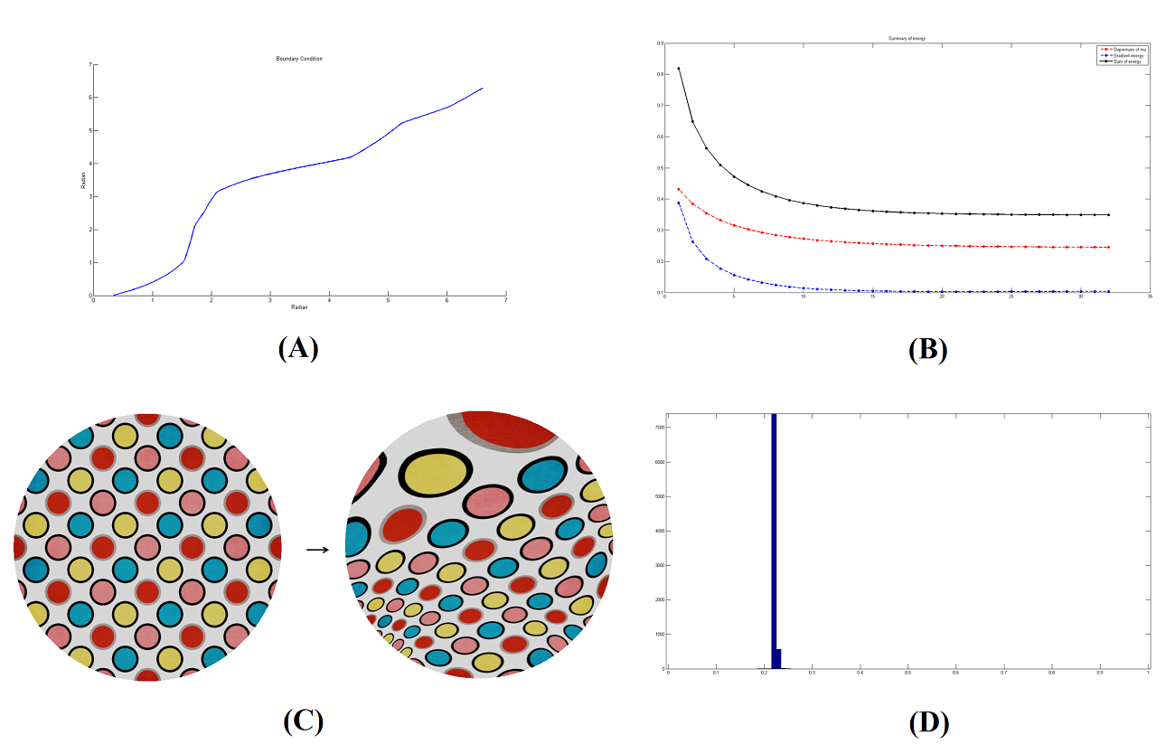
In our first numerical experiment, we test our method to compute the extremal mapping of the disk with a given Dirichlet boundary condition. A Dirchlet condition on the whole boundary is given as shown in Figure 6(A). Using the QC iteration, we iteratively obtain the pair . As shown in Figure 6(B), , and all decrease as iteration increases. The resulting Teichmüller extremal mapping is as shown in Figure 6(C), which is visualized using the texture mapping. Note that the original texture is deformed under the extremal mapping. However, the dilations of the ellipses deformed from the small circles are the same. It means the norm of the BC is constant everywhere. The histogram of the norm of the BC is also shown in Figure 6(D), which again demonstrates the norm of the BC is equal to a constant . The standard deviation of the BC norm is . Note that the Dirichlet boundary condition can be of arbitrary shapes. Figure 7 shows the result of finding the Teichmüller extremal mapping between the disk and the ameba with given boundary conditions. The resultant norm of BC is also constant everywhere, as demonstrated in Figure 7 (B).


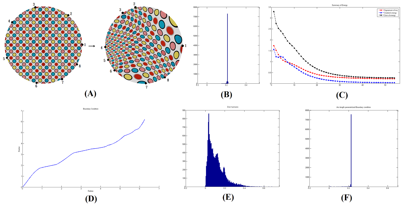
Our algorithm also applies to situation when only a few landmark constraints are enforced on the boundary (instead of the Dirichlet condition defined on the whole boundary). In Figure 8, we test our algorithm to compute Teichmüller extremal mapping of the disk with only 8 landmark points constraints on the boundary. (A) shows the the Teichmüller extremal mapping. Again, the dilations of the ellipses deformed from the small circles are the same, meaning that the norm of the BC is constant everywhere. (B) shows the histogram of the BC norm. The norm of the BC is equal to . (C) shows the energy and the sup-norm of the BC in the QC iteration. Our algorithm also automatically detect the optimal boundary correspondence. (D) shows the obtained optimal boundary correspondence. (E) shows the histogram of the BC norm under harmonic map with arc-length correspondence on the boundary. Note that the distribution of the conformality distortion is highly non-uniform. (F) shows the histogram of the BC norm under the Teichmüller mapping with arc-length parameterized boundary condition (of which the landmark constraints are satisfied). Although a Teichmüller mapping can still be obtained, the norm of the BC is equal to 0.23 which is higher than the case when only 8 points landmark constraints are enforced. Hence, the obtained Teichmüller mapping is not extremal.
6.2 Extremal mapping of multiply-connected domains
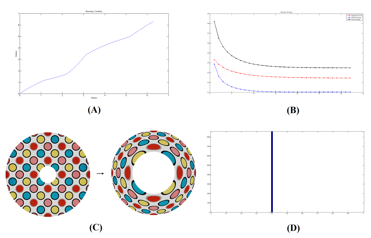
Our method can also be applied to multiply-connected domain. In Figure 9, we test our method to compute the extremal mapping of an annulus with Dirichlet boundary condition. The boundary condition is given in (B). Again, the energy functional is decreasing under the QC iteration. The extremal mapping is as shown in (C). The mapping is a Teichmüller map, since the BC norm is constant everywhere as shown in (D).
Figure 10 and 11 show the results of finding the Teichmüller extremal mapping with 3 and 6 holes respectively. Figure 10 shows the Teichmüller map. The corresponding BC norm, sup-norm of BC and the L2 norm of the gradient of the norm of BC are shown in (B) and (C) respectively. Figure 11 demonstrates the result of a more complicated multiply-connected domain having 6 holes. These results show that our algorithm can again compute the Teichmüller Extremal mapping of multiply-connected domains efficiently and accurately.
6.3 Optimized Teichmüller mapping with interior landmark constraints
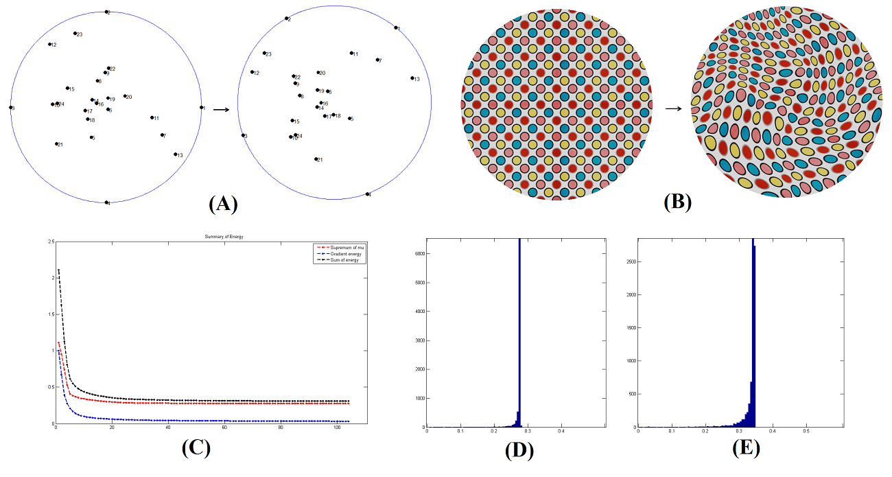
Our algorithm can compute an optimized Teichmüller mapping with interior landmark constraints enforced. Figure 12 shows the optimized Teichmüller mapping between the disk with 25 interior landmark constraints enforced. (A) shows the 24 landmark constraints. (B) shows the obtained Teichmüller mapping, visualized using the texture mapping. (C) shows the energy, the sup-norm of the BC and the L-2 norm of the gradient of the BC in the QC iteration. Note that the sup-norm of the BC decreases during the iteration, which illustrates the mapping converges to an optimal mapping minimizing the conformality distortion. (D) shows the histogram of the norm of the BC. The norm of the BC is uniformly equal to 0.2. (E) shows the histogram of the norm of BC with arc-length boundary correspondence enforced. The norm of the BC is equal to 0.28, which means the Teichmüller mapping is not an extremal one.
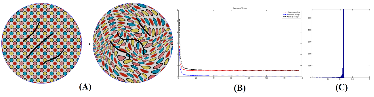
We have test our algorithm to compute the optimized Teichmüller mapping of the disk with 3 interior landmark curves constraints enforced in Figure 13. (A) shows the Teichmüller mapping with 3 landmark curves constraints enforced. (B) shows the energy, the sup-norm of the BC and the L-2 norm of the gradient of the BC in the QC iteration. The energy is decreasing, indicating that the algorithm converges to an optimized Teichmüller mapping. (C) shows the histogram of the norm of the BC. The norm of the BC is accumulated at 0.53.
We also test our algorithm to the case when we only have the correspondence of the interior landmarks. Figure 14 shows an example of finding Teichmüller extremal mapping with 20 interior landmark points only. (A) shows the constraint of the feature points. (B) shows the Teichmüller mapping. (C) shows the histogram of the norm of the BC. It shows that even boundary condition is not provided, our algorithm can still obtain both the Teichmüller extremal mapping which satisfies the landmark constraints and the corresponding optimal boundary condition.
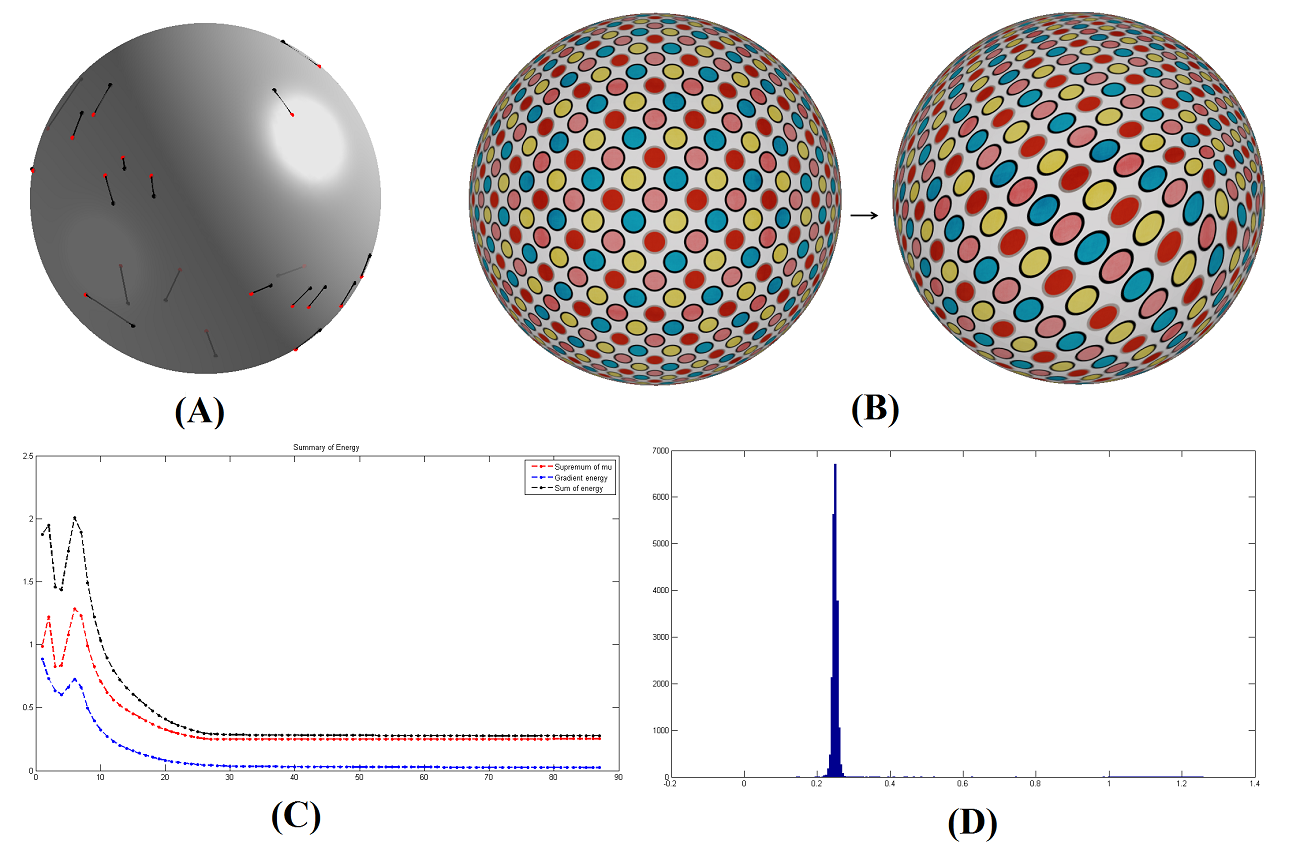
Our algorithm also applies to computing the optimized Teichmüller extremal mapping between the unit sphere with interior landmark constraints enforced. Figure 15 shows an example of Teichmüller extremal mapping with 10 interior landmark constraints enforced. (A) shows landmark constraints on the sphere. (B) shows the Teichmüller mapping. (C) shows the energy, the sup-norm of the BC and the L-2 norm of the gradient of the BC in the QC iteration. Again, the energy is decreasing, indicating that the algorithm converges to an optimized Teichmüller mapping. (D) shows the histogram of the norm of the BC. The norm of the BC is concentrated near 0.21, meaning that the mapping is a Teichmüller mapping.

7 Applications
In this section, we apply our proposed algorithms for computing landmark matching Teichmüller mappings to practical problems. More specifically, we will consider the problems of computing brain landmark matching registrations, constrained texture mappings and human face registrations.
7.1 Brain landmark matching registration
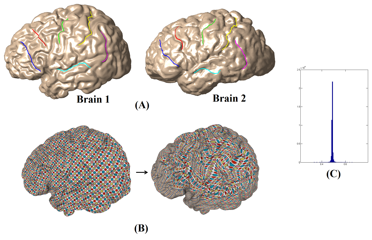
Landmark-based surface registrations are commonly applied for finding meaningful 1-1 correspondences between human brain cortical surfaces. On cortical surfaces, sulcal landmarks can be labeled either manually by neuroscientists or automatically based on various geometric quantities. The sulcal landmarks are important anatomical features. It is therefore desirable to obtain a registration between the cortical surfaces with least geometric distortion, which matches the sulcal landmarks as much as possible. Our algorithms for computing landmark matching Teichmüller mappings can be applied. In Figure 16, we apply our algorithm to compute the Teichmüller mapping between 2 different brain surfaces with 3 corresponding landmarks labeled. (A) shows the corresponding sulcal landmarks, indicated by different colors. (B) shows the obtained Teichmüller extremal mapping with 3 landmark constraints enforced, visualized by the circle packing textures. The sulcal landmarks are exactly matched under the mapping. (C) shows the histogram of the norm of the associated BC. The norm is a constant showing that the obtained registration is indeed a Teichmüller mapping. We also test the method to register cortical surfaces with more sulcal landmarks. In Figure 17, we compute the Teichmüller extremal mapping between 2 brain surfaces with 6 corresponding sulcal landmarks labeled. The obtained registration and the norm of its associated BC is shown in (B) and (C) respectively. The landmarks are exactly matched. Again, the norm of the BC is a constant, showing that the obtained registration is a Teichmüller mapping which minimizes the conformality distortion.

7.2 Constrained texture mapping
Texture mapping is one of the major photorealistic techniques in computer graphics to generate realistic and visually rich 3D surfaces [23, 24]. It is usually done by putting each surface mesh in correspondence with a 2D image [2, 30, 28, 29, 27, 26, 25]. Such a correspondence between the surface mesh and the image is called the texture mapping. Constrained texture mappings are popularly used, in which the texture mappings are guided by landmark features labeled interactively by users. Ideally, the texture mapping should have minimum distortion, while matching the landmark points exactly. We apply our algorithms to compute the landmark matching Teichmüller extremal mapping between the surface mesh and the image, and use it as the texture mapping. In Figure 18, we map a cat image onto the human face surface. (A) shows the corresponding landmark points labeled manually on the human face and the texture image. The landmark matching Teichmüller extremal mapping is computed, and is used as texture mapping to project the cat image onto the human face surface. The textured surface is as shown in (B). (C) shows the norm of the associated BC of the texture mapping. The norm is approximately a constant. It means the texture mapping computed is indeed a Teichmüller extremal mapping, which minimizes the conformality distortion.
In Figure 19, we further test our algorithm on a multiply-connected human face. (A) and (B) shows the texture(tiger) image and a multiply-connected human face. Corresponding landmark points are labeled manually on the texture image and the surface mesh. In (C), the surface mesh is mapped to a multiply-connected domain in 2D by a Teichmüller extremal mapping matching the landmark points exactly. (D) shows the textured surface. (E) shows the norm of the associated BC of the texture mapping. The norm is approximately a constant, which means the texture mapping computed is indeed a Teichmüller extremal mapping.


7.3 Human face registration
In face recognition, finding accurate spatial correspondences between human faces is an a crucial process to compare and recognize faces effectively. Corresponding features can be extracted on human face based on curvatures, such as high curvature points near nose tips and lips. Accurate face registration can then be obtained by computing a mapping that matches the corresponding features. Landmark matching Teichmüller extremal mapping, which minimizes the geometric distortion, can then be used. In Figure 20, we apply our algorithm to compute the registration between a male and female human faces. The human faces are both simply-connected open surfaces. Corresponding feature points are labeled on both faces. The obtained Teichmüller mapping is obtained, which is visualized by texture mapping. The corresponding features are exactly matched. (C) shows the histogram of the norm of the BC, which is almost a constant. This demonstrates the obtained registration is a Teichmüller mapping.

Our algorithm can also be applied to obtain registration between multiply-connected human faces. Figure 21 shows two multiply-connected human faces. Corresponding feature landmarks are labeled. Teichmüller extremal mapping matching the features exactly is computed, as shown in (B). It is again visualized by texture mapping. (C) shows the histogram of the norm of the BC. Again, it is almost a constant, which demonstrates that obtained registration is a Teichmüller mapping minimizing the conformality distortion.

8 Conclusion
We address the problem of computing Teichmüller extremal mapping between surfaces, which minimizes the maximal conformality distortion. The proposed algorithm can be applied to obtain a landmark matching registration between surface meshes. Given a set of corresponding landmark points or curves defined on both surfaces, a unique landmark matching quasi-conformal registration can be obtained, which minimizes the conformality distortion. In this paper, we propose an efficient iterative algorithm, called the Quasi-conformal (QC) iterations, to compute the Teichmüller extremal mapping. The key idea is to represent the set of diffeomorphisms by Beltrami coefficients (BCs). We then look for an optimal BC associated to the desired Teichmüller mapping. The associated diffeomorphism can be efficiently reconstructed from the optimal BC using the Linear Beltrami Solver(LBS). Using our proposed method, the Teichmüller mapping can be accurately and efficiently computed within 10 seconds. The obtained registration is guaranteed to be bijective. Besides, Teichmüller mapping with soft landmark constraints can also be computed using our proposed algorithm. It becomes useful when landmark features cannot be accurately located, and hence it is better to compute registration with landmarks approximately (but not exactly) matched. We applied the proposed algorithm to real applications, such as brain landmark matching registration, constrained texture mapping and human face registration. Experimental results shows that our method is effective in computing a non-overlap landmark matching registration with least amount of conformality distortion.
References
- [1] B. Lévy, S. Petitjean, N. Ray and J. Maillot, Least Squares Conformal Maps for Automatic Texture Atlas Generation, ACM SIGGRAPH conference proceedings, 2002
- [2] E. Zhang, K. Mischaikow and G. Turk, Feature-based surface parameterization and texture mapping, ACM Transactions on Graphics (TOG), Volume 24 Issue 1, January 2005
- [3] S. Haker, S. Angenent, A. Tannenbaum, R. Kikinis, G. Sapiro, and M. Halle. Conformal surface parameterization for texture mapping, IEEE Transaction of Visualization and Computer Graphics, 6:181–189, 2000.
- [4] S.C. Joshi and M.I. Miller, Landmark Matching via Large Deformation Diffeomorphisms, IEEE Transaction on Image Processing, Vol. 9, No. 8, August 2000, pp. 1357-1370.
- [5] F. Gardiner and N. Lakic. Quasiconformal Teichmuller Theory. American Mathematics Society, 2000.
- [6] B. Fischl, M. Sereno, R. Tootell, and A. Dale. High-resolution intersubject averaging and a coordinate system for the cortical surface. Human Brain Mapping, 8:272–284, 1999.
- [7] X. Gu, Y. Wang, T. F. Chan, P. M. Thompson, and S.-T. Yau. Genus zero surface conformal mapping and its application to brain, surface mapping. IEEE Transactions on Medical Imaging, 23(8):949–958, 2004.
- [8] Y. Wang, L. M. Lui, X. Gu, K. M. Hayashi, T. F. Chan, A. W. Toga, P. M. Thompson, and S.-T. Yau. Brain surface conformal parameterization using riemann surface structure. IEEE Transactions on Medical Imaging, 26(6):853–865, 2007.
- [9] X. Gu and S. Yau. Computing conformal structures of surfaces, Communication in Information System, 2(2):121–146, 2002.
- [10] S. Joshi and M. Miller. Landmark matching via large deformation diffeomorphisms. IEEE Transactions on Image Processing, 9(8):1357–1370, 2000.
- [11] M. K. Hurdal and K. Stephenson. Discrete conformal methods for cortical brain flattening, Neuroimage, 45:86–98, 2009.
- [12] Y. Wang, L. Lui, T. Chan, and P. Thompson. Optimization of brain conformal mapping with landmarks. Proceeding in Medical Image Computing and Computer-Assisted Internvention - MICCAI 2005, pages 675–683, 2005.
- [13] L. Lui, S. Thiruvenkadam, Y. Wang, T. Chan, and P. Thompson. Optimized conformal parameterization of cortical surfaces using shape based matching of landmark curves, Proceeding in Medical Image Computing and Computer-Assisted Internvention - MICCAI 2005, pages 494–502, 2008.
- [14] L. Lui, S. Thiruvenkadam, Y. Wang, P. Thompson, and T. Chan. Optimized conformal surface registration with shape-based landmark matching, SIAM Journal of Imaging Sciences, 3(1):52–78, 2010.
- [15] L. Lui, Y. Wang, T. Chan, and P. Thompson. Landmark constrained genus zero surface conformal mapping and its application to brain mapping research, Applied Numerical Mathematics, 57:847–858, 2007.
- [16] L.M. Lui, T.W. Wong, X.F. Gu, T.F. Chan and S.T. Yau. Compression of Surface Diffeomorphism using Beltrami coefficient, IEEE Computer Vision and Pattern Recognition(CVPR), 2839-2846 (2010)
- [17] L.M. Lui, T.W. Wong, W. Zeng, X.F. Gu, P.M. Thompson, T.F. Chan and S.T. Yau. Optimization of Surface Registrations Using Beltrami Holomorphic Flow, Journal of Scientific Computing, DOI 10.1007/s10915-011-9506-2
- [18] L.M. Lui, T.W. Wong, X.F. Gu, P.M. Thompson, T.F. Chan and S.T. Yau. Hippocampal Shape Registration using Beltrami Holomorphic flow, Medical Image Computing and Computer Assisted Intervention(MICCAI), Part II, LNCS 6362, 323-330 (2010)
- [19] W. Zeng, L.M. Lui, F. Luo, T.F. Chan, S.T. Yau, X.F. Gu Computing quasiconformal maps using an auxiliary metric and discrete curvature flow. Numerische Mathematik, 121(4), 671–703, 2012
- [20] L.M. Lui, K.C. Lam, T.W. Wong, X.F. Gu Beltrami Representation and its applications to texture map and video compression. arXiv:1210.8025 (http://arxiv.org/abs/1210.8025)
- [21] O. Lehto and K. Virtanen. Quasiconformal Mappings in the Plane. Springer-Verlag, New York, 1973.
- [22] R. Schoen and S.-T. Yau. Lectures on Differential Geometry. International Press of Boston, 1994.
- [23] J. Foley, A. van Dam, S. Feiner and J. Hughes. Computer Graphics, Addison-Wesley Publishing, Massachusetts, 1992.
- [24] P. S. Heckbert. Survey of texture mapping, IEEE Computer Graphics and Applications 6, No. 11, pages 5667, November 1986.
- [25] L. Balmelli, G. Taubin and F. Bernardini. Space-optimised texture maps, Computer Graphics Forum, 2002, 21, (3), pp. 411420
- [26] C. Bennis, J.M. Vézien and G. Iglésias. Piecewise surface flattening for nondistorted texture mapping, Computer Graphics (SIGGRAPH95 Proceedings) 25, pp 237246, 1991
- [27] S.D. Ma and H. Lin. Optimal texture mapping, EUROGRAPHICS88, pp 421428, September 1988.
- [28] B. Levy and J.L. Mallet. Non-Distorted Texture Mapping for Sheared Triangulated Meshes. Computer Graphics (SIGGRAPH 98 Proceedings), 1998
- [29] B. Levy. Constrained Texture Mapping for Polygonal Meshes. Computer Graphics (SIGGRAPH 98 Proceedings), 28, 2001
- [30] S. Haker, S. Angenent, A. Tannenbaum, R. Kikinis, G. Sapiro, and M. Halle. Conformal surface parameterization for texture mapping. IEEE Transactions on Visualization and Computer Graphics, 6(2), April-June 2000.
- [31] W. Zeng and X. Gu. Registration for 3D Surfaces with Large Deformations Using Quasi-Conformal Curvature Flow. IEEE Conference on Computer Vision and Pattern Recognition (CVPR11), Jun 20-25, 2011, Colorado Springs, Colorado, USA.
- [32] M. Jin, J. Kim, F. Luo and X. Gu. Discrete surface Ricci flow.. IEEE Transaction on Visualization and Computer Graphics, 14(5), 1030–1043, (2008)
- [33] Y.L. Yang, J. Kim, F. Luo, S. Hu, X.F. Gu Optimal Surface Parameterization Using Inverse Curvature Map. IEEE Transactions on Visualization and Computer Graphics , 14(5):1054-1066 (2008)
- [34] W. Zeng, L.M. Lui, L. Shi, D. Wang, W.C. Chu, J.C. Cheng, J. Hua, S.T. Yau, X.F. Gu. Shape Analysis of Vestibular Systems in Adolescent Idiopathic Scoliosis Using Geodesic Spectra. Medica Image Computing and Computer Assisted Intervation 13(3), 538–546 (2010)
- [35] T. Lin, C.L. Guyader, I. Dinov, P. Thompson, A. Toga, L. Vese Gene Expression Data to Mouse Atlas Registration Using a Nonlinear Elasticity Smoother and Landmark Points Constraints. Journal of Scientific Computing, 50(3), 586–609 (2012)
- [36] O. Weber, A. Myles, D. Zorin. Computing Extremal Quasiconformal Maps. Computer Graphics Forum, 31(5), 16791689 (2012)