Belief Propagation Reconstruction for Discrete Tomography

Let us first fix the notations. The image that we want to reconstruct sits on a two-dimensional grid, and each of its $N$ pixels $i$ takes a value in a $q$-ary alphabet: $x_{i}=\chi_{1},\ldots,\chi_{q}$. For instance, binary tomography corresponds to the case where $q=2$, and $\chi_{1}=-1$, $\chi_{2}=1$. We suppose that $M$ tomographic measurements, $\mu=1\ldots M$, have been made. Each such measurement gives a number $y_{\mu}$ which is the sum of variables along a light ray $\mu$:

$$y_{\mu}=\sum_{i\in{\mu}}x_{i}+w_{\mu}$$

(7)

where ${i\in{\mu}}$ denotes the set of all variables $x_{i}$ that belong to the measurement line $\mu$, and $w_{\mu}$ is the additive noise on measure $\mu$. Notice that, in a slightly more general setting, one would measure $y_{\mu}=\sum_{i\in{\mu}}F_{\mu i}x_{i}+w_{\mu}$, where $F_{\mu i}$ is a geometrical factor giving the fraction of pixel $i$ that is covered by the ray corresponding to measurement $\mu$ [45]. This more general setting can be handled as well by our method. Furthermore, it does not make much difference when the image has a structure in domains, as soon as the typical domain size is much larger than one pixel. To keep notations simple we thus keep hereafter to the case where $F_{\mu i}=1$, the straightforward extension to more general cases is left to the reader.

The problem is now to reconstruct the original image (that is the N-dimensional vector ${\mathbf{x}}$) from the values of the projection (the M-dimensional vector ${\mathbf{y}}$).

Here, we shall adopt a Bayesian approach. As a prior information, we use the fact that the image to measure is not a random one, but has a structure in domains, such that if a pixel $i$ has the value $\chi_{r}$, then the neighboring pixel has a large probability to have the same value. We shall enforce this bias in each direction $\mu$ in which a measurement has been made. This is a very natural prior for a large class of images. Following the Bayesian approach, our goal is thus to sample from the a posteriori distribution given by

$\displaystyle P({\mathbf{x}}|{\mathbf{y}})=\frac{P({\mathbf{y}}|{\mathbf{x}})P_{0}({\mathbf{x}})}{P({\mathbf{y}})}=\frac{1}{Z({\mathbf{y}})}{\prod_{\mu}\delta\left({y_{\mu}-\sum_{i\in{\mu}}x_{i}}\right)}P_{0}({\mathbf{x}})$

(8)

where, following the convention in statistical physics, we have rewritten the normalization factor of $P({\mathbf{x}}|{\mathbf{y}})$ as $Z({\mathbf{y}})$. (In the following, we shall incorporate all normalization factors into $Z$.) Here the $\delta$ function implements the equality $y_{\mu}=\sum_{i\in{\mu}}x_{i}$ if the measurement is perfect ($w_{\mu}=0$). In the case of noisy measurement, this $\delta$ function should be smoothed in order to take into account our information on the noise. For instance, when the measurement has Gaussian noise of variance $\Delta$ one could use a function $\delta(x)=\exp(-x^{2}/(2\Delta))/\sqrt{2\pi\Delta}$.

Let us denote by $p_{\mu}$ the a priori probability for neighboring pixels to have the same value along the line $\mu$. Then

	$\displaystyle P_{0}({\mathbf{x}})$	$\displaystyle=$	$\displaystyle\prod_{\mu}\prod_{(ij)\in\mu}p_{\mu}^{\delta_{x_{i},x_{j}}}(1-p_{\mu})^{1-\delta_{x_{i},x_{j}}}=\prod_{\mu}(1-p_{\mu})^{N_{\mu}}\prod_{\mu}e^{\sum_{(ij)\in\mu}\log\left(\frac{p_{\mu}}{1-p_{\mu}}\right)\delta_{x_{i},x_{j}}}$		(9)
		$\displaystyle=$	$\displaystyle{\rm{cst}}\prod_{\mu}e^{\sum_{(ij)\in\mu}J_{\mu}\delta_{x_{i},x_{j}}}$

where $N_{\mu}$ is the number of pixels along line $\mu$, $(ij)\in\mu$ denote pairs of neighboring pixels along direction $\mu$ (for instance, in the case of line $\mu=3$ in Fig.2, there would be an interaction between pixels (i) and (ii) and another one between (ii) and (iii)) and $\rm{cst}$ is a constant that does not depend on the values of the variables, and that we shall thus incorporate into the normalization factor through a redefinition of $Z({\mathbf{y}})$. In (9) we have introduced the so-called “coupling constant” $J_{\mu}=\log{\frac{p_{\mu}}{1-p_{\mu}}}$.

With these notations, the a posteriori probability can thus be written as a product of $M$ terms, each corresponding to one tomographic projection:

$\displaystyle P({\mathbf{x}}|{\mathbf{y}})=\frac{1}{Z}\prod_{\mu=1}^{M}\left[\delta\left(y_{\mu}-\sum_{i\in{\mu}}x_{i}\right)e^{J_{\mu}\sum_{(ij)\in\mu}\delta_{x_{i},x_{j}}}\right]$

(10)

The value of $J_{\mu}$ can be fixed based on previous knowledge of the spatial structure of the sample. It would also be possible to learn its value in the course of the algorithm, by maximizing the probability of $J_{\mu}$ given the measures $\mathbf{y}$ (this amounts to maximizing the partition function $Z$ in Eq. (10)). This can be done for instance using the Expectation Maximization approach [46].

Sampling from the distribution in Eq. (8) is a notoriously difficult problem [10, 8]. We shall here use an approach based on a message-passing algorithm called “Belief-Propagation” (BP) [47, 48, 49, 50]. It is not an exact algorithm (at least for the present problem), in the sense that it is not guaranteed to sample correctly from the distribution (8). However, we shall see that the approximate sampling obtained from BP performs empirically very well.

Let us first reformulate the problem as a graphical model [47, 50]. We have $N$ variables $x_{i}$ and $M$ factor nodes, each one implementing the weight $\delta(y_{\mu}-\sum_{i\in\mu}x_{i})e^{J_{\mu}\sum_{(ij)\in\mu}x_{i} x_{j}}$. The corresponding factor graph is shown in Fig. 2.

We shall not review here the derivation of the belief-propagation algorithm, and refer instead to classical books and articles on the subject [49, 50]. There are essentially two equivalent ways to derive the BP recursion: one is to see it as a recursion that would be exact if the factor graph were a tree (i.e. if it had no loop). Another one is to see it as an Ansatz in the usual variational Bayesian inference approach that usually improves on the factorized ”mean-field” one, leading to an expression for the log-likelihood whose maximization leads to the belief-propagation equations. The result is a set of message passing equations relating messages that go from variables to nodes and from nodes to variables. The message $m_{i\to\gamma}$ from a variable $i$ to a node $\gamma$ is the marginal probability of the variable $x_{i}$ in absence of the constraint $\gamma$ (see Fig. 3). On the other hand, the message $\tilde{m}_{\mu\to i}$ from the factor $\mu$ to the variable $i$ is the marginal probability of the variable $x_{i}$ when only constraint $\mu$ is present (see Fig. 3). The message $m_{i\to\gamma}$ is easily written in terms of the messages $\tilde{m}_{\mu\to i}$:

$$m_{i\to\gamma}(x_{i})\propto\prod_{\mu\in i\neq\gamma}\tilde{m}_{\mu\to i}(x_{i})$$

(11)

where $\mu\in i$ denotes all the factor nodes (tomographic lines) that contain variable $i$. Note that $m_{i\to\gamma}(x_{i})$ should be normalized , in the sense that $\sum_{x}m_{i\to\gamma}(x)=1$ (we prefer however not to write explicitly the normalisation factor and will therefore use the sign $\propto$ instead of $=$). The message from a factor node to a variable, on the other hand, reads:

$\displaystyle\tilde{m}_{\mu\to i}(x_{i})$

$\displaystyle\propto$

$\displaystyle\sum_{x_{j};j\in\mu\neq i}\delta(y_{\mu}-\sum_{j\in\mu}x_{j})e^{J_{\mu}\sum_{(jk)\in\mu}\delta_{x_{j},x_{k}}}\prod_{j\in\mu\neq i}m_{j\to\mu}(x_{j})$

(12)

Equations (11) and (12) build a closed set of equations that should be solved for the values of the messages. Usually one seeks a solution by iterating these equations starting from some randomly chosen initial condition. Assuming that a fixed point of this iteration is reached, one obtains a set of messages that solve the BP equations. The BP estimate for the marginal distribution of $x_{i}$ is then given by

$$m_{i}(x_{i})\propto\prod_{\mu\in i}\tilde{m}_{\mu\to i}(x_{i})$$

(13)

Let us now take a closer look at the recursion: While the iteration from variables to factors (in eq. (11)) is easy to compute (a simple multiplication), the one from nodes to variables (in eq. (12)) is unfortunately more complicated, as it involves a sum over all the $q$ possible values of each variable $x$ in the line ${\mu}$. Moreover, we have to do it for each of the $N_{\mu}$ variables in this line, and for each value it can take. At first sight, this seems to give a complexity of order $N_{\mu}q^{N_{\mu}}$ for each iteration. However, one can compute the message in (12) in a much more efficient way, namely in $O(qN_{\mu})$ iterations. Indeed, in physics language, one can recognize that estimating $\tilde{m}_{\mu\to i}(x_{i})$ in Eq. (12) is nothing else that estimating the marginal of $x_{i}$ in a one-dimensional graphical model known in physics as the Potts ferromagnet in a random field at fixed total magnetization, which can be done efficiently by transfer matrix techniques, which are equivalent for this problem to using BP. The solution is thus to use BP in order to compute the messages of the initial BP problem.

Let us now focus on the following sub-problem: we want to estimate the marginal of a variable $x_{i}$ coupled in a chain of $N_{\mu}$ variables, with a statistical weight given by

$$P_{\mu\to i}({\mathbf{x}})\propto\delta(y_{\mu}-\sum_{j\in\mu}x_{j})e^{J_{\mu}\sum_{(jk)\in\mu}\delta_{x_{j},x_{k}}}\prod_{j\in\mu\neq i}m_{j\to\mu}(x_{j})\,.$$

(14)

There are two methods to deal with the delta function which we shall refer to (using the statistical physics language) as the ”canonical method” and the ”micro-canonical method”. The exact solution is to use the microcanonical method where one is indeed summing only over the configurations of the variables that satisfy the delta function in Eq. (14). This can be done efficiently using a transfer matrix approach, and we have thus implemented this method. It turns out, however, that the canonical method is faster. It is also a more natural approach when there exist errors or noise in the measurement process. We shall therefore use the latter method in the following.

The canonical method amounts to relaxing the $\delta(y_{\mu}-\sum_{j\in\mu}x_{j})$ constraint, and treating it only as an approximate constraint that should hold on average, up to some small fluctuations. More precisely, in the canonical method we replace the delta function using a Lagrange multiplier $H$ (the ”field” in physics language) that we shall fix later on in order to enforce the constraint on average. The statistical weight thus becomes, instead of (14):

$$P^{H}_{\mu\to i}({\mathbf{x}})\propto e^{-H(y_{\mu}-\sum_{j\in\mu}x_{j})}e^{J_{\mu}\sum_{(jk)\in\mu}\delta_{x_{j},x_{k}}}\prod_{j\in\mu\neq i}m_{j\to\mu}(x_{j})\,,.$$

(15)

The value of $H$ is computed using $\mathbb{E}^{H}(\sum_{j\in\mu}x_{j})=y_{\mu}$, where $\mathbb{E}^{H}$ denotes the expectation value with respect to the measure $P^{H}$. Of course, the value of $H$ depends on both $\mu$, and $i$. Now, it turns out that one can compute $H$ with an error that becomes negligible (in the limit where the number of variables involved in the measurement $\mu$ is large), by considering the complete problem obtained from (15) by including all the messages $m_{j\to\mu}$. This complete problem is defined by:

$$P^{H}_{\mu}({\mathbf{x}})\propto e^{-H(y_{\mu}-\sum_{j\in\mu}x_{j})}e^{J_{\mu}\sum_{(jk)\in\mu}\delta_{x_{j},x_{k}}}\prod_{j\in\mu}m_{j\to\mu}(x_{j})\,.$$

(16)

We now write the nested belief propagation equations for this complete sub-problem. Since the interaction is a two-body one, one can write it using a version that involves only one type of message, from variables to variables (see [51, 50] and Fig. 4). It is also equivalent to the so-called transfer matrix approach in statistical mechanics [50]. The recursion for the BP messages is easily written. In order to keep notations simple, let us assume that the numbering of variables is such that variable $i$ is neighbour to $i+1$ along direction $\mu$. We shall denote the messages going from right to left of the line as the right-moving messages $\eta^{R}_{i\to i-1}({x_{i}})$, $i=2,\dots,N_{\mu}$ and the ones going from left to right as the left-moving messages $\eta^{L}_{i\to i+1}({x_{i}})$, $i=1,\dots,N_{\mu}-1$ (see Fig. 4). $\eta^{R}_{i\to i-1}({x_{i}})$ is the marginal of $x_{i}$ in the absence of the left part of the chain beyond $x_{i}$. Then one has (for the left-moving messages):

	$\displaystyle\eta^{L}_{i\to i+1}({x_{i}})$	$\displaystyle=$	$\displaystyle\frac{m_{i\to\mu}(x_{i})}{Z}e^{Hx_{i}}\left[\eta^{L}_{i-1\to i}({x_{i}})e^{J_{\mu}}+\sum_{x_{i-1}\neq x_{i}}\eta^{L}_{i-1\to i}({x_{i-1}})\right]$		(17)
		$\displaystyle=$	$\displaystyle\frac{m_{i\to\mu}(x_{i})}{Z}e^{Hx_{i}}\left[1+\eta^{L}_{i-1\to i}({x_{i}})(e^{J_{\mu}}-1)\right]\,,$

where we have used that $\sum_{x_{i}}\eta^{L}_{i\to i+1}({x_{i}})=1$ and $Z$ is the corresponding normalization factor. The recursion for the right-moving messages is similar, with the $i+1$ and $i-1$ playing reverse roles.

Once all the $\eta^{L}$ and $\eta^{R}$ are computed, one can then obtain the desired $\tilde{m}_{\mu\to i}(x_{i})$, taking care of the fact that the message $m_{i\to\mu}(x_{i})$ should not be included (see eq. 12), using

$$\tilde{m}_{\mu\to i}(x_{i})=\frac{e^{Hx_{i}}}{Z}\left[1+\eta^{L}_{i-1\to i}({x_{i}})(e^{J_{\mu}}-1)\right]\left[1+\eta^{R}_{i+1\to i}({x_{i}})(e^{J_{\mu}}-1)\right]\,,$$

(18)

where $Z$ is again a normalization.

Finally, the expected value of the variable $y_{\mu}=\sum_{i\in{\mu}}x_{i}$ can be computed using the average value of $x_{i}$ in presence of the random field (and this time therefore including the term $m_{i\to\mu}$) given by

$$\mathbb{E}(x_{i})=\frac{\sum_{x_{i}}x_{i}\tilde{m}_{\mu\to i}(x_{i})m_{i\to\mu}(x_{i})}{\sum_{x_{i}}\tilde{m}_{\mu\to i}(x_{i})m_{i\to\mu}(x_{i})}\,,$$

from which we can compute the expected value of the sum of the variables $M(H)$ along the line $\mu$:

$$M(H)=\mathbb{E}\left(\sum_{i\in{\mu}}x_{i}\right)=\sum_{i\in{\mu}}\mathbb{E}(x_{i})\,.$$

(19)

A standard result of statistical physics is that $M(H)$ is a monotonous function of $H$. This is a consequence of the fact that there are no phase transitions in a one-dimensional Potts model [52, 53]. This means that one can apply safely a dichotomy algorithm to find the value of $H$ such that $y_{\mu}=M(H)$.

With the canonical method, one cannot fix exactly $\sum_{i\in{\mu}}x_{i}$ but rather its expectation, and this means that we are allowing fluctuations (typically of order $O(\sqrt{y_{\mu}})$) around the strict tomographic constraint. Of course, one might also want to enforce strictly this constraint, in which case one has to resort to the microcanonical method.

Given these equations, the complete marginals for each variable can be computed using Eq. (13). The marginal $m_{i}(x_{i})$ denotes the probability that variable $i$ is assigned the value $x_{i}$; and the most likely labeling is thus given, at each step of the algorithm, by

$$x_{i}^{*}=\rm{argmax}_{x_{i}}m_{i}(x_{i}).$$

(20)

After convergence of the algorithm, the values $x_{i}^{*}$ thus represent the segmentation into discrete labels that is looked for.

We shall now specialize for the rest of this paper to binary tomography, that is, the case $q=2$, where the variables take values $x_{i}=-1,1$ (after a suitable rescaling of experimental data) ¹¹ 1 Even if the exact values of the discrete levels are not known, a method for estimating the discrete values has been proposed by Batenburg et al. [54]. In physics terminology, this amounts to the Ising model, and we shall sometimes use the term “spins” for pixels. In this case, it is convenient to rewrite the expressions in a simpler way. Indeed, for binary variables $x$ one can write a probability using a real variable $h$ (which we will call the field) via:

$$P(x)=\frac{e^{hx}}{2\cosh{h}}\,.$$

(21)

Therefore, we define the fields $h_{i\to\mu}$ and $\tilde{h}_{\mu\to i}$ by

	$\displaystyle m_{i\to\mu}(x_{i})=\frac{e^{h_{i\to\mu}x_{i}}}{2\cosh{{h_{i\to\mu}}}}\,,$		(22)
	$\displaystyle\tilde{m}_{\mu\to i}(x_{i})=\frac{e^{\tilde{h}_{\mu\to i}x_{i}}}{2\cosh{{\tilde{h}_{\mu\to i}}}}.$		(23)

Using this notation, we can rewrite the message from a variable to a node eq. (11) as follows:

$$h_{i\to\gamma}=\sum_{\mu\in i\neq\gamma}\tilde{h}_{\mu\to i}\,.$$

(24)

The message from a node to a variable, on the other hand, reads:

	$\displaystyle\tilde{m}_{\mu\to i}(x_{i})$	$\displaystyle\propto$	$\displaystyle\sum_{x_{j};j\in\mu\neq i}\delta(y_{\mu}-\sum_{j\in\mu}x_{j})e^{J_{\mu}\sum_{(jk)\in\mu}x_{j} x_{k}}\prod_{j\in\mu\neq i}m_{j\to\mu}(x_{j})$		(25)
		$\displaystyle\propto$	$\displaystyle\sum_{x_{j};j\in\mu\neq i}\delta(y_{\mu}-\sum_{j\in\mu}x_{j})e^{J_{\mu}\sum_{(jk)\in\mu}x_{j} x_{k}+\sum_{j\in\mu\neq i}x_{j}h_{j \to\mu}}\,.$		(26)

The marginal $\tilde{m}_{\mu\to i}(x_{i})$ thus corresponds to the one of a one-dimensional random field Ising model, where the external fields are given by $h_{j \to\mu}$, and constrained to have a total magnetization $y_{\mu}$. The recursion “within a line” (corresponding to Eq. (17) in the general case) can also be written in terms of fields, using $\eta^{L}(x)=\frac{e^{u^{L}x}}{2\cosh{u^{L}}}$ and $\eta^{R}(x)=\frac{e^{u^{R}x}}{2\cosh{u^{R}}}$, we have

	$\displaystyle u^{L}_{i\to i+1}={\rm{atanh}}{\left[\tanh{J_{\mu}}\tanh{(H+h_{i\to\mu}+u^{L}_{i-1\to i})}\right]}\,,$		(27)
	$\displaystyle u^{R}_{i\to i-1}={\rm{atanh}}{\left[\tanh{J_{\mu}}\tanh{(H+h_{i\to\mu}+u^{R}_{i+1\to i})}\right]}\,.$		(28)

Again, once these are computed, the marginal can be expressed as

	$\displaystyle\tilde{m}_{\mu\to i}(x_{i})=\frac{e^{\tilde{h}_{\mu\to i}x_{i}}}{2\cosh{{\tilde{h}_{\mu\to i}}}}\,,$		(29)
	$\displaystyle{\tilde{h}_{\mu\to i}}=u^{L}_{i-1\to i}+u^{R}_{i+1\to i}+H\,.$		(30)

Finally, the expected value of the variable $y_{\mu}=\sum_{i\in{\mu}}x_{i}$, that is needed to fix the correct value of $H$, is given by summing the average value of $x_{i}$ (with all random fields), each of them given by

$$\mathbb{E}(x_{i})=\tanh{(h_{i \to\mu}+\tilde{h}_{\mu\to i})}\,,$$

(31)

which is the analog of eq. (3.3) for the binary case. Finally, the most likely assignment for the values $x_{i}$ at each step of the algorithm is given by

$$x_{i}^{*}=\rm{sign}\left(\tanh{\sum_{\mu\in i}\tilde{h}_{\mu\to\char 16\relax}}\right)=\rm{sign}\left(\sum_{\mu\in i}\tilde{h}_{\mu\to\char 16\relax}\right).$$

(32)

We shall now summarize the complete algorithm for the binary case. Let us start by a few comments about the practical implementation.

• •

  An efficient way to initialize the fields $\tilde{h}_{\mu\to i}$ is to compute their equilibrium value for $J=0$:

  $$\tilde{h}_{\mu\to i}={\rm{atanh}}\left(y_{\mu}/N_{\mu}\right),$$

  (33)

  where $N_{\mu}$ is the number of variables on the line $\mu$. This initialization is also used in [44].

• •

  Along a light ray slanted with respect to the pixel grid, the distance between successive spins can be larger than 1. In this case, we use a coupling between the spins that decreases when the distance between neighbors increases. We use $J_{\mu}={\rm{atanh}}\left(\tanh^{D}{J}\right)$ where $D$ is the $\ell_{1}$ distance (Manhattan or taxi-cab distance) between successive variables on the line $\mu$. This choice, suggested by the so-called high-temperature approximation [55], mimics the effective correlation between two variables at distance $D$ in the two-dimensional Ising model.

• •

  We have observed that the results $x_{i}^{*}$ depend only weakly on the value of $J$, as long as $J=O(1)$. Hence, we did not optimize the value of $J$: all the results presented here were obtained with $J=0.2$.

• •

  In the case of noise-free measures, we stop the algorithm when all line-sums constraints are satisfied by the $x_{i}^{*}$. For noisy measures, we stop the algorithm when the number of flipping spins saturates; this criterion is discussed in Sec. 5.

• •

  We have observed empirically that damping the update of the fields is sometimes necessary for a proper convergence of the algorithm. We thus replaced eq.(30) by

  $${\tilde{h}_{\mu\to i}}^{t+1}=s{\tilde{h}_{\mu\to i}}^{t}+(1-s)\left(u^{L}_{i-1\to i}+u^{R}_{i+1\to i}+H\right)\,.$$

  (34)

  In our implementation, we have fixed empirically the damping value $s$ to $1-1.6/n_{\theta}$. This scaling was found to ensure convergence for all the values of $n_{\theta}$ and $N$ tested.

• •

  In order to avoid overflow or underflow problems, we clip the value of the different fields inside an interval $[-B,B]$. We set $B$ to 400, a value large enough for the result to be independent of $B$.

• •

  In order to find the value of the external field $H$, a few dichotomy iterations are enough to find $H$ up to a good precision $\epsilon$ (we use $\epsilon=0.05$). In order to speed up the computation of $H$, we use Newton’s method when the total magnetization is close enough to $y_{\mu}$.

$\textnormal{BP-TOMO}(y_{\mu},{\rm criterion},t_{\rm max})$
  1Initialize the messages $\tilde{h}$ as described above. 2while ${\rm conv}>{\rm criterion}$ and $t<t_{\rm max}$: 3 do 4 $t\leftarrow t+1$. 5 for each ${\mu};i\in\mu$: 6 doUpdate $h_{i\to\mu}$ according to eq. (24). 7 for each ${\mu};i\in\mu$: 8 do 9 while $\left(\left|y_{\mu}-\sum_{i\in\mu}\mathbb{E}\left(x_{i}\right)\right|<\epsilon\right)$ 10 doCompute the messages $u^{L}$ and $u^{R}$ according to eq. (27-28). 11 Compute the new value of $\sum_{i\in{\mu}}\mathbb{E}\left(x_{i}\right)$, update $H$ (e.g. by dichotomy). 12 Update the $\tilde{h}_{\mu\to i}$ according to eq. (34). 13 doCompute the new values $x_{i}^{*}$ from eq.(32) and check for convergence. 14return signal components $x_{i}^{*}$. Note that this algorithm is of the embarrassingly parallel type, since each line $\mu$ can be handled separately when computing line $7$ in the above pseudo-code. This could be used to speed up the algorithm by solving each line separately on different cores. A Python code (with some C extensions) of the current version is available on https://github.com/eddam/bp-for-tomo, under a free-software BSD license.

In order to measure the performance of our algorithm, we generate synthetic images with different levels of sparsity of the gradients, but a similar binary microstructure. We obtain such a set of images with a controlled level of gradient sparsity as follows: $p^{2}$ pixels are picked at random inside the image and set to $1$ while the background is set to $0$, then a Gaussian filter of width proportional to $1/p$ is applied to the image. The resulting continuous-valued image is finally thresholded at the mean intensity to obtain a binary image. Examples of binary images with different values of $p$ are shown in Fig. 5. A simple measure of the sparsity of our images is given by

$$\rho(x)=\frac{\ell(x)}{N},$$

(35)

where $\ell(x)$ is the length of the internal boundary of one of the two phases in the image. The internal boundary is the set of pixels that have within their 4-connected neighbours at least one pixel belonging to the other phase ²² 2 The internal boundary can be computed by simple mathematical morphology operations [56], as the difference between the origin image and its morphological erosion. Morphological erosion is one of the two fundamental operations in mathematical morphology [56], realizing the intuitive idea of eroding binary sets from their boundaries.. $\rho$ therefore measures the fraction of pixels lying on the boundary. We choose this measure since the original image can be retrieved from the knowledge of the internal boundary (and the value of a single pixel). It would also have been possible to choose the set of pixels for which the finite-differences gradient of the image is non-zero. However, the latter set of pixels is redundant for retrieving the image, and leads to a slight over-estimation of the sparsity of the image. Using the definition of Eq. (35), we find that $\rho$ scales linearly with $p$.

Let us first investigate the effect of the number of angles on the reconstruction of a given image, when no noise is added to the projections: $\mathbf{y}=\mathbf{F}\mathbf{x}$. We define the undersampling rate by the ratio between the number of measures and the number of variables:

$$\alpha=\frac{M}{N}.$$

(36)

Since belief propagation is not an exact algorithm, it is not guaranteed to reconstruct the exact original image. Nevertheless, we find experimentally that for a sufficient number of measures, the algorithm always reconstructs the exact image after a finite number of iterations. Once all spins have reached the correct orientation, we observe that their orientation does not change any more. For a given image, the evolution of the discrepancy between the segmentation of the magnetization (Eq. (32)) and the ground truth is plotted in Fig. 6 (a) against the number of iterations, for different measurement rates $\alpha$. The number of errors decays roughly exponentially with time, but the decay rate increases with the number of measurements: the convergence towards the exact image is faster when more measurements are available. Also, a sharp transition is observed for a critical $\alpha$, under which the number of errors does not reach zero, and eventually increases again at long times. The transition between the two regimes is hard to estimate accurately, since the convergence time seems to diverges when the transition is approached, as shown in Fig. 6 (b). We estimate the critical undersampling rate from the lowest number of angles for which exact reconstruction is reached before 400 iterations.

We have measured the critical undersampling rate $\alpha_{c}$ for images with different sizes of the microstructure, hence different levels of sparsity. The critical undersampling rate is plotted against the boundary density $\rho$ (Eq. (35)) in Fig. 6 (c). We observe a linear relationship

$$\alpha_{c}\simeq\rho.$$

(37)

This simple relationship corresponds to a very good recovery performance, since $\rho N$ can be seen as the number of unknowns needed to retrieve the image. Therefore, we only need a number of measurements $M=\alpha N$ comparable to the number of unknowns for an exact reconstruction of the image.

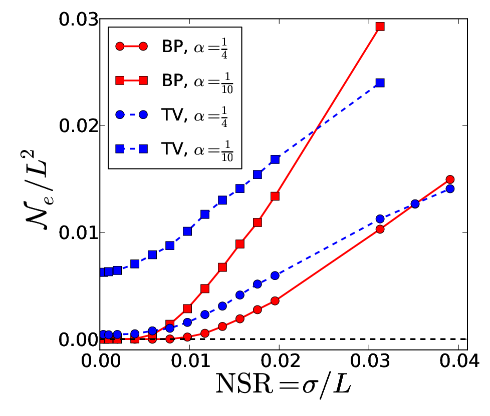
In Fig. 8, we have plotted the reconstruction error for the same image against the measure noise to signal ratio, for two values of the measurement rate $\alpha=1/4$ and $\alpha=1/10$. An image with $p=14$ (Fig. 5 left) was used, and $J=0.2$ was used for all values of the NSR. We have also computed the reconstruction error for the convex minimization of Eq. (6). For a fair comparison, the best value of $\beta$ minimizing the reconstruction error was computed using Brent’s method (whereas no parameter was optimized for BP-tomo). We observe that the reconstruction quality is better for BP-tomo than for the convex algorithm, up to a threshold above which the error is greater for BP-tomo. For the smaller undersampling rate $\alpha=1/10$, the values of the error reached at the threshold are too high for a satisfying reconstruction for several applications (most pixels lying on boundaries are wrongly labeled). Interestingly, there is a first regime for small noise, for which the fraction of errors is zero or very small for BP-tomo, while the error increases much faster for the convex algorithm. For large noise, however, the convex algorithm gives better results.

Fig. 9 shows that the reconstruction errors are mostly located on the boundaries between the two phases for the two algorithms (except for a few isolated errors for BP-tomo), but that a larger fraction of the interfaces are correctly reconstructed for BP-tomo. Fig. 9 also displays the continuous magnetization, as well as the non-segmented minimization of the convex algorithm. We see that the contours of the objects are delineated more accurately for BP-tomo than for the convex algorithm, especially for objects with concavities.

For a given value of the NSR, we observe in Fig. 8 that the reconstruction error increases when the measurement rate decreases. The effect of the measurement rate in the noisy case is studied in the next paragraph.

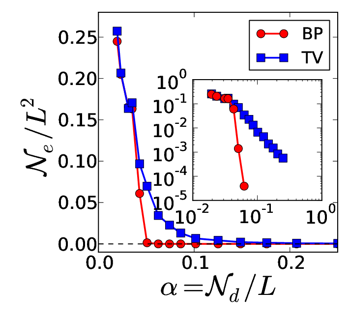
For the same image ($p=14$, $J=0.2$), we have fixed the SNR to $0.002$ and computed the reconstruction error as a function as the measurement rate, for the two algorithms. Results are shown in Fig. 10. For BP-tomo, we observe a sharp transition between an exact reconstruction to a failed reconstruction when the measurement rate is decreased (a score of 0.5 would be obtained when labeling pixels at random). Therefore, the noisy case displays a transition between failure and success as in the noise-free case (Fig. 6). The transition is observed at the same measurement rate as the noise-free case. Approaching the transition from above, a finite error fraction appears (see the log-log inset in Fig. 10). In the noise-free case, exact reconstruction could be reached until the transition, but an increasing number of iterations was needed when approaching the transition (Fig. 6 (b)).

In contrast, the evolution of the error fraction when decreasing the measurement rate is much smoother for the convex algorithm, and does not display a phase transition in Fig. 10. As a result, the error fraction is larger for the convex algorithm above the BP-tomo transition. At low measurement rates, the error fraction is comparable for the two algorithms, but this regime corresponds to values of the error fraction that are not acceptable for most applications.

For a larger value of the noise, Fig. 11 shows that a transition between good and failed reconstruction is still observed. However, the fraction of errors is larger, therefore the transition is not as sharp as for smaller NSR. Comparing Fig. 10 and Fig. 11, we conclude that the reconstruction quality is better above the transition for a SNR of $0.01$ than for the convex algorithm for a SNR five times smaller.

References

- [1] M. Slaney and A. Kak. Principles of computerized tomographic imaging. SIAM, Philadelphia, 1988.
- [2] G.T. Herman. Fundamentals of Computerized Tomography: Image Reconstruction from Projections. Springer Verlag, 2009.
- [3] L.A. Shepp and B.F. Logan. The Fourier reconstruction of a head section. IEEE Trans. Nucl. Sci, 21(3):21–43, 1974.
- [4] GN Ramachandran and AV Lakshminarayanan. Three-dimensional reconstruction from radiographs and electron micrographs: application of convolutions instead of Fourier transforms. PNAS, 68(9):2236–2240, 1971.
- [5] J. Baruchel, J.Y. Buffiere, P. Cloetens, M. Di Michiel, E. Ferrie, W. Ludwig, E. Maire, and L. Salvo. Advances in synchrotron radiation microtomography. Scripta Materialia, 55(1):41–46, 2006.
- [6] J.Y. Buffiere, E. Maire, J. Adrien, J.P. Masse, and E. Boller. In situ experiments with X-ray tomography: an attractive tool for experimental mechanics. Experimental mechanics, 50(3):289–305, 2010.
- [7] R. Gordon, R. Bender, and G.T. Herman. Algebraic reconstruction techniques (ART) for three-dimensional electron microscopy and x-ray photography. Journal of theoretical Biology, 29(3):471–481, 1970.
- [8] G.T. Herman and A. Kuba, editors. Discrete Tomography: Foundations, Algorithms, and Applications. Birkhäuser, 2009.
- [9] K.J. Batenburg and J. Sijbers. DART: A practical reconstruction algorithm for discrete tomography. Image Processing, IEEE Transactions on, 20(9):2542–2553, 2011.
- [10] B. Carvalho, G. Herman, S. Matej, C. Salzberg, and E. Vardi. Binary tomography for triplane cardiography. In Information Processing in Medical Imaging, volume 1613 of Lecture Notes in Computer Science, pages 29–41. Springer Berlin / Heidelberg, 1999.
- [11] E.Y. Sidky and X. Pan. Image reconstruction in circular cone-beam computed tomography by constrained, total-variation minimization. Physics in medicine and biology, 53:4777, 2008.
- [12] Y. Boykov, O. Veksler, and R. Zabih. Fast approximate energy minimization via graph cuts. Pattern Analysis and Machine Intelligence, IEEE Transactions on, 23(11):1222–1239, 2001.
- [13] R.J. Gardner. Geometric tomography, volume 2006. Cambridge University Press Cambridge, 1995.
- [14] R.J. Gardner and P. McMullen. On Hammer’s X-ray problem. Journal of the London Mathematical Society, 2(1):171, 1980.
- [15] K. Batenburg, W. Fortes, L. Hajdu, and R. Tijdeman. Bounds on the difference between reconstructions in binary tomography. In Discrete Geometry for Computer Imagery, pages 369–380. Springer, 2011.
- [16] R. Aharoni, GT Herman, and A. Kuba. Binary vectors partially determined by linear equation systems. Discrete Mathematics, 171(1):1–16, 1997.
- [17] H.Y. Liao and G.T. Herman. Automated estimation of the parameters of gibbs priors to be used in binary tomography. Discrete applied mathematics, 139(1):149–170, 2004.
- [18] H.Y. Liao and G.T. Herman. A coordinate ascent approach to tomographic reconstruction of label images from a few projections. Discrete applied mathematics, 151(1):184–197, 2005.
- [19] H.Y. Liao and G.T. Herman. A method for reconstructing label images from a few projections, as motivated by electron microscopy. Annals of Operations Research, 148(1):117–132, 2006.
- [20] A. Mohammad-Djafari. Gauss-markov-potts priors for images in computer tomography resulting to joint optimal reconstruction and segmentation. International J. of Tomography and Statistics (IJTS), 11:76–92, 2008.
- [21] A.H. Delaney and Y. Bresler. Globally convergent edge-preserving regularized reconstruction: an application to limited-angle tomography. Image Processing, IEEE Transactions on, 7(2):204–221, 1998.
- [22] S. Weber, C. Schnorr, and J. Hornegger. A linear programming relaxation for binary tomography with smoothness priors. Electronic Notes in Discrete Mathematics, 12:243–254, 2003.
- [23] T. Schüle, C. Schnörr, S. Weber, and J. Hornegger. Discrete tomography by convex–concave regularization and DC programming. Discrete Applied Mathematics, 151(1):229–243, 2005.
- [24] S. Weber, A. Nagy, T. Schüle, C. Schnörr, and A. Kuba. A benchmark evaluation of large-scale optimization approaches to binary tomography. In Discrete Geometry for Computer Imagery, pages 146–156. Springer, 2006.
- [25] S. Weber, T. Schüle, A. Kuba, and C. Schnörr. Binary tomography with deblurring. Combinatorial Image Analysis, pages 375–388, 2006.
- [26] S. Weber, T. Schüle, J. Hornegger, and C. Schnörr. Binary tomography by iterating linear programs from noisy projections. Combinatorial Image Analysis, pages 38–51, 2005.
- [27] E.J. Candès, J. Romberg, and T. Tao. Robust uncertainty principles: Exact signal reconstruction from highly incomplete frequency information. Information Theory, IEEE Transactions on, 52(2):489–509, 2006.
- [28] E.J. Candes, J.K. Romberg, and T. Tao. Stable signal recovery from incomplete and inaccurate measurements. Communications on pure and applied mathematics, 59(8):1207–1223, 2006.
- [29] D.L. Donoho. Compressed sensing. Information Theory, IEEE Transactions on, 52(4):1289–1306, 2006.
- [30] S.P. Boyd and L. Vandenberghe. Convex optimization. Cambridge Univ Pr, 2004.
- [31] P.L. Combettes and J.C. Pesquet. Proximal splitting methods in signal processing. Fixed-Point Algorithms for Inverse Problems in Science and Engineering, pages 185–212, 2011.
- [32] J. Song, Q.H. Liu, G.A. Johnson, and C.T. Badea. Sparseness prior based iterative image reconstruction for retrospectively gated cardiac micro-CT. Medical physics, 34(11):4476, 2007.
- [33] GT Herman and R. Davidi. Image reconstruction from a small number of projections. Inverse Problems, 24:045011, 2008.
- [34] J. Tang, B.E. Nett, and G.H. Chen. Performance comparison between total variation (tv)-based compressed sensing and statistical iterative reconstruction algorithms. Physics in Medicine and Biology, 54:5781, 2009.
- [35] E.Y. Sidky, M.A. Anastasio, and X. Pan. Image reconstruction exploiting object sparsity in boundary-enhanced X-ray phase-contrast tomography. Optics Express, 18(10):10404–10422, 2010.
- [36] X. Jia, Y. Lou, R. Li, W.Y. Song, and S.B. Jiang. Gpu-based fast cone beam ct reconstruction from undersampled and noisy projection data via total variation. Medical physics, 37:1757, 2010.
- [37] S. Anthoine, J. Aujol, Y. Boursier, and C. Melot. On the efficiency of proximal methods in cbct and pet. In Image Processing (ICIP), 2011 18th IEEE International Conference on, pages 1365–1368. IEEE, 2011.
- [38] N. Pustelnik, C. Chaux, and J. Pesquet. Parallel proximal algorithm for image restoration using hybrid regularization. Image Processing, IEEE Transactions on, (99):1–1, 2009.
- [39] N. Pustelnik, C. Chaux, J.C. Pesquet, and C. Comtat. Parallel algorithm and hybrid regularization for dynamic pet reconstruction. In Nuclear Science Symposium Conference Record (NSS/MIC), 2010 IEEE, pages 2423–2427. IEEE, 2010.
- [40] H. Raguet, J. Fadili, and G. Peyré. Generalized forward-backward splitting. Arxiv preprint arXiv:1108.4404, 2011.
- [41] A. Beck and M. Teboulle. Fast gradient-based algorithms for constrained total variation image denoising and deblurring problems. Image Processing, IEEE Transactions on, 18(11):2419–2434, 2009.
- [42] GR Myers, TE Gureyev, DM Paganin, and SC Mayo. The binary dissector: phase contrast tomography of two-and three-material objects from few projections. Optics express, 16(14):10736–10749, 2008.
- [43] K.J. Batenburg. A network flow algorithm for reconstructing binary images from discrete X-rays. Journal of Mathematical Imaging and Vision, 27(2):175–191, 2007.
- [44] S. Roux, H. Leclerc, and F. Hild. Tomographic reconstruction of binary fields. In Journal of Physics: Conference Series, volume 386, page 012014. IOP Publishing, 2012.
- [45] P.M. Joseph. An improved algorithm for reprojecting rays through pixel images. Medical Imaging, IEEE Transactions on, 1(3):192–196, 1982.
- [46] A.P. Dempster, N.M Laird, and D.B. Rubin. Maximum likelihood from incomplete data via the em algorithm. Journal of the Royal Statistical Society, 38:1, 1977.
- [47] J. Pearl. Reverend bayes on inference engines: A distributed hierarchical approach. In Proceedings American Association of Artificial Intelligence National Conference on AI, pages 133–136, Pittsburgh, PA, USA, 1982.
- [48] F. R. Kschischang, B. Frey, and H.-A. Loeliger. Factor graphs and the sum-product algorithm. IEEE Trans. Inform. Theory, 47(2):498–519, 2001.
- [49] J.S. Yedidia, W.T. Freeman, and Y. Weiss. Understanding belief propagation and its generalizations. In Exploring Artificial Intelligence in the New Millennium, pages 239–236. Morgan Kaufmann, San Francisco, CA, USA, 2003.
- [50] M. Mézard and A. Montanari. Information, Physics, and Computation. Oxford Press, Oxford, 2009.
- [51] L. Zdeborová and F. Krzakala. Phase transitions in the coloring of random graphs. Phys. Rev. E, 76:031131, Sep 2007.
- [52] Gabor T. Herman and Attila Kuba. Mathematical Physics in One Dimension: ExactlySoluble Models of Interacting Particless. Academic Press, 1966.
- [53] L D Landau and E M Lifshitz. Statistical Physics. Pergamon, 1959.
- [54] KJ Batenburg, W. van Aarle, and J. Sijbers. A semi-automatic algorithm for grey level estimation in tomography. Pattern Recognition Letters, 32(9):1395–1405, 2011.
- [55] R. P. Feynman. Statistical Mechanics: A Set of Lectures. Fontrier in Physics, 1972.
- [56] J. Serra. Image analysis and mathematical morphology. London.: Academic Press., 1982.
- [57] S.J. Tu, C.C. Shaw, and L. Chen. Noise simulation in cone beam ct imaging with parallel computing. Physics in medicine and biology, 51:1283, 2006.
- [58] D. Donoho and J. Tanner. Observed universality of phase transitions in high-dimensional geometry, with implications for modern data analysis and signal processing. Philosophical Transactions of the Royal Society A: Mathematical, Physical and Engineering Sciences, 367(1906):4273–4293, 2009.
- [59] D.L. Donoho and J. Tanner. Precise undersampling theorems. Proceedings of the IEEE, 98(6):913–924, 2010.
- [60] F. Krzakala, M. Mézard, F. Sausset, Y. F. Sun, and L. Zdeborová. Statistical-physics-based reconstruction in compressed sensing. Phys. Rev. X, 2:021005, May 2012.
- [61] F. Krzakala, M. Mézard, F. Sausset, Y. Sun, and L. Zdeborová. Probabilistic reconstruction in compressed sensing: algorithms, phase diagrams, and threshold achieving matrices. Journal of Statistical Mechanics: Theory and Experiment, 2012(08):P08009, 2012.
- [62] L. Chaari, S. Mériaux, S. Badillo, J.-Ch. Pesquet, and P. Ciuciu. Multidimensional wavelet-based regularized reconstruction for parallel acquisition in neuroimaging. EURASIP Journal on Advances in Signal Processing, December 2011. Under revision.