Sequentiality and Adaptivity Gains in
Active Hypothesis Testing

Here, we provide a precise formulation for the active $M$-ary hypothesis testing problem.

Let $\Omega=\{1,2,\ldots,M\}.$ Let $H_{i}$, $i\in\Omega$, denote $M$ hypotheses of interest among which only one holds true. Let $\theta$ be the random variable that takes the value $\theta=i$ on the event that $H_{i}$ is true for $i\in\Omega$. We consider a Bayesian scenario with a given prior (belief) about $\theta$, i.e., initially $P(\{\theta=i\})=\rho_{i}(0)>0$ for all $i\in\Omega$. $\mathcal{A}$ is the set of all sensing actions and is assumed to be finite with $|\mathcal{A}|=K<\infty$. $\mathcal{Z}$ is the observation space. For all $a\in\mathcal{A}$, the observation kernel $q^{a}_{i}(\cdot)$ (on $\mathcal{Z}$) is the probability density function for observation $Z$ when action $a$ has been taken and $H_{i}$ is true. We assume that observation kernels $\{q^{a}_{i}(\cdot)\}_{i,a}$ are known. Let $L$ denote the penalty for a wrong declaration, i.e., the penalty of selecting $H_{j}$, $j\neq i$, when $H_{i}$ is true. Let $\tau$ be the (stopping) time at which the decision maker retires. The objective is to find a stopping time $\tau$, a sequence of sensing actions $A(0),A(1),\ldots,A({\tau-1})$, and a declaration rule $d:~\mathcal{A}^{\tau}\times\mathcal{Z}^{\tau}\to\Omega$ that collectively minimize the expected total cost

where the expectation is taken with respect to the initial belief as well as the distribution of observation sequence.

Note that in the above problem, the cost of a test is stated in terms of minimizing the expected sample size plus the expected penalty of wrong declaration. We are interested in the characterization of this cost as a function of penalty $L$. It is easy to show that under the optimal selection rule, the probability of error approaches zero as $L$ approaches infinity. Furthermore, as shown in [20], the above problem is (asymptotically) equivalent to the problem of minimizing the (expected) number of samples subject to a constraint $\epsilon=(L\log L)^{-1}$ on the expected probability of error.

A policy is a rule based on which stopping time $\tau$ and sensing actions $A(t)$, $t=0,1,\ldots,\tau-1$ are selected. We assume that sensing actions are selected according to randomized decision $\boldsymbol{\lambda}\in\Lambda(\mathcal{A})$ whose element $\lambda_{a}$ indicates the probability of selecting sensing action $a$ and in general might change with time or not. The sensing actions and the stopping time can be selected either based on the past observation outcomes or independent from them. According to this fact, policies are divided into four categories based on the following two factors: i) sequential vs. non-sequential; ii) adaptive vs. non-adaptive. Non-sequential policies collect a fixed number of observation samples and make the final decision afterwards; while under sequential policies, the sample size is not known initially and is determined by the observation outcomes. More precisely, under non-sequential policies, $\tau=N$ for some $N\in\mathbb{N}$; while for sequential policies, $\tau$ is a random stopping time. Under adaptive policies, the decision maker relies on the previous collected samples to select the next sensing action; while under non-adaptive policies, the actions are selected independent of the past observation outcomes.

The problem of active $M$-ary hypothesis testing is a partially observable Markov decision problem (POMDP) where the state is static and observations are noisy. It is known that any POMDP is equivalent to an MDP with a compact yet uncountable state space, for which the belief of the decision maker about the underlying state becomes an information state [21]. In our setup, thus, the information state at time $t$ is nothing but a belief vector specified by the conditional probability of hypotheses $H_{1},H_{2},\ldots,H_{M}$ to be true given the initial belief and all the previous observations and actions. Let $\boldsymbol{\rho}(t)$ denote the posterior belief after $t$ observations. Accordingly, the information state space is defined as $\mathbb{P}(\Theta)=\big\{{\boldsymbol{\rho}}\in[0,1]^{M}:\sum_{i=1}^{M}\rho_{i}=1\big\}$ where $\Theta$ is the $\sigma$-algebra generated by random variable $\theta$. In one sensing step, the evolution of the belief vector follows Bayes’ rule and the expected total cost (1) can be rewritten as

where ${\bar{\text{Pe}}}=\mbox{\boldlarge E}[1-\max_{j\in\Omega}\rho_{j}(\tau)]$ is the probability of wrong declaration and the expectations are taken with respect to the distribution of observation sequence as well as the prior distribution on $\theta$.

Let $V_{NN}(\boldsymbol{\rho})$, $V_{SN}(\boldsymbol{\rho})$, $V_{SA}(\boldsymbol{\rho})$, and $V_{NA}(\boldsymbol{\rho})$, denote the minimum expected total cost (2) for prior belief $\boldsymbol{\rho}$ under non-sequential non-adaptive, sequential non-adaptive, sequential adaptive, and non-sequential adaptive policies, respectively.

Active hypothesis testing generalizes the passive (classical) hypothesis testing problem where the number of sensing actions is limited to one, both in the fixed sample size (non-sequential) case [14, 15, 22] as well as the sequential one [11, 12, 13]. While the fixed sample size studies have primarily focused on the asymptotic analysis in form of identifying error exponents for various error types [14, 15, 22], the study of sequential hypothesis testing has come in form of identifying the expected optimal sample size to achieve a given error probability.

The generalization to the active testing case was considered by Chernoff in [1] in which a decision maker controls sensing actions to optimize the expected total cost (1) in a sequential (variable sample size) setting. In particular, in [1] and its extensions [23, 20, 18], heuristic sequential adaptive randomized policies were proposed and were shown to be asymptotically optimal as $L\to\infty$ where the notion of asymptotic optimality [1] denotes the relative tightness of the performance upper bound associated with the proposed policy and the lower bound associated with the optimal policy.¹¹ 1 In [1], the objective was to minimize $c\mathbb{E}[\tau]+{\bar{\text{Pe}}}$ and the proposed policy was shown to be asymptotically optimal as $c\to 0$. It is straightforward to show that for $L=\frac{1}{c}$, this problem coincides with the active hypothesis testing problem defined in this paper. However, we have chosen $\mathbb{E}[\tau]+L{\bar{\text{Pe}}}$ as an objective function here because of its Lagrangian relaxation interpretation of an information acquisition problem in which the objective is to minimize $\mathbb{E}[\tau]$ subject to ${\bar{\text{Pe}}}\leq\epsilon$ where $\epsilon>0$ denotes the desired probability of error.

The general active binary hypothesis testing problem was recently studied in [16, 17] where full characterization of the error exponent corresponding to the class of adaptive and non-adaptive policies was provided. In particular, the error exponent corresponding to these two classes was shown to be equal, hence establishing zero adaptivity gain among non-sequential policies. The generalization to $M>2$ was considered in [18]. Note that while [18] fully characterizes the error exponent corresponding to non-sequential non-adaptive policies; it provides only a partial characterization of (i.e., loose upper and lower bounds on) the error exponent corresponding to non-sequential adaptive policies.

Table I provides a visual summary of the literature on hypothesis testing, excluding the authors’ prior work, as discussed above.

We close our literature survey with an overview of the main contributions of this paper, which expands our previous works [24, 23, 25, 20] and unifies various aspects of the prior work:

• •

  We provide asymptotically tight lower and upper bounds on $V_{NN}(\boldsymbol{\rho})$, $V_{SN}(\boldsymbol{\rho})$, and $V_{SA}(\boldsymbol{\rho})$ which hold uniformly for all prior $\boldsymbol{\rho}\in\mathbb{P}(\Theta)$.

  • –

    The asymptotic tight bounds on $V_{NN}(\boldsymbol{\rho})$ relies on the analysis of [14, 15] and the realization that in order to minimize the total cost, we have to decrease the error probabilities of various types with the same exponent among the worst pair of hypotheses. Since unlike the passive case studied in [14, 15], the non-adaptive policies produce non-iid observation samples, the final step is to characterize the relationship between the error exponent of a fixed block length and one-step error exponent.

  • –

    The asymptotic tight bounds on $V_{SN}(\boldsymbol{\rho})$ extend the results obtained by [13] to the Bayesian context while allowing for randomized non-adaptive policies. More specifically, the result of [13] is obtained via the law of large numbers and only holds if the observations are i.i.d. Since observations are not identical (although they are independent), different proof technique is required (note that unlike the non-sequential case of extending the work of [14, 15], the random nature of sample size in the sequential case does not allow for a predetermined relationship between the error exponent of a fixed block and one-step error exponent).

  • –

    The asymptotic tight bounds on $V_{SA}(\boldsymbol{\rho})$ extend those obtained by Chernoff [1] to the Bayesian context while relaxing the assumption on uniform discrimination of hypotheses or the need for the infinitely often reliance on randomized action deployed in [18] to ensure sufficient discrimination among hypotheses.

• •

  In addition, we partially characterize a lower bound for $V_{NA}(\boldsymbol{\rho})$. This is, in the Bayesian context, similar to the partial characterization of error exponent of [18].

• •

  As corollaries to the above performance bounds, we characterize the sequentiality gain and adaptivity gain in terms of $L$. In particular, it is shown that the sequentiality gain grows logarithmically as the penalty $L$ increases. We also state a simple necessary and sufficient condition ensuring a logarithmic adaptivity gain in $L$ for the active binary hypothesis testing case.

• •

  Furthermore, primarily as a sanity check, Section IV-B contains the maximum achievable error exponents $E_{NN}$, $E_{SN}$, and $E_{SA}$ in the Bayesian context. In particular, our result regarding $E_{NN}$ coincides with that of [16, 17, 18]; while the result regarding $E_{SA}$ coincides with that of [1, 18] in the Bayesian context. To the best of our knowledge, the result on $E_{SN}$ is new and has not been established before; while our upper bound on $E_{NA}$ is subsumed by the analysis in [18].

Throughout the paper, we have the following technical Assumptions.

Assumption 1 ensures the possibility of discrimination between any two hypotheses. Assumption 2 implies that no two hypotheses are fully distinguishable using a single observation sample.

To continue with our analysis, we need the following definitions and notations.

These notions of discrimination and reliability, as we will see, are natural (and Bayesian) extensions of reliability in classical detection [22] where reliability function for hypothesis $i$ is related to type $i$ error probability. The following fact enables a concrete relationship between these notions.

In this subsection, we provide upper and lower bounds on the minimum expected total cost (1) under different types of policies defined in Subsection II-B. These bounds will be used then in Section IV to characterize the gains of sequential and adaptive selection of actions.

We close this section by a note on the class of non-sequential adaptive policies even though they seem rather unnatural to us (It is more reasonable to control the sample size using the observation outcomes if they are already being used to select sensing actions). Next proposition provides a lower bound on the minimum expected total cost under non-sequential adaptive policies, denoted by $V_{NA}$.

Next we state and discuss the consequences of the bounds proposed above. In Subsection IV-A, we focus on the advantages of causally selecting the retire/declaration time as well as the adaptive selecting of sensing actions. In Subsection IV-B, we derive the error exponent corresponding to different types of policies.

In this subsection, we discuss the advantage of causally selecting the retire/declaration time, i.e., $\tau$ as well as the sensing actions. Let $V_{NN}$, $V_{SN}$, and $V_{SA}$, respectively, denote the minimum expected total cost under non-sequential non-adaptive, sequential non-adaptive, and sequential adaptive policies under uniform prior, i.e., $V_{x}:=V_{x}([\frac{1}{M},\frac{1}{M},\ldots,\frac{1}{M}])$ where $x$ denotes the class of policies $NN$, $SN$, and $SA$.

First, we show that the performance gap between the sequential and non-sequential policy, $V_{NN}-V_{SN}$, grows logarithmically as the penalty $L$ increases. We refer to this performance gap as the sequentiality gain.

Next, the advantage of adaptively selecting the sensing actions is discussed. In particular, it is shown that the performance gap between the adaptive and non-adaptive policy, $V_{SN}-V_{SA}$, grows logarithmically as the penalty $L$ increases. We refer to this performance gap as the adaptivity gain.

A sufficient condition under which there is no adaptivity gain is that of stochastic dominance/degradation [27], i.e., if there exists a stochastic transformation $W$ from $\mathcal{Z}$ to $\mathcal{Z}$ and²² 2 Function $W:\mathcal{Z}\times\mathcal{Z}\to\mathbb{R_{+}}$ is called a stochastic transformation from $\mathcal{Z}$ to $\mathcal{Z}$ if it satisfies $\int_{\mathcal{Z}}W(y;z)dz=1$. a sensing action $a^{*}$ such that for all other sensing actions $a\in\mathcal{A}$,

As shown by Sakaguchi [28], (16) implies that

hence, ensuring zero adaptivity gain when observations obtained by all actions are stochastically degraded version of the observation under sensing action $a^{*}$. This formalizes the notion of informativeness and confirms the conjecture provided in [5].

Let $\mathbb{E}^{\pi}[\tau]$ denote the expected stopping time (or equivalently the expected number of collected samples) under policy $\pi$. Policy $\pi$ is said to achieve error exponent $E>0$ if

where $\text{Pe}^{\pi}(t,M)$ is the smallest probability of error that policy $\pi$ can guarantee when looking for the true hypothesis among $M$ hypotheses with $\mathbb{E}^{\pi}[\tau]\leq t$ (Note that for non-sequential policies, $\tau$ is deterministic).

Next we use the bounds obtained in Section III to characterize the maximum achievable error exponent for different type of policies. Let $E_{NN}$, $E_{SN}$, $E_{SA}$, and $E_{NA}$ denote the maximum achievable error exponent under non-sequential non-adaptive, sequential non-adaptive, sequential adaptive, and non-sequential adaptive policies.

We can also find an upper bound on the maximum achievable error exponent of any non-sequential yet adaptive policy (tight lower bounds are necessary for full characterization, however).

The performance bounds provided in Section III are simplified by substituting the following equations into the denominators of the bounds.

Next we state a simple necessary and sufficient condition for a logarithmic adaptivity gain in the active binary hypothesis testing case.

The problem of passive binary hypothesis testing ($K=1$, $M=2$) with fixed-length (non-sequential) as well as variable-length (sequential) sample size has been studied by [14, 29, 22, 18]. Our sequentiality gain, in this case, is the manifestation of the fact that “sequential tests are superior in ensuring that both error probabilities decreasing at the best possible exponential rates” [29].

Recently, the authors in [16] and [17] have studied the problem of active binary hypothesis testing for fixed-length and variable-length sample size respectively. Our work complements the findings in [17] by providing an asymptotic optimal solution in a total cost (and Bayesian) sense as well as establishing a non-zero sequentiality and potentially non-zero adaptivity gain. In [16], the error exponent corresponding to the class of NN and NA policies were fully characterized for the problem of active binary hypothesis testing with fixed sample size. In the Bayesian context, the result of [16] regarding the error exponent of the class of NN policies coincides with our Corollary 6, while the full characterization of the error exponent corresponding to the class of NA policies in [16], strengthens Corollary 7 in the binary case. In particular, it is shown that in the binary hypothesis testing setup $E_{NN}=E_{NA}$, hence, establishing zero adaptivity gain among non-sequential policies. For the special case of channel coding with feedback³³ 3 The problem of channel coding with feedback can be interpreted as a special case of active hypothesis testing (See [30] for more details). with two messages, the above result, i.e., the zero adaptivity gain among non-sequential policies, was established in [31, 32].

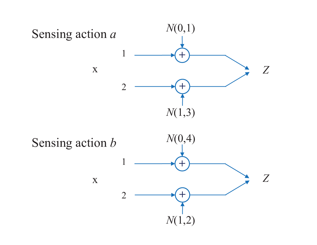
Consider the active binary hypothesis testing problem with additive Gaussian noisy observations under two actions $a$ and $b$ shown in Fig. 1. In this example, the observation noise associated with actions $a$ and $b$ are such that they add unequal noise to the hypotheses. In the remainder of this subsection, we compare the performance of all considered policies for this example.

Table II compares the performance bounds of the considered policies for the example of Fig.1.

In this subsection, we show that

where

Suppose $\hat{\boldsymbol{\lambda}}\in\Lambda(\mathcal{A})$ achieves the maximum in (20). Let $\pi_{NN}$ be a non-sequential non-adaptive policy that collects $\hat{n}$ observation samples and selects sensing actions according to the randomized rule $\hat{\boldsymbol{\lambda}}$. The expected total cost under this policy is $\hat{n}+L{\bar{\text{Pe}}}$. Next we find an upper bound for ${\bar{\text{Pe}}}$. Let $\mathcal{Z}_{i}(n)=\left\{Z^{n}:\rho_{i}(n)\geq\rho_{j}(n)\text{ for all }j\in\Omega\right\}$ and $e_{ij}(n)=P(\{Z^{n}:\rho_{i}(n)<\rho_{j}(n)\}|\theta=i)$.

From (21) and Lemma 1 in Appendix -E, we obtain

We can select $\hat{n}$ as

such that ${\bar{\text{Pe}}}=O(\frac{1}{L})$, and hence,

This completes the proof of upper bound. Next the proof of lower bound is given.

Consider a policy $\pi_{NN}$ that collects $n$ observation samples according to $\boldsymbol{\lambda}\in\Lambda(\mathcal{A})$. We have

From (23) and Lemma 1 in Appendix -E, a lower bound is obtained for the expected total cost under policy $\pi_{NN}$. The lower bound for $V_{NN}$ is obtained by minimizing over the choices of $n$ and $\boldsymbol{\lambda}$.

In this subsection, we show that

In contrast to the passive case, the observations in the active case (either adaptive or non-adaptive) are not necessarily identical over time. Therefore the analysis of [13] for sequential passive hypothesis testing (which is based on the law of large number and results for random walks) is not applicable to the problem of sequential non-adaptive hypothesis testing.

Suppose $\hat{\boldsymbol{\lambda}}\in\Lambda(\mathcal{A})$ achieves the minimum in (24). The upper bound (24) is achieved by a policy that selects sensing actions according to $\hat{\boldsymbol{\lambda}}$ and stops sampling at

Let $\tau_{i}$, $i\in\Omega$, be Markov stopping times defined as follows:

Note that by definition

This implies that $\rho_{i}(\tau_{i})\geq 1-L^{-1}$ and hence, $\tau\leq\tau_{i}$ for all $i\in\Omega$. From (2), total cost under the above policy can be written as

where $\boldsymbol{\rho}=[\rho_{1},\rho_{2},\ldots,\rho_{M}]=[\rho_{1}(0),\rho_{2}(0),\ldots\rho_{M}(0)]$ and the last inequality follows from the fact that $\tau\leq\tau_{i}$, $\forall i\in\Omega$.

Next we find an upper bound for $\mathbb{E}[\tau_{i}|\theta=i]$, $i\in\Omega$. Before we proceed, we introduce the following notation to facilitate the proof:

Let $\iota:=(\log L)^{-\frac{1}{4}}$. We have

References

- [1] H. Chernoff, “Sequential design of experiments,” The Annals of Mathematical Statistics, vol. 30, pp. 755–770, 1959.
- [2] P. Shenoy and A. J. Yu, “Rational decision-making in inhibitory control,” Frontiers in Human Neuroscience, vol. 5, no. 48, 2011.
- [3] M. V. Burnashev, “Data transmission over a discrete channel with feedback. Random transmission time,” Problemy Peredachi Informatsii, vol. 12, no. 4, pp. 10–30, 1975.
- [4] G. Thatte, U. Mitra, and J. Heidemann, “Parametric methods for anomaly detection in aggregate traffic,” IEEE/ACM Transactions on Networking, vol. 19, no. 2, pp. 512–525, April 2011.
- [5] G. A. Hollinger, U. Mitra, and G. S. Sukhatme, “Active classification: theory and application to underwater inspection,” 2011, available on arXiv:1106.5829.
- [6] R. D. Nowak, “The geometry of generalized binary search,” IEEE Transactions on Information Theory, vol. 57, no. 12, pp. 7893–7906, December 2011.
- [7] C. L. Chan, P. H. Che, S. Jaggi, and V. Saligrama, “Non-adaptive probabilistic group testing with noisy measurements: Near-optimal bounds with efficient algorithms,” in 49th Annual Allerton Conference on Communication, Control, and Computing, 2011, pp. 1832–1839.
- [8] A. O. Hero and D. Cochran, “Sensor management: past, present, and future,” IEEE Sensors Journal, vol. 11, no. 12, pp. 3064–3075, December 2011.
- [9] M. Malloy and R. Nowak, “Sequential analysis in high-dimensional multiple testing and sparse recovery,” in IEEE International Symposium on Information Theory (ISIT), 2011, pp. 2661–2665.
- [10] M. A. Iwen, “Group testing strategies for recovery of sparse signals in noise,” in Forty-Third Asilomar Conference on Signals, Systems and Computers, 2009, pp. 1561–1565.
- [11] A. Wald and J. Wolfowitz, “Optimal character of the sequential probability ratio tests,” The Annals of Mathematical Statistics, vol. 19, no. 3, pp. 326–339, 1948.
- [12] P. Armitage, “Sequential analysis with more than two alternative hypotheses, and its relation to discriminant function analysis,” Journal of the Royal Statistical Society, Series B, vol. 12, no. 1, pp. 137–144, 1950.
- [13] G. Lorden, “Nearly-optimal sequential tests for finitely many parameter values,” The Annals of Statistics, vol. 5, no. 1, pp. 1–21, 1977.
- [14] R. E. Blahut, “Hypothesis testing and information theory,” IEEE Transactions on Information Theory, vol. 20, no. 4, pp. 405–417, July 1974.
- [15] E. Tuncel, “On error exponents in hypothesis testing,” IEEE Transactions on Information Theory, vol. 51, no. 8, pp. 2945–2950, August 2005.
- [16] M. Hayashi, “Discrimination of two channels by adaptive methods and its application to quantum system,” IEEE Transactions on Information Theory, vol. 55, no. 8, pp. 3807–3820, August 2009.
- [17] Y. Polyanskiy and S. Verdu, “Hypothesis testing with feedback,” in Information Theory and Applications Workshop (ITA), 2011.
- [18] S. Nitinawarat, G. Atia, and V. V. Veeravalli, “Controlled sensing for multihypothesis testing,” 2012, available on arXiv:1205.0858.
- [19] ——, “Controlled sensing for hypothesis testing,” in IEEE International Conference on Acoustics, Speech, and Signal Processing (ICASSP), March 2012.
- [20] M. Naghshvar and T. Javidi, “Active sequential hypothesis testing,” 2012, available on arXiv:1203.4626.
- [21] P. R. Kumar and P. Varaiya, Stochastic systems: estimation, identification, and adaptive control. Prentice-Hall, Inc., 1986.
- [22] E. A. Haroutunian, M. E. Haroutunian, and A. N. Harutyunyan, Reliability criteria in information theory and in statistical hypothesis testing. Hanover, MA, USA: Now Publishers Inc., January 2007, vol. 4, no. 2.
- [23] M. Naghshvar and T. Javidi, “Performance bounds for active sequential hypothesis testing,” in IEEE International Symposium on Information Theory (ISIT), 2011, pp. 2666–2670.
- [24] ——, “Information utility in active sequential hypothesis testing,” in Proceedings of the 48th Allerton conference on communication, control, and computing, 2010.
- [25] ——, “Active hypothesis testing: sequentiality and adaptivity gains,” in Conference on Information Sciences and Systems (CISS), March 2012.
- [26] O. Shayevitz, “On Rényi measures and hypothesis testing,” in IEEE International Symposium on Information Theory (ISIT), 2011, pp. 894–898.
- [27] D. Blackwell, “Equivalent comparisons of experiments,” The Annals of Mathematical Statistics, vol. 24, pp. 265–272, 1953.
- [28] M. Sakaguchi, “Information theory and decision making,” 1964, unpublished lecture notes, Statistic Deptartment, The George Washington University, Washington, D.C.
- [29] I. Csiszár and P. Shields, Information theory and statistics: a tutorial. Now Publishers Inc., December 2004, vol. 1, no. 4.
- [30] M. Naghshvar and T. Javidi, “Variable-length coding with noiseless feedback and finite messages,” in Conference Record of the Forty Fourth Asilomar Conference on Signals, Systems and Computers, 2010, pp. 317–321.
- [31] E. R. Berlekamp, “Block coding with noiseless feedback,” 1964, PhD Thesis, MIT, Cambridge, MA.
- [32] B. Nakiboglu, “Exponential bounds on error probability with feedback,” 2011, PhD Thesis, MIT, Cambridge, MA.
- [33] M. V. Burnashev, “Sequential discrimination of hypotheses with control of observations,” Math. USSR Izvestija, vol. 15, no. 3, pp. 419–440, 1980.
- [34] V. Bentkus, “An extension of the hoeffding inequality to unbounded random variables,” Lithuanian Mathematical Journal, vol. 48, no. 2, pp. 137–157, 2008.
- [35] V. P. Dragalin, A. G. Tartakovsky, and V. V. Veeravalli, “Multihypothesis sequential probability ratio tests. I. Asymptotic optimality,” IEEE Transactions on Information Theory, vol. 45, no. 7, pp. 2448–2461, November 1999.
- [36] N. Vaidhiyan, S. Arun, and R. Sundaresan, “Active sequential hypothesis testing with application to a visual search problem,” in IEEE International Symposium on Information Theory (ISIT), 2012, pp. 2201–2205.
- [37] P. Billingsley, Probability and measure. John Wiley & Sons, Inc., 1995.
- [38] C. McDiarmid, “On the method of bounded differences,” Surveys in Combinatorics, London Mathematical Society Lecture Note Series 141, Cambridge University Press, pp. 148–188, 1989.