Power Spectrum Precision for Redshift Space Distortions
Abstract
Redshift space distortions in galaxy clustering offer a promising technique for probing the growth rate of structure and testing dark energy properties and gravity. We consider the issue of to what accuracy they need to be modeled in order not to unduly bias cosmological conclusions. Fitting for nonlinear and redshift space corrections to the linear theory real space density power spectrum in bins in wavemode, we analyze both the effect of marginalizing over these corrections and of the bias due to not correcting them fully. While naively subpercent accuracy is required to avoid bias in the fixed case, in the fitting approach the Kwan-Lewis-Linder reconstruction function for redshift space distortions is found to be accurately selfcalibrated with little degradation in dark energy and gravity parameter estimation for a next generation galaxy redshift survey such as BigBOSS.
I Introduction
The pattern of galaxy clustering in three dimensions, and its evolution, encodes abundant information on the cosmological parameters affecting matter growth. Ongoing and next generation spectroscopic galaxy surveys will vastly increase our measurements of this clustering, and our knowledge of cosmology if we can accurately interpret the results in terms of theory. Measurements accrue an extra contribution to the redshift, and hence apparent position along the sight, from the galaxy peculiar velocities induced by the inhomogeneous density field; this gives rise to an anisotropy in the observed clustering known as redshift space distortions (RSD).
These distortions carry information on the growth rate, as opposed to just the growth amplitude, and so are valuable for probing cosmology, as well as the gravitational strength driving the growth. However, linear theory is insufficient for accurate relation of the redshift space galaxy power spectrum to the true (real space) matter density power spectrum, even on quite large scales, or wavenumbers /Mpc, where the vast majority of the statistical leverage lies [1, 2, 3, 4, 5, 6]. Numerous corrections involving higher order perturbation theory have been employed [7, 8, 9, 10] that extend the validity but the region /Mpc is still problematic, especially for quantities involving the growth rate and the gravitational growth characterization. For example, [6] demonstrates that these first principles approaches deliver results for the growth rate that are biased by several standard deviations when using modes out to /Mpc.
Here we investigate a basic question: how accurately does one actually need to know the redshift space distortion mapping in order to extract the cosmological and gravitational parameter information without substantial bias or degradation? Similar questions have been considered for weak gravitational lensing, for example, where one asks how well the nonlinear matter power spectrum needs to be known to estimate cosmology from the lensing shear power spectrum [11, 12].
In Section II we introduce the correction, or reconstruction, function for the redshift space power spectrum and review the KLL [6] form for it. Section III uses the Fisher bias method to compute both the individual parameter bias and joint confidence contour bias due to misestimated RSD, thus giving criteria for the accuracy to which the RSD effects must be known. Adding fit parameters for uncertainties in the reconstruction function in Sec. IV, we assess the impact of marginalizing over them on the cosmological parameters, in particular for tests of dark energy and gravity. Section V summarizes the results and conclusions.
II Galaxy Power Spectrum
II.1 Redshift Space Power Spectrum
In real space the matter density power spectrum is expected to be isotropic, and the linear power spectrum grows in a scale independent manner through the growth factor , where is the redshift. The observed, redshift space galaxy power spectrum involves a transformation to redshift space due to the velocity effects, and a bias relation , usually taken to be scale independent, converting the dark matter overdensity to galaxy overdensity, and the effects of nonlinear structure formation. Each of these is modeled in various ways, with attendant uncertainties.
We write the anisotropic redshift space galaxy power spectrum as
| (1) |
where is the isotropic real space matter power spectrum, is an approximate model for redshift space distortions (including galaxy bias), and is the reconstruction function accounting for nonlinearities and more exact velocity effects.
The linear mass power spectrum is given by a Boltzmann numerical code such as CAMB [13]. It depends on the cosmological parameters through its shape as a function of wavenumber and through the growth factor giving its amplitude evolution. Since we will correct the RSD modeling by the reconstruction function, we choose to be simply given by the linear theory prediction, the Kaiser approximation [14],
| (2) |
where is the galaxy bias, the growth rate of density perturbations that in the linear regime grow as , where the scale factor , and is the cosine of the angle made by the perturbation wavevector with respect to the line of sight. Beyond the linear regime, could be scale dependent, i.e. , but we will absorb that possibility into the reconstruction function. The reconstruction function is fitted to N-body simulations by the analytic form of Kwan, Lewis, & Linder (KLL; [6]),
| (3) |
This form has been found to reproduce accurately results of N-body simulations over a wide range of redshifts, and for halos of various masses as well as dark matter; see [6, 15] for details. Note that , , may be cosmology dependent, just as and are, and their universality is a subject of ongoing research, but here we treat them as independent parameters (as an analogy, recall how people treat coefficients within Halofit also as universal, though here we let the values of , , float; also see Sec. IV.4). The factor characterizes nonlinearity of the real space power spectrum, describes velocity effects such as damping from a Lorentzian velocity dispersion but also higher order multipole terms, while describes nonlinear enhancement for large and possibly breaks the degeneracy in the two roles of .
II.2 Galaxy Clustering Information
The cosmological information inherent in the galaxy power spectrum can be estimated through the Fisher information matrix. The full set of parameters includes the cosmological parameters, astrophysical parameters such as galaxy bias, and parameters for the reconstruction function. Sensitivity to cosmology enters through the derivatives and the error covariance matrix for the redshift space galaxy power spectrum .
We follow the usual prescription [16, 17, 18] where the covariance matrix comes from sample variance (finite volume) and shot noise (finite resolution of the density field by sparse galaxies). Taken together, the error can be thought of as depending on the number of modes that the galaxy redshift survey samples. Treated as Poisson sampling of the density field, the statistical error is
| (4) |
from these two effects. The number of Fourier modes is the volume of a Fourier cell times the number of cells,
| (5) |
Therefore the error covariance matrix is
| (6) |
Since the Fisher information matrix is constructed from multiplied by the sensitivity derivatives , we can use the factor to convert the derivatives to involve , which will be useful in treating the multiplicative factors in Eq. (1). In summary, the Fisher matrix is
| (7) |
where the survey volume is reduced by the shot noise to a , , and dependent effective volume
| (8) |
When the galaxies densely sample the underlying field, the effective volume approaches the survey volume, otherwise modes are lost, diluting the effective volume due to increased noise.
Note that the logarithmic derivatives can be written as
| (9) | |||||
so only the term depends on , , and .
The reconstruction function derivatives are
| (10) | |||||
| (11) | |||||
| (12) |
and are otherwise taken not to depend on cosmology. This is because we use , , purely as fiducial values, and investigate how their variation (from astrophysics or cosmology) impacts the cosmological parameter estimation.
Our fiducial case attempts to match to the simulation results in [6], with estimated
| (13) | |||||
| (14) | |||||
| (15) |
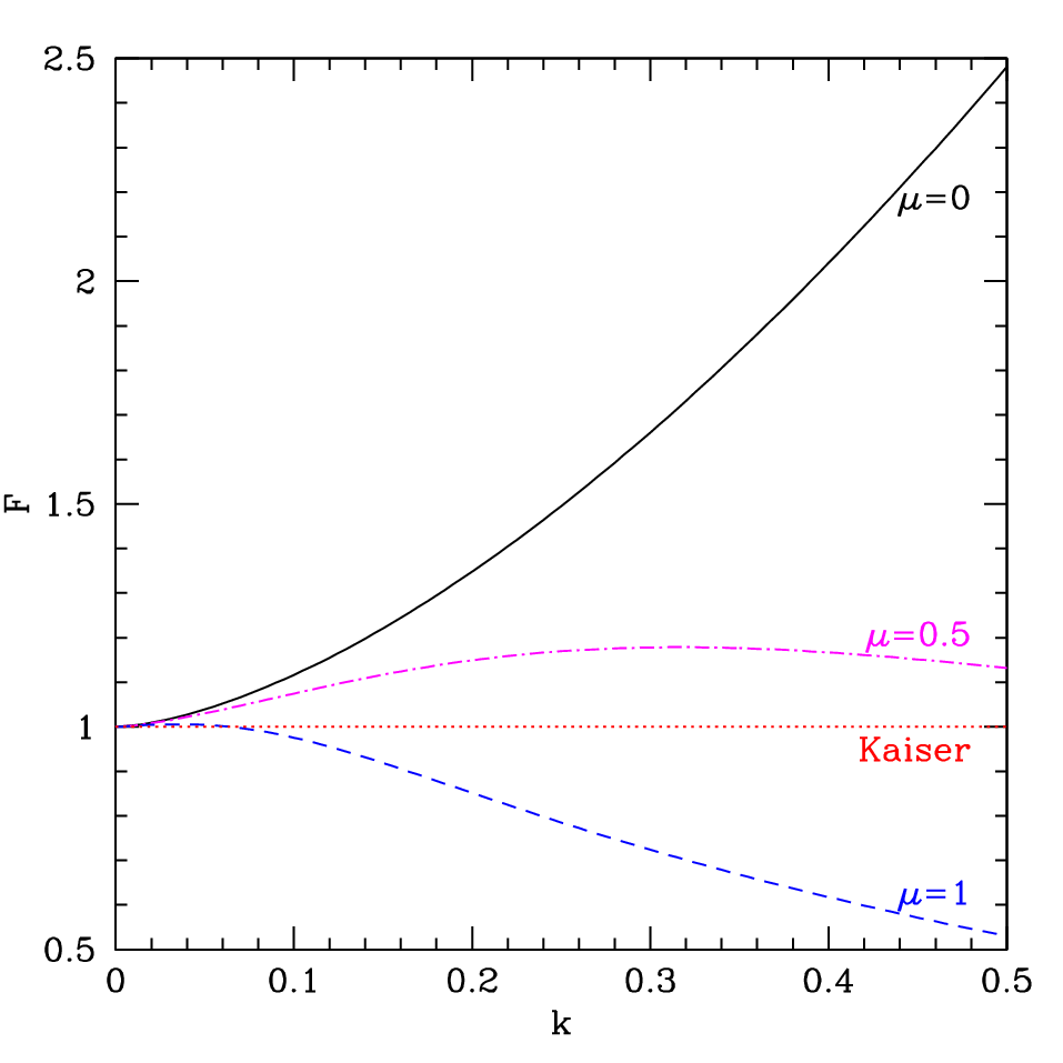
The resulting redshift space distortion reconstruction function of Eq. (3) is shown in Fig. 1. We emphasize that these are merely the fiducials; we allow the values of , , to float freely in bins of wavenumber. This provides a model independent variation of the power spectrum (within the reconstruction form) and we can then investigate the influence of such variations on the cosmological parameter estimation. Conversely, the question can be phrased as “what is the accuracy required on knowledge of the galaxy power spectrum in order to deduce the cosmology with confidence?”
We later contrast this fiducial with fiducial , i.e. assuming that perturbation theory (for example linear theory in the Kaiser case, although also works with higher order perturbation theory [6]) fully captures RSD effects in the model .
The analysis is carried out in the next sections in two ways: in Sec. III we compute the effect that a given level of unrecognized power spectrum deviation in some bin, i.e. a systematic error in modeling, has in biasing the cosmological conclusions, and in Sec. IV we recognize the existence of systematic uncertainties and treat them by marginalizing over the , , values for each bin.
II.3 Survey Characteristics and Parameters
For the galaxy redshift survey data we consider a next generation spectroscopic survey of the quality proposed for BigBOSS [19], covering 14000 deg2 from , with a galaxy number density of approximately . For the exact distribution adopted see Table 1. There are actually two populations of galaxies: luminous red galaxies (LRG) and emission line galaxies (ELG), each with their own galaxy bias value. These galaxy biases are taken as free parameters to be marginalized over, for each redshift bin of width . Their fiducials are with and , which provide good fits to observations. Galaxy populations with different biases can help reduce sample variance [20], with the Fisher matrix involving a sum over populations, i.e.
| (16) |
Note that for multiple populations the factor in Eq. (8) involves the shot noise, i.e. , of each population.
| 0.15 | 22.6 | 30.1 |
| 0.25 | 8.45 | 3.04 |
| 0.35 | 4.02 | 3.07 |
| 0.45 | 2.65 | 3.09 |
| 0.55 | 2.99 | 3.10 |
| 0.65 | 3.99 | 3.11 |
| 0.75 | 5.15 | 3.12 |
| 0.85 | 5.36 | 1.89 |
| 0.95 | 5.02 | 0.33 |
| 1.05 | 4.80 | 0.04 |
| 1.15 | 4.49 | – |
| 1.25 | 4.04 | – |
| 1.35 | 3.02 | – |
| 1.45 | 2.00 | – |
| 1.55 | 1.15 | – |
| 1.65 | 0.43 | – |
| 1.75 | 0.12 | – |
For the cosmological parameters we use the physical baryon density and physical cold dark matter density , reduced Hubble constant , scalar perturbation tilt and amplitude , dark energy equation of state parameters and , and gravitational growth index . The gravitational growth index gives an accurate description of the growth rate for both general relativity and a range of modified gravity models, and looking for deviations from its general relativistic value of acts as a test of gravity [21, 22]. The growth index is treated as an independent parameter (not a function of , ) and determines the growth factor at scale factor ,
| (17) |
that in this ansatz is used to convert the linear power spectrum delivered by CAMB at to another redshift , to account for the effects of modified gravitational growth. Note that the growth rate , and redshift space distortions were highlighted as a test of gravity in [23].
For the central question of RSD uncertainties we employ up to 12 free parameters, taking , , with independent values in each bin of width in wavenumber above /Mpc out to some . This corresponds to uncertainties . For the current work we follow [11, 12] and consider the uncertainties only as a function of wavenumber, not redshift, except in Sec. IV.3; we also take the KLL form to be accurate while allowing freedom in the parameters , , . In summary we fit for 8 cosmological parameters and up to 39 systematics parameters.
III Fisher Bias
The first question we are interested in answering is what is the sensitivity of the cosmological parameter determination to errors in modeling RSD. One might have or wrong, but if this does not mimic a change in cosmology then no harm is done. The Fisher bias formalism (see, e.g., [24, 25]) propagates misestimation of the observable or theoretical prediction, in this case the redshift space power spectrum, into biases on the fit parameters. Specifically, we consider the effect of errors in the bin values of , , .
The Fisher bias on a parameter from misestimating parameter is
| (18) |
where . The superscript “sub” denotes the Fisher submatrix without entries for the parameters whose misestimation we are studying. (For the specific case here, the submatrix will be for the cosmology and galaxy bias parameters, and the full matrix adds the reconstruction parameters one at a time. We later consider all the reconstruction parameters at once.) By evaluating the ratio for we can assess the sensitivity of the parameter estimation to the RSD modeling. To take a weak lensing example, [26] found that a particular form of matter power spectrum distortion with amplitude at high distorted estimation of derived from shear power spectrum measurement by a leverage factor of 18: a misestimation of 10% in yielded a bias in .
The bias can be compared to the statistical uncertainty on the parameter, either directly or through the risk statistic
| (19) |
Treating the bias as a systematic error in this way, to restrict the degradation in the statistical error to less than 20%, say, requires , thus putting a constraint on the allowable modeling error etc. We examine two, converse statistics: the cosmological degradation caused by a certain fractional misestimation of the reconstruction parameters , and the requirement on the reconstruction parameter to bound the cosmological parameter bias to less than a given factor of the statistical uncertainty, . These are respectively
| (20) | |||||
| (21) |
Figure 2, left panel, shows the matrix of degradations for fixed (i.e. 1% uncertainty on the reconstruction parameters), where the columns are the dark cosmological parameters and the rows are the reconstruction parameters. The right panel gives a similar matrix of the reconstruction requirements for fixed (which corresponds to ). One can scale the results for different fixed values according to the above equations. The stripe structure arises because the bias from , where the subscript indicates the center of the bin, is of opposite sign from that of , and lies in between near null effect, and similar for and .
The degradations in determination of the dark parameters , , are less than 22% for 1% shifts in the reconstruction parameters in all cases except , , and . For and the risk error on can exceed the statistical uncertainty by a factor 3. For the parameters the worst case is degradation by 1.5. These results offer indications of what physics must be most accurately understood, i.e. the nonlinearity from and, somewhat less critically, the velocity effects from .
In the converse analysis of what accuracy is required on the reconstruction parameters to ensure that a bias is restricted to below , we find that 5% accuracy is sufficient for all parameters except for the , plus and . Knowledge of and are needed to 0.3%, to 0.9%, to 1.4%, to 1.5%, and to 3.1%.

While these approaches give indications of sensitivity, they treat the cosmological parameters one by one while a power spectrum misestimation will generally impact several at once. This can either tighten or loosen overall requirements, depending on the covariances. To take this into account we use the method [27, 28]. This describes the fuller impact of biasing cosmology through quantifying how far from the fiducial the best fit cosmology is shifted relative to the confidence contour, taking into account degeneracies between the reconstruction and cosmological parameters. This measure is given by
| (22) |
where the sum runs only over the reduced parameter set whose bias we are interested in, e.g. and for a 2D – joint likelihood contour plot. The reduced Fisher matrix is marginalized over all other cosmological and galaxy bias parameters (the reconstruction parameters have already been taken into account in obtaining etc.). The bias accounts for the property that biases in, say, the direction of the narrow axis of the Fisher ellipse are more detrimental than those along the degeneracy direction.
Figure 3 illustrates the 2D bias induced in the dark energy and growth parameters, here for a 1% misestimation in the reconstruction parameters one by one. Most such reconstruction parameter errors do not significantly affect the joint parameter likelihood. In the – plane, none of the parameters and three of the parameters do not bias the best fit outside the contour, and remains within the contour. Only errors on the and parameters are particularly damaging, causing a bias of up to (approximately at the level). The covariance between the shifts in and is crucial; if the same bias in and an even larger bias in occurred such that the joint shift lay along the degeneracy axis, then the 2D bias would be scarcely outside the uncertainty contour. For the – plane, the biases are less severe, with only and causing more than a joint bias, at .
Treating the reconstruction errors one by one effectively takes a localized bump in the reconstruction function. A smooth variation would instead affect several of the reconstruction parameters at once; this has a different effect on the cosmological parameter bias. As an example, we simultaneously vary all four parameters by 1%. Since and have nearly opposite effects this reduces substantially the due to varying just one of them, e.g. from 39 to 7.7. The 2D bias due to such smooth variation is shown in the figures by the magenta squares.


While we have thus far been model independent in taking , , to be independent from one bin to the next, we can now consider the difference between two fiducial models for the overall reconstruction function . This then includes the effects of variations at all ’s simultaneously, and allows a study of bias as a function of . As we consider each successive bin at higher , we increase the number of modes, reducing the statistical uncertainty, but also often increase the deviation in the power spectra, increasing the bias in the cosmological parameters if we assume the wrong fiducial as the truth. The truth is taken to be as given by Eqs. (13)–(15) in Eq. (3), while the incorrect assumption is pure linear theory, i.e. simply the Kaiser form for redshift space distortions, equivalent to , .
This misestimation of the redshift space galaxy power spectrum causes a bias in cosmological parameters of
| (23) | |||||
The systematic biases tend to worsen with increasing , reaching in , in , and 0.2 in for /Mpc, and are much larger than the statistical uncertainties for all . This is not surprising since can deviate by a factor 2 from the KLL form. Thus, neglecting the uncertainties in the reconstruction parameters is not a viable option: we must take them into account.
IV Marginalization and Selfcalibration
As an alternative to requiring the power spectrum to subpercent accuracy and computing the bias from misestimated reconstruction parameters, we can fit for those parameters and calculate the increased uncertainty in cosmological parameters due to marginalization over the extra inputs. The basic question is how well the model needs to be known for precision determination of cosmology with RSD. This is similar to what [11, 12] did for matter power spectrum uncertainties applied to weak lensing cosmology. They used fractional power spectrum uncertainties in wavenumber bins, assumed constant with redshift, and applied some level of priors.
IV.1 Global Fit
Now our quantities , , in each wavenumber bin become fit parameters. Again, we can study the effects as we extend , using more bins and hence more parameters. Including these parameters means that we will not be biased any more with respect to the fiducial, but the enlarged parameter space will lead to some level of degradation of the statistical uncertainties, relative to fixing the reconstruction parameters, at the same .
Table 2 shows the effect of extending the data to higher , while simultaneously allowing for the additional reconstruction parameters in each bin. Despite the additional degrees of freedom in the fit, the cosmological parameter estimation sharpens with increasing . As long as the form of the reconstruction function holds, we obtain an accurate and unbiased cosmology even allowing for fitting variation in the amplitudes of , , in each bin. This is an extremely promising initial result for use of the reconstruction.
| Fiducial | 0.0226 | 0.112 | 0.7 | 0.96 | 2.47 | -0.99 | 0 | 0.55 | 0.275 |
|---|---|---|---|---|---|---|---|---|---|
| 0.00524 | 0.0189 | 0.0542 | 0.0524 | 0.538 | 0.599 | 2.23 | 0.177 | 0.0302 | |
| 0.00284 | 0.0102 | 0.0284 | 0.0288 | 0.325 | 0.197 | 0.779 | 0.0519 | 0.0159 | |
| 0.00219 | 0.00760 | 0.0219 | 0.0198 | 0.248 | 0.112 | 0.478 | 0.0272 | 0.0122 | |
| 0.00148 | 0.00508 | 0.0150 | 0.0130 | 0.170 | 0.0824 | 0.347 | 0.0193 | 0.00834 | |
| 0.00141 | 0.00478 | 0.0142 | 0.0119 | 0.158 | 0.0713 | 0.306 | 0.0163 | 0.00794 |
To better understand why the added fit parameters do not cause an overall degradation, we look at the correlation matrix of the 47 parameters in Fig. 4. The block of parameters 36–47, representing the reconstruction parameters, is not highly correlated with other parameters: correlation coefficients are below 0.58 (0.38 for parameters other than ). (Even within the block, only and , other than between the , have a correlation coefficient exceeding 0.8, reaching 0.90; this is expected since for a low expansion both and contribute as .) This means that the change in power spectrum shape due to adjusting the amplitudes of these parameters in is not degenerate with a change due to or other such parameters. That is, the influence of these parameters have different and dependences than those of cosmological parameters and so we find they can be separately fit.

Moreover, the reconstruction parameters are selfcalibrated by the data to good precision. All are determined to better than 3% (except , to 8%) and most to subpercent level. These propagate into determination of the power spectrum to the subpercent level for variation of each one individually by , except for the extreme cases of and () which gives 1.1% (1.2%) uncertainty. Most combinations, however, give subpercent precision. Adding all their uncertainties in the most unfavorable way generates an extreme of 2.6% power spectrum uncertainty. Thus unlike the weak lensing probe analyzed by [11, 12], redshift space distortions do not require any priors to be placed on the power spectrum parameters (assuming that the KLL reconstruction form is valid).
Remarkably, in addition to selfcalibration, the additional fit parameters have little impact on the cosmological parameter estimation, enlarging the uncertainties by only 9%, 22%, and 7% on , , and . And of course including the extra parameters removes any cosmology bias as suffered in the previous section (modulo model validity). Regarding the 12 extra reconstruction parameters, from Fig. 1 we see that is smooth in so taking bins of width 0.1 in is reasonable. For completeness, for bins of width 0.02 (and hence 60 extra parameters) we find that cosmological parameter estimation is mildly degraded, with uncertainties on , , increasing relative to 0.1 width by 16%, 33%, 17%.
IV.2 Maximum Wavenumber
Let us examine the dependence of the results on the maximum wavenumber used. Note that for the case, the cosmology parameters are not determined particularly well even though no reconstruction parameters are used for /Mpc. This is due to strong covariance with the 27 galaxy bias parameters. Once beyond the linear regime, this degeneracy is broken and the correlation coefficients drop, greatly improving the cosmological parameter determination (e.g. by factors of 2.9–3.4 on the dark parameters, for relative to ). This continues for higher , despite the addition of further reconstruction parameters, but gradually saturates. For example, while relative to the case the uncertainties on , , or at are greater by a factor , at the factor is 1.6, and at is 1.15, as seen in Fig. 5. Thus, having an accurate reconstruction form out to is sufficient for robust cosmological parameter estimation, while selfcalibration obviates the need for any prior knowledge of the values of the reconstruction parameters.

Binning such as we use is model independent and closest to the weak lensing work. This model independence is important since in the absence of a large suite of simulations we may have no particular confidence in parametrizations such as those in Eqs. (13-15). Recall that those equations merely give the fiducial values in each bin, and then we allow the bin values to float freely and marginalize over them. Given simulations we might be able to adopt specific forms and fit for a reduced set of parameters, e.g. the coefficients in those equations.
IV.3 Redshift Dependence
To give a first indication of whether adding redshift dependence to , , affects the conclusions we include a variation of the characteristic wavenumber scale entering in the nonlinearity amplitude in Eq. (13), i.e. the /Mpc, writing this as
| (24) |
and adding this evolution parameter to the fit. The simulation results in [15] indicate that relative to , the parameters and have negligible additional redshift dependence. Therefore we scale and by the same factor as , i.e.
| (25) | |||||
| (26) |
and the same for .
The introduction of redshift dependence through has little impact on the cosmological parameter estimation; the largest correlation coefficient of cosmologically is 0.31, with , and overall 0.83 with , while itself is determined to within 0.025. Figure 6 shows the influence on dark cosmology parameter estimation of marginalization over the reconstruction parameters with and without redshift dependence, and fixing the reconstruction parameters (i.e. with a total of 48, 47, or 35 parameters). Uncertainties on , , and increase by only 0.8%, 0.2%, 5% respectively upon including . Other forms of redshift dependence may have different cosmological impact, and this deserves further analysis through simulations, but the scaling of the characteristic wavenumber as used here should give a reasonable first indication.


IV.4 Nonlinear Power Spectrum
The greatest effect of uncertainty in the reconstruction function comes from the parameters , as seen in Fig. 1 and in Sec. III regarding the parameter bias. Recall that arises from the nonlinear effects in the density field, and even exists when . In this limit acts to map the linear real space density power spectrum to the nonlinear regime. Therefore, if we had a robust nonlinear (or quasilinear) real space power spectrum then we would have no need of a separate parameter as then (this has been tested and found accurate to subpercent level by [15]). Substantial effort is going into developing cosmic emulators [29] that could provide accurate nonlinear power spectra, eventually including the full set of cosmological parameters and redshifts considered here. Since that is still in the future, we consider the nonlinear prescription of Halofit [30] to get an indication of the potential impact on our conclusions.
The linear power spectrum at a given redshift is fed into Halofit to give the approximate nonlinear form. This removes the need for , setting this equal to one for all and . As indicated earlier in this section, the simulation results from [15] imply that for such a normalized then the quantities and become substantially redshift independent. Therefore we do not need any hypothetical model such as the parametrization, making the entire analysis more robust. Furthermore, Halofit includes cosmology dependence and so no assumption about universality of is needed.
We show the results for cosmological parameter estimation in Table 3, for /Mpc, for the three cases of using the model independent approach of fitting for in bins, using Halofit and , and using the revised version of Halofit from [31] and . In all cases we still fit for the binned values of and . The use of functional forms for the nonlinear real space power spectrum allows better determination of the cosmological parameters, by 12%, 28%, 12% for , , respectively (15%, 33%, 15% for revised Halofit, which has slightly more quasilinear power). This offers some promise for the future use of cosmic emulators, but in this paper we prefer to be conservative in the estimations and use the model independent approach.
| Fit | 0.0713 | 0.306 | 0.0163 | 0.00794 |
|---|---|---|---|---|
| Halofit | 0.0624 | 0.220 | 0.0143 | 0.00678 |
| New Halofit | 0.0603 | 0.206 | 0.0139 | 0.00608 |
V Conclusions
With the ability to map galaxy clustering in three dimensions over large volumes of the universe comes the necessity for accurate theoretical interpretation. This entails linking the isotropic, linear theory real space density power spectrum to the observed anisotropic, nonlinear redshift space galaxy power spectrum. We have investigated here some of the relevant issues involving nonlinearities in the density field and velocity effects, using the Kwan-Lewis-Linder analytic redshift space reconstruction function calibrated from numerical simulations.
The main question addressed is to what accuracy the anisotropic redshift space power spectrum must be known in order to achieve robust cosmological conclusions. We propagate uncertainties in the power spectrum through a model independent binning of reconstruction amplitudes with wavenumber and assess the effects of deviations from fiducial values. To avoid biasing cosmological parameters such as the dark energy equation of state and gravitational growth index requires down to 0.3% accuracy on the reconstruction parameters in the most stringent cases, while smoother deviations give more tractable requirements. Note that it is only those deviations that mimic cosmological variations that are most important.
A more flexible and robust approach is to carry out a global fit for the binned reconstruction parameters simultaneously with the cosmological parameters, which avoids biasing the results so long as the form of the KLL function is a good approximation. With 8 cosmology parameters and 39 systematics parameters we find that a next generation galaxy redshift survey such as BigBOSS can tightly and accurately constrain cosmology, for example determining the equation of state time variation to 0.3 and testing gravity through the growth index to 3%. No external priors on the reconstruction parameters are necessary as they are selfcalibrated by the survey, most at the subpercent level. This also corresponds to subpercent calibration of the redshift space power spectrum.
We have tested the robustness of the conclusions by adding redshift evolution, which has little effect, varying the number of wavenumber bins, and exploring the leverage from increasing the maximum wavenumber used, . Cosmological leverage plateaus by /Mpc so the KLL form need only apply up to this scale. We made no assumptions about the departure from linearity, allowing the nonlinearity amplitude to float in a model independent manner in bins of , but also then analyzed the impact of adopting a nonlinear prescription such as Halofit (or its revision). This improved the cosmology estimation and offers a promising sign to motivate continued development of cosmic emulators for the nonlinear power spectrum.
Several areas exist for further development. The KLL form has been tested for dark matter, but [15] indicates it is successful for halos as well. Eventually this must be extended to galaxies, a major undertaking. On the positive side, we achieved excellent results using reconstruction starting from simple linear theory (Kaiser approximation); higher order perturbation theory approaches extend the range where reconstruction is milder. Universality, i.e. cosmology dependence, of the reconstruction is a major topic for future investigation, requiring large suites of cosmological simulations, again suited for emulators. We have taken a first step toward addressing this effect by exploring the influence of using Halofit and new Halofit cosmological dependences for the nonlinearity. Simulations may also enable us to compress the information in bins down to a smaller set of parameters.
Redshift space distortions provide a powerful tool for measuring the growth rate of cosmic structure, and delivering insights on the competition between the gravitational laws driving clustering and accelerated expansion suppressing it. The results here give encouraging indications, and quantitative measures, that theoretical analysis can take into account robustly the nonlinear and velocity effects to extract accurate cosmology from the forthcoming large volume redshift surveys.
Acknowledgements.
We thank Sudeep Das, Juliana Kwan, and Alberto Vallinotto for helpful discussions. This work has been supported by DOE grant DE-SC-0007867 and the Director, Office of Science, Office of High Energy Physics, of the U.S. Department of Energy under Contract No. DE-AC02-05CH11231. EL acknowledges World Class University grant R32-2009-000-10130-0 through the National Research Foundation, Ministry of Education, Science and Technology of Korea; JS is supported by the Dark Cosmology Centre, funded by the Danish National Research Foundation, and thanks LBNL for additional support.References
- [1] W.J. Percival & M. White, MNRAS 393, 297 (2009) [arXiv:0808.0003]
- [2] T. Okumura & Y.P. Jing, ApJ 726, 5 (2011) [arXiv:1004.3548]
- [3] E. Jennings, C.M. Baugh, S. Pascoli, MNRAS 410, 2081 (2011) [arXiv:1003.4282]
- [4] E. Jennings, C.M. Baugh, S. Pascoli, ApJL 727, 9 (2011) [arXiv:1011.2842]
- [5] J. Tang, I. Kayo, M. Takada, MNRAS 416, 2291 (2011) [arXiv:1103.3614]
- [6] J. Kwan, G.F. Lewis, E.V. Linder, ApJ 748, 78 (2012) [arXiv:1105.1194]
- [7] R. Scoccimarro, Phys. Rev. D 70, 083007 (2004) [arXiv:astro-ph/0407214]
- [8] A. Taruya, T. Nishimichi, S. Saito, Phys. Rev. D 82, 063522 (2010) [arXiv:1006.0699]
- [9] B.A. Reid & M. White, MNRAS 417, 1913 (2011) [arXiv:1105.4165]
- [10] T. Okumura, U. Seljak, P. McDonald, V. Desjacques, JCAP 1202, 010 (2012) [arXiv:1109.1609]
- [11] D. Huterer & M. Takada, Astropart. Phys. 23, 369 (2005) [arXiv:astro-ph/0412142]
- [12] A.P. Hearin, A.R. Zentner, Z. Ma, JCAP 1204, 034 (2012) [arXiv:1111.0052]
- [13] A. Lewis, A. Challinor, A. Lasenby, ApJ 538, 473 (2000) [arXiv:astro-ph/9911177]; http://camb.info
- [14] N. Kaiser, MNRAS 227, 1 (1987)
- [15] J. Kwan, Ph.D. thesis, University of Sydney (2011)
- [16] H.A. Feldman, N. Kaiser, J.A. Peacock, ApJ 426, 23 (1994) [arXiv:astro-ph/9304022]
- [17] H-J. Seo & D.J. Eisenstein, ApJ 598, 720 (2003) [arXiv:astro-ph/0307460]
- [18] A. Stril, R.N. Cahn, E.V. Linder, MNRAS 404, 239 (2010) [arXiv:0910.1833]
- [19] D. Schlegel et al, arXiv:1106.1706 ; http://bigboss.lbl.gov
- [20] P. McDonald & U. Seljak, JCAP 0910, 007 (2009) [arXiv:0810.0323]
- [21] E.V. Linder, Phys. Rev. D 72, 043529 (2005) [arXiv:astro-ph/0507263]
- [22] E.V. Linder & R.N. Cahn, Astropart. Phys. 28, 481 (2007) [arXiv:astro-ph/0701317]
- [23] E.V. Linder, Astropart. Phys. 29, 336 (2008) [arXiv:0709.1113]
- [24] L. Knox, R. Scoccimarro, S. Dodelson, Phys. Rev. Lett. 81, 2004 (1998) [arXiv:astro-ph/9805012]
- [25] E.V. Linder, Astropart. Phys. 26, 102 (2006) [arXiv:astro-ph/0604280]
- [26] S. Das, R. de Putter, E.V. Linder, R. Nakajima, JCAP 1211, 011 (2012) [arXiv:1102.5090]
- [27] S. Dodelson, C. Shapiro, M. White, Phys. Rev. D 73, 023009 (2006) [arXiv:astro-ph/0508296]
- [28] C. Shapiro, ApJ 696, 775 (2009) [arXiv:0812.0769]
- [29] E. Lawrence, K. Heitmann, M. White, D. Higdon, C. Wagner, S. Habib, B. Williams, ApJ 713, 1322 (2010) [arXiv:0912.4490] ; http://www.lanl.gov/projects/cosmology/CosmicEmu
- [30] R.E. Smith et al, MNRAS 341, 1311 (2003) [arXiv:astro-ph/0207664]
- [31] R. Takahashi, M. Sato, T. Nishimichi, A. Taruya, M. Oguri, arXiv:1208.2701