Reply to Comment on “Towards a large deviation theory for strongly correlated systems”

Before addressing in detail the Comment by Touchette [1] on our paper [2], let us describe the physical scenario within which we have undertaken a possible generalization of the standard large deviation theory (LDT). A standard many-body Hamiltonian system in thermal equilibrium with a ther- mostat at temperature $T$ is described by the Boltzmann-Gibbs (BG) weight, proportional to $e^{-\beta{\cal H}_{N}}=e^{-\beta[{\cal H}_{N}/N]N}$, where ${\cal H}_{N}$ is the $N$-particle Hamiltonian, and $\beta\equiv 1/k_{B}T$. For standard Hamiltonian systems (typically involving short-range interactions and an ergodic behavior), the total energy is extensive. Consequently, the quantity $[{\cal H}_{N}/N]$ scales with $N$, analogously to a (thermodynamically) intensive variable. This is to be compared with the LDT probability $P(N)\sim e^{-r_{1}N}$, where the rate function $r_{1}$ (the meaning of the subindex $1$ will soon become clear) is related to a BG entropic quantity per particle, and plays a role analogous to $\beta[\cal{H}_{N}/N]$ (we remind that, for such standard systems, $\beta$ is an intensive variable).

If now we focus on say a $d$-dimensional classical system involving two- body interactions whose potential asymptotically decays at long distance $r$ like $-A/r^{\alpha}$ $(A>0;\alpha\geq 0)$, the canonical BG partition function converges whenever the potential is integrable, i.e. for $\alpha/d>1$ (short-range interactions), and diverges whenever it is nonintegrable, i.e. for $0\leq\alpha/d\leq 1$ (long-range interactions). The use of the BG weight becomes unjustified [“illusory” in Gibbs words [3] for say Newtonian gravitation, which in the present notation corresponds to $(\alpha,d)=(1,3)$, hence $\alpha/d=1/3$] in the later case because of the divergence of the BG partition function. We might therefore expect the emergence of some function $f({\cal H}_{N})$ different from the exponential one, in order to describe some specific stationary (or quasi-stationary) states differing from thermal equilibrium. The Hamiltonian ${\cal H}_{N}$ generically scales like $N{\tilde{N}}$ with ${\tilde{N}}\equiv\frac{N^{1-\alpha/d}-1}{1-\alpha/d}\equiv\ln_{\alpha/d}N$ (with the $q$-logarithmic function defined as $\ln_{q}z\equiv\frac{z^{1-q}-1}{1-q};\,z>0;\,\ln_{1}z=\ln z$). Notice that ($N\to\infty$) ${\tilde{N}}\sim N^{1-\alpha/d}/(1-\alpha/d)$ for $1\leq\alpha/d<1$, ${\tilde{N}}\sim\ln N$ for $\alpha/d=1$, and ${\tilde{N}}\sim 1/(\alpha/d-1)$ for $\alpha/d>1$. The particular case $\alpha=0$ yields ${\tilde{N}}\sim N$, thus recovering the usual prefactor of Mean Field theories. The quantity $\beta{\cal H}_{N}$ can be rewritten as $[(\beta{\tilde{N}}){\cal H_{N}}/(N{\tilde{N}})]N=[{\tilde{\beta}}{\cal H}_{N}/(N{\tilde{N}})]N$, where ${\tilde{\beta}}\equiv\beta{\tilde{N}}\equiv 1/k_{B}{\tilde{T}}={\tilde{N}}/k_{B}T$ plays the role of an intensive variable. The correctness of all these scalings has been profusely verified in various kinds of thermal [4], diffusive [5] and geometrical (percolation) [6] systems (see also [7, 8]). We see that, not only for the usual case of short-range interactions but also for long-range ones, $[{\tilde{\beta}}{\cal H}_{N}/(N{\tilde{N}})]$ plays a role analogous to an intensive variable. The $q$-exponential function $e_{q}^{z}\equiv[1+(1-q)z]^{\frac{1}{1-q}}$ ($e_{1}^{z}=e^{z}$) (and its associated $q$-Gaussian [9]) has already emerged, in a considerable amount of nonextensive and similar systems (see [10, 11, 12, 13, 14, 15, 16, 17, 18, 19, 20, 21, 22, 23, 24, 25, 26, 27, 28, 29, 30, 31] among others), as the appropriate generalization of the exponential one (and its associated Gaussian). Therefore, it appears as rather natural to conjecture that, in some sense that remains to be precisely defined, the LDT expression $e^{-r_{1}N}$ becomes generalized into something close to $e_{q}^{-r_{q}N}$ ($q\in{\cal R}$), where the generalized function rate $r_{q}$ should be some generalized entropic quantity per particle. Let us stress a crucial point: we are not proposing for long-range interactions, and other nonstandard systems, something like $e_{q}^{-r_{q}N^{\gamma}}$ with $\gamma\neq 1$, but we are expecting instead $\gamma=1$, i.e., the extensivity of the total $q$-generalized entropic form to still hold [32], in order to be consistent with many other related results (e.g., [8, 33, 34, 35]). We shall soon see that this important assumption indeed appears to be verified in the model, characterized by $(Q,\gamma,\delta)$ , that we numerically studied in [2].

Let us start by exhibiting that its $N\to\infty$ LDT asymptotic behavior numerically satisfies

with $\eta\equiv\frac{1}{q-1}=\frac{\gamma(3-Q)}{Q-1}>0$ [2]. This implies the existence of a generically positive finite $B(x)$ such that

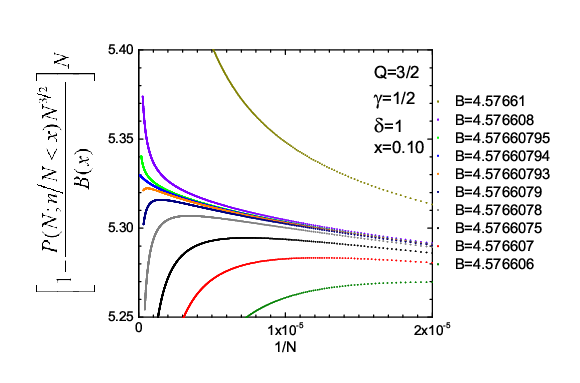
$C(x)$ being a generically positive finite number for all values of $x$ different from 1/2. This is indeed verified, as exhibited in Fig. 1 and 2. More precisely, we verify for fixed $(Q,\gamma,\delta)$ that $B(x)$ is unique for any given $x$, whereas $C(x)$ is in fact a set of values, noted $\{C_{j}(x)\}$, with $j=1,2,\dots,j_{max}$ (the value of $j_{max}$ depends on $x$; for example, we can see that, for the illustration exhibited in Fig. 2, $j_{max}=10$ for $x=0.1$). Let us emphasize that the $1/N$ correction to the power law $1/N^{\eta}$ in (1) is consistent with the total entropy of the system always being extensive in the thermodynamical sense.

Let us next check the conjecture made in [2], namely that $P(N;n/N<x)$ is, for $q>1$, well approached by

By identifying this expansion with Eq. (1) we obtain

and

Since $B(x)$ and $\{C_{j}(x)\}$ are numerically known, we can easily calculate $\{a_{j}(x)\}$ and $\{r_{q}^{(j)}(x)\}$ by using Eqs. (4) and (5). Knowing these, we calculate $a_{j}(x)\,e_{q}^{-r_{q}^{(j)}(x)N}$ ($j=1,2,\dots,j_{max}$) and compare with our numerical data. We then bound our numerical results from both below and above (see Figs. 3 and 4 for illustrations). More precisely, for each value of $x$, we have adopted two values, noted $C_{lower\,bound}(x)$ and $C_{upper\,bound}(x)$, such that $q$-exponential upper and lower bounds for the entire set of numerical values for $P(N;n/N<x)$ are obtained. These $C_{lower\,bound}(x)$ and $C_{upper\,bound}(x)$ values turn out to be comparable to the corresponding set $\{C_{j}(x)\}$ (see Fig. 2). In other words, we obtain the values of $C_{lower\,bound}(x)$, $C_{upper\,bound}(x)$, $r_{q}^{(upper\,bound)}(x)$ and $r_{q}^{(lower\,bound)}(x)$, consistent with Eq. (5). By introducing these values in Eq. (4) we obtain $a_{q}^{(upper\,bound)}(x)$ and $a_{q}^{(lower\,bound)}(x)$, and verify that, in the model studied in [2], $\forall x$, $\forall N$,

We may summarize the above considerations by conjecturing that, for all strongly correlated systems which have $Q$-Gaussians ($Q>1$) as attractors in the sense of the central limit theorem (see [33]), a model-dependent set $[q>1,B(x)>0,r_{q}^{(lower\,bound)}(x)>0,r_{q}^{(upper\,bound)}(x)>0]$ might exist such that $P(N;n/N<x)$ generically satisfies inequalities (6). In our present example, this set depends on $(Q,\gamma,\delta)$. Typical values of $[r_{q}^{(lower\,bound)}(x),r_{q}^{(upper\,bound)}(x)]$ are illustrated in Fig. 5 and compared with $q$-generalized entropic quantities.

Touchette mentions Kaniadakis’ $\kappa$-logarithm and $\kappa$-exponential [36] as an alternative to the $q$-exponential and $q$-logarithm herein conjectured. Let us address this point through the definition

(Notice a misprint in the definition of the $\kappa$-logarithm appearing in Touchette’s Comment). It straightforwardly follows the asymptotic series

The dominant term is a power-law, and at this approximation it is trivially as admissible as virtually any other power-law. However, we verify a highly meaningful discrepancy with the $q$-exponential function, namely that its subdominant correction is in $1/N^{2}$, instead of $1/N$. This fact excludes the $\kappa$-exponential function as an adequate one for the present purpose; indeed, it cannot satisfactorily reproduce the results exhibited in Figs. 3 and 4 .

A point remains to be discussed. The Lévy-Gnedenko theorem concerns sums of infinitely many independent (or nearly independent, in a specific sense) random variables, whereas the 2008 $Q$-central limit theorem [33] concerns sums of infinitely many strongly correlated variables within a specific class. The first case corresponds to divergent standard variance, whereas the second one concerns finite ${\bar{Q}}$-variance (${\bar{Q}}=2Q-1$; see details in [33]). The attractors for the former case are Lévy distributions, whereas those for the latter are $Q$-Gaussians. Both classes have long tails. For the Lévy distributions, the decay is slower than $1/|x|^{3}$ and faster than $1/|x|$; for the $q$-Gaussians, any power-law faster than $1/|x|$ is admissible. It is known that they have this and other relevant differences. They always differ excepting for an unique case, which happens to be precisely the case focused on by Touchette, i.e. $Q=2$, namely the Cauchy-Lorentz distribution (named after Cauchy by mathematicians, and after Lorentz by physicists). They can be simply thought as having $r_{1}(x)=0$, which, as acknowledged by Touchette, is not particularly enlightening. But they can be also thought in a much more interesting way, namely as having $r_{2}(x)$ different from zero, which neatly illustrates the usefulness of the approach adopted in [2]. In fact, it is well known that $Q=2$ is a highly peculiar case within the interval $1<Q<3$. For example, the anomalous diffusion coefficient in the nonlinear Fokker-Planck equation known as the Porous Medium Equation and discussed in [18] changes its sign precisely at $Q=2$ (see also [19]). The fact that, for $Q=2$, $r_{1}=0$ whereas $r_{q}\neq 0$ is totally analogous to a variety of dissipative one-dimensional maps whose Lyapunov exponent vanishes at the edge of chaos. In such cases, the use of the nonadditive entropy $S_{q}$ instead of the BG one makes the discussion much richer since it enables a simple quantitative characterization of the nonlinear dynamical behavior (by generalizing the standard exponential sensitivity to the initial conditions when the maximal Lyapunov exponent is strictly positive to the $q$-exponential form at the edge of chaos, when the maximal Lyapunov exponent vanishes). This has been verified both analytically and numerically in very many cases [12].

Let us conclude by saying that point (i) of the present Abstract is agreeably discussed in Touchette’s Comment, but a neat analysis of the important points (ii) and (iii) is notoriously absent in his paper. In other words, the $q$-exponential ansatz proposed in [2] for (asymptotically) generalizing the standard LDT remains (either exactly or approximatively: see the quantity (2), expected to be finite, and the inequalities (6)) as a very strong candidate for a wide class of systems whose elements are strongly correlated. This fact may be seen as a strong indication that, consistently with other results available in the literature (see [4, 5, 6, 8, 14, 32]), the total entropy remains extensive (i.e., thermodynamically admissible) even in nonstandard cases where the BG entropy fails to be extensive. Any analytical results along these or similar lines would obviously be highly interesting and welcome.

References

- [1] H. Touchette, Comment on “Towards a large deviation theory for strongly correlated systems” (2012).
- [2] G. Ruiz and C. Tsallis, Phys. Lett. A 376, 2451 (2012).
- [3] J.W. Gibbs, Elementary Principles in Statistical Mechanics – Developed with Especial Reference to the Rational Foundation of Thermodynamics, C. Scribner’s Sons, New York, 1902; Yale University Press, New Haven, 1948; OX Bow Press, Woodbridge, Connecticut, 1981 (page 35).
- [4] P. Jund, S.G. Kim and C. Tsallis, Phys. Rev. B 52, 50 (1995); J.R. Grigera, Phys. Lett. A 217, 47 (1996); S.A. Cannas and F.A. Tamarit, Phys. Rev. B 54, R12661 (1996); L.C. Sampaio, M.P. de Albuquerque and F.S. de Menezes, Phys. Rev. B 55, 5611 (1997); C. Anteneodo and C. Tsallis, Phys. Rev. Lett. 80, 5313 (1998); Curilef and C. Tsallis, Phys. Lett. A 264, 270 (1999); R.F.S. Andrade and S.T.R. Pinho, Phys. Rev. E 71, 026126 (2005).
- [5] C.A. Condat, J. Rangel and P.W. Lamberti, Phys. Rev. E 65, 026138 (2002).
- [6] H.H.A. Rego, L.S. Lucena, L.R. da Silva and C. Tsallis, Physica A 266, 42 (1999); U.L. Fulco, L.R. da Silva, F.D. Nobre, H.H.A. Rego and L.S. Lucena, Phys. Lett. A 312, 331 (2003).
- [7] C. Tsallis, J. Stat. Phys. 52, 479 (1988).
- [8] C. Tsallis, Introduction to Nonextensive Statistical Mechanics - Approaching a Complex World (Springer, New York, 2009).
- [9] Let us remind that the -Gaussians for are also called -distributions in the plasma physics community, and also occasionally generalized Lorentzians; for special rational values of they correspond to the Student’s -distributions for an integer number of degrees of freedom. For special rational values of , -Gaussians correspond to the -distributions (which have a compact support).
- [10] F.A. Tamarit, S.A. Cannas and C. Tsallis, Eur. Phys. J. B 1, 545 (1998).
- [11] C. Anteneodo and C. Tsallis, J. Mol. Liq. 71, 255 (1997).
- [12] U. Tirnakli, C. Tsallis and M.L. Lyra, Eur. Phys. J. B 11, 309 (1999); F. Baldovin and A. Robledo, Europhys. Lett. 60, 518 (2002); F. Baldovin and A. Robledo, Phys. Rev. E 66, R045104 (2002); E.P. Borges, C. Tsallis, G.F.J. Ananos and P.M.C. Oliveira, Phys. Rev. Lett. 89, 254103 (2002); F. Baldovin and A. Robledo, Phys. Rev. E 69, 045202(R) (2004); E. Mayoral and A. Robledo, Physica A 340, 219 (2004); G.F.J. Ananos and C. Tsallis, Phys. Rev. Lett. 93, 020601 (2004). G. Casati, C. Tsallis and F. Baldovin, Europhys. Lett. 72, 355 (2005); E. Mayoral and A. Robledo, Phys. Rev. E 72, 026209 (2005); G. Ruiz and C. Tsallis, Eur. Phys. J. B 67, 577 (2009).
- [13] C. Tsallis, J.C. Anjos and E.P. Borges, Phys. Lett. A 310, 372 (2003).
- [14] M. Gell-Mann and C. Tsallis, Nonextensive Entropy - Interdisciplinary Applications (Oxford University Press, New York, 2004).
- [15] A. Rodriguez, V. Schwammle and C. Tsallis, JSTAT P09006 (2008); R. Hanel, S. Thurner and C. Tsallis, Eur. Phys. J. B 72, 263 (2009); A. Rodriguez, C. Tsallis, J. Math. Phys. 51, 073301 (2010).
- [16] J. S. Andrade Jr., G.F.T. da Silva, A.A. Moreira, F.D. Nobre and E.M.F. Curado, Phys. Rev. Lett. 105, 260601 (2010); Y. Levin and R. Pakter, Phys. Rev. Lett. 107, 088901 (2011); J. S. Andrade Jr., G.F.T. da Silva, A.A. Moreira, F.D. Nobre and E.M.F. Curado, Phys. Rev. Lett. 107, 088902 (2011); M.S. Ribeiro, F.D. Nobre and E.M.F. Curado, in Special Issue Tsallis Entropy, ed. A. Anastasiadis, Entropy 13, 1928 (2011); M.S. Ribeiro, F.D. Nobre and E.M.F. Curado, Phys. Rev. E 85, 021146 (2012); M.S. Ribeiro, F.D. Nobre and E.M.F. Curado, Overdamped motion of interacting particles in general confining potentials: Time-dependent and stationary-state analyses, Eur. Phys. J. B (2012), in press.
- [17] U. Tirnakli, H.J. Jensen and C. Tsallis, EPL 96, 40008 (2011).
- [18] A.R. Plastino and A. Plastino, Physica A 222, 347 (1995); C. Tsallis and D.J. Bukman, Phys. Rev. E 54, R2197 (1996); L.C. Malacarne, R.S. Mendes, I.T. Pedron and E.K. Lenzi, Phys. Rev. E 65, 052101 (2002).
- [19] I.T. Pedron, R.S. Mendes, T.J. Buratta, L.C. Malacarne and E.K. Lenzi, Phys. Rev. E 72, 031106 (2005).
- [20] L. Borland, Phys. Lett. A 245, 67 (1998); L. Borland, F. Pennini, A. R. Plastino and A. Plastino Eur. Phys. J. B 12, 285 (1999); C. Anteneodo and C. Tsallis, J. Math. Phys. 44, 5194 (2003); V. Schwammle, E.M.F. Curado and F.D. Nobre, Eur. Phys. J. B 58, 159-165 (2007); V. Schwammle, F.D. Nobre and E.M.F. Curado, Phys. Rev. E 76, 041123 (2007); M.A. Fuentes and M.O. Caceres, Phys. Lett. A 372, 1236 (2008) [to compare with the present paper, it must be done ]; B.C.C. dos Santos and C. Tsallis, Phys. Rev. E 82, 061119 (2010); A. Mariz and C. Tsallis, Phys. Lett. A 376, 3088 (2012).
- [21] A. Pluchino, A. Rapisarda and C. Tsallis, EPL 80, 26002 (2007); A. Pluchino, A. Rapisarda and C. Tsallis, Physica A 387, 3121 (2008).
- [22] C. Anteneodo and C. Tsallis, Phys. Rev. Lett. 80, 5313 (1998).
- [23] A. Upadhyaya, J.-P. Rieu, J.A. Glazier and Y. Sawada, Physica A 293, 549 (2001).
- [24] S. Thurner, N. Wick, R. Hanel, R. Sedivy and L.A. Huber, Physica A 320, 475 (2003).
- [25] K.E. Daniels, C. Beck and E. Bodenschatz, Physica D 193, 208 (2004).
- [26] L.F. Burlaga and A.F.Vinas, Physica A 356, 375 (2005); L.F. Burlaga, A.F. Vinas, N.F. Ness and M.H. Acuna, Astrophys. J. 644, L83 (2006); L.F. Burlaga and N.F. Ness, Astrophys. J. 703, 311 (2009); L.F. Burlaga, N.F. Ness, M.H. Acuna, Astrophys. J. 691, L82 (2009); J. Cho, A. Lazarian, Astrophys. J. 701, 236 (2009); L.F. Burlaga and N.F. Ness, Astrophys. J. 725, 1306 (2010) 1306; A. Esquivel, A. Lazarian, Astrophys. J. 710, 125 (2010); L.F. Burlaga and N.F. Ness, Astrophys. J. 737, 35 (2011).
- [27] P. Douglas, S. Bergamini and F. Renzoni, Phys. Rev. Lett. 96, 110601 (2006).
- [28] B. Liu and J. Goree, Phys. Rev. Lett. 100, 055003 (2008); R.M. Pickup, R. Cywinski, C. Pappas, B. Farago, P. Fouquet, Phys. Rev. Lett. 102, 097202 (2009); R.G. DeVoe, Phys. Rev. Lett. 102, 063001 (2009).
- [29] CMS Collaboration, J. High Energy Phys. 02, 041 (2010); CMS Collaboration, Phys. Rev. Lett. 105, 022002 (2010); CMS Collaboration, J. High Energy Phys. 09, 091 (2010); CMS Collaboration, J. High Energy Phys. 08, 086 (2011); CMS Collaboration, J. High Energy Phys. 05, 064 (2011); ALICE Collaboration, Phys. Lett. B 693, 53 (2010); ALICE Collaboration, Eur. Phys. J. C 71, 1594 (2011); ALICE Collaboration, Eur. Phys. J. C 71, 1655 (2011); ATLAS Collaboration, New J. Physics 13, 053033 (2011); PHENIX Collaboration, Phys. Rev. D 83, 052004 (2011); PHENIX Collaboration, Phys. Rev. C 83, 024909 (2011); PHENIX Collaboration, Phys. Rev. C 83, 064903 (2011); PHENIX Collaboration, Phys. Rev. C 84, 044902 (2011); M. Shao, L. Yi, Z.B. Tang, H.F. Chen, C. Li, Z.B. Xu, J. Phys. G 37, 084104 (2010); A. Tawfik, Nuclear Phys. A 859, 63 (2011).
- [30] U. Tirnakli, C. Beck and C. Tsallis, Phys. Rev. E 75, 040106(R) (2007); U. Tirnakli, C. Tsallis and C. Beck, Phys. Rev. E 79, 056209 (2009); C. Tsallis and U. Tirnakli, J. Phys. Conf. Series 201, 012001 (2010).
- [31] F.D. Nobre, M.A. Rego-Monteiro and C. Tsallis, Phys. Rev. Lett. 106, 140601 (2011); F.D. Nobre, M.A. Rego-Monteiro and C. Tsallis, EPL 97, 41001 (2012).
- [32] C. Tsallis, M. Gell-Mann and Y. Sato, Proc. Nat. Acad. Sci. 102, 15377 (2005); F. Caruso and C. Tsallis, Phys. Rev. E 78, 021101 (2008);A . Saguia and M.S. Sarandy, Phys. Lett. A 374, 3384 (2010).
- [33] S. Umarov, C. Tsallis and S. Steinberg, Milan J. Math. 76, 307 (2008); for a simplified version, see S.M.D. Queiros and C. Tsallis, AIP Conference Proceedings 965, 21 (New York, 2007). See also S. Umarov, C. Tsallis, M. Gell-Mann and S. Steinberg, J. Math. Phys. 51, 033502 (2010).
- [34] C. Vignat and A. Plastino, J. Phys. A 40, F969 (2007); M. Przystalski, Phys. Lett. A 374, 123 (2009); M.G. Hahn, X.X. Jiang and S. Umarov, J. Phys. A 43, 165208 (2010).
- [35] A gap has been recently detected, by H.J. Hilhorst, J. Stat. Mech., P10023 (2010), in the proofs of [33], namely that the -Fourier transform has not, for , an inverse in the simple sense that the standard Fourier transform has. This point certainly is interesting on its own, even if the thesis of the theorems are consistent with alternative proofs that do not use the -Fourier transform. Very recently it has been shown by M. Jauregui and C. Tsallis, Phys. Lett. A 375, 2085 (2011), M. Jauregui, C. Tsallis and E.M.F. Curado, J. Stat. Mech., P10016 (2011), A. Plastino and M.C. Rocca, Physica A 391, 4740 (2012), and A. Plastino and M.C. Rocca, Milan J. Math. (2012), DOI 10.1007/s00032-012-0179-6, that an unique inverse of the -Fourier transform does exist if some supplementary information is given (something which is unnecessary only for ). The use of these results in order to fill the mentioned gap in the proofs of the theorems [33] remains now to be done.
- [36] G. Kaniadakis, Physica A 296, 405 (2001).