1Introduction

ANL-HEP-PR-12-84

Higgs CP Properties From Early LHC Data

A. Freitas¹, P. Schwaller^2,3

¹ Pittsburgh Particle physics, Astrophysics & Cosmology Center (PITT-PACC), Department of Physics & Astronomy, University of Pittsburgh, Pittsburgh, PA 15260, USA

² HEP Division, Argonne National Laboratory, 9700 Cass Ave, Argonne, IL 60439, USA

³ Department of Physics, University of Illinois, 845 W Taylor St, Chicago, IL 60607, USA

Abstract

In this paper, we constrain CP violation in the Higgs sector using the measured signal strengths in the various Higgs search channels. To this end, we introduce a general parameterization for a resonance which is an admixture of a CP-even Higgs-like state and a CP-odd scalar. By performing a fit to the available data from the Tevatron and LHC experiments, one obtains constraints on the mixing angle and the couplings of the resonance to Standard Model fields. Depending on the couplings, sizable mixing angles are still compatible with the data, but small mixing is in general preferred by the fit. In particular, we find that a pure CP-odd state is disfavored by the current data at the $3\sigma$ level. Additionally, we consider a mixed fermiophobic resonance and a model with two degenerate mixed resonances and find that both scenarios can successfully fit the data within current errors. Finally, we estimate that the mixing angle can be constrained to $\alpha<1.1$ (0.7) in the full 8 TeV (14 TeV) run of the LHC.

1 Introduction

Recently, the ATLAS and CMS collaborations have reported on the discovery of a new bosonic resonance with mass in the range 125–126 GeV at the Large Hadron Collider (LHC) [1, 2], which has been corroborated by an excess observed by the CDF and DØ experiments at the Tevatron [3, 4]. While the current data is in agreement with expectations for the Standard Model (SM) Higgs boson, the experimental uncertainties are still large, and thus other possibilities still need to be considered.

Of particular interest are the spin and CP quantum numbers of the new particle. Since it is known to decay into photon pairs, it cannot be a spin-1 particle. A spin-2 resonance may be distinguished from a spin-0 resonance by analyzing angular distributions in the $\gamma\gamma$ [5, 6], $ZZ^{*}\to 4\ell$ [7, 8, 9], $WW^{*}\to\ell\nu\ell\nu$ [5], and $Z\gamma\to\ell\ell\gamma$ [10, 6] decay channels, or angular correlations in associated production with jets [11]. Furthermore, a spin-0 particle $\phi$ may be CP-even, CP-odd, or a general mixed CP state. The CP properties can be determined from angular distributions in $ZZ^{*}\to 4\ell$ [7, 8], angular distributions of the jets in $\phi+2$ jets production [12], or from spin correlations in $\phi\to\tau^{+}\tau^{-}$ decays [13].

However, the analysis of distributions becomes viable only if a sufficient number of events has been accumulated in a given channel. At this early stage, however, one can already constrain the CP properties from the observed production rates and decay branching fractions [14, 15]. This mainly follows from the fact that a CP-odd even-spin particle cannot have renormalizable tree-level couplings to two gauge bosons. Based on this approach, Ref. [15] finds that a CP-odd pseudoscalar is disfavored compared to a CP-even scalar, although their conclusion is not based on a global fit to the known data and is thus difficult to interpret statistically. The goal of this paper is to carry out such a fit in a general setup where the 125-GeV resonance can be an arbitrary mixture of CP-even and CP-odd components, and can have modified couplings to SM fermions as well as new couplings to SM gauge bosons mediated through higher-dimensional operators.

The model setup is explained in more detail in section 2. The possibility of general CP mixing leads to modified decay branching fractions and production rates, which are discussed in section 3. In section 4, these observables are then confronted with the available experimental data from July 2012, to put constraints on the amount of CP mixing and coupling parameters. Finally, projections for how these bounds may improve with additional data from the LHC are presented in section 5, before concluding in section 6.

2 Setup

Throughout this paper, it will be assumed that the 125-GeV resonance observed by ATLAS and CMS, denoted $\phi$ , is a scalar, but its CP properties are left unconstrained. In general, it can be a mixture of a CP-even Higgs-like scalar $H$ and a CP-odd scalar $A$ :

\phi=\cos\alpha\;H+\sin\alpha\;A\,.

(1)

CP mixing in the Higgs sector can appear in many extensions of the SM. Two of the simplest possibilities are a complex singlet extension of the SM [16] and the Two-Higgs-Doublet Model (THDM) [17]^*^* * The LHC Higgs data has been analyzed in the context of specific realizations of the THDM in several recent papers [18].. As a result of eq. (1), the tree-level couplings of $\phi$ to $W$ and $Z$ bosons are reduced by a factor $\cos\alpha$ compared to the SM since $AW^{+}W^{-}$ and $AZZ$ couplings can be realized only through operators of dimension five or higher and thus are expected to be generated through loops of heavy particles.

Generically, we assume that the orthogonal state

\phi^{\prime}=-\sin\alpha\;H+\cos\alpha\;A

(2)

is much heavier than $\phi$ and evades current search limits through its modified couplings compared to the SM Higgs.

In a general extension of the SM, the Yukawa couplings of the CP-even and CP-odd components of $\phi$ are free parameters. However, existing data on the fermion masses and mixings essentially demands that the up-type and down-type Yukawa matrices can be written as the SM Yukawa matrices $Y^{\rm u,d,\ell}$ times some overall constant for each matrix. This is described by the Lagrangian

	$\displaystyle{\cal L}_{\rm Yuk}=$	$\displaystyle-y_{\rm u}Y^{\rm u}_{ij}\bar{u}_{i}u_{j}H-y_{\rm d}Y^{\rm d}_{ij}\bar{d}_{i}d_{j}H-y_{\rm d}Y^{\ell}_{ij}\bar{\ell}_{i}\ell_{j}H$		(3)
		$\displaystyle-ix_{\rm u}Y^{\rm u}_{ij}\bar{u}_{i}u_{j}A-ix_{\rm d}Y^{\rm d}_{ij}\bar{d}_{i}d_{j}A-ix_{\rm d}Y^{\ell}_{ij}\bar{\ell}_{i}\ell_{j}A+\text{h.c.}\,,$		(3)

where $y_{\rm u,d}$ and $x_{\rm u,d}$ parametrize the strength of the CP-even and CP-odd Yukawa couplings, respectively, relative to the SM coupling strength. In particular, the THDM types I and II fit in this pattern. Note that the framework in eqs. (1) and (3) is general enough to accommodate the possibility that $H$ itself is a mixture of several CP-even states—in this case $\alpha$ , $y_{\rm u}$ and $y_{\rm d}$ would be functions of the $3\times 3$ Higgs mixing matrix. The SM corresponds to the choices $\alpha=0$ , $y_{\rm u,d}=1$ , and $x_{\rm u,d}=0$ .

While there are no renormalizable couplings of the CP-odd component $A$ to the SM gauge bosons, higher-dimensional interaction operators may be induced through loop corrections of heavy new fields. In an effective field theory formulation these interactions are given by

\displaystyle{\cal L}_{\rm dim5}=\frac{1}{4}\frac{c_{G}}{(4\pi)^{2}v}AG_{\mu\nu}\widetilde{G}^{\mu\nu}+\frac{1}{4}\frac{c_{B}}{(4\pi)^{2}v}AB_{\mu\nu}\widetilde{B}^{\mu\nu}+\frac{1}{4}\frac{c_{W}}{(4\pi)^{2}v}AW_{\mu\nu}\widetilde{W}^{\mu\nu}\,,

(4)

with $\widetilde{G}^{\mu\nu}=\epsilon^{\mu\nu\alpha\beta}G_{\alpha\beta}$ etc., and $v=174\,\,\mathrm{GeV}$ is the electroweak vacuum expectation value. The normalization is chosen such that the Feynman rules have a prefactor $c_{i}/(16\pi^{2}v)$ (see appendix). We assume that the coefficients originate from new perturbative physics, so that $c_{i}<4\pi$ . We do not consider dimension-five operators for the coupling of the CP-even component $H$ to gauge bosons since the effects are typically small compared to the tree-level $HWW$ and $HZZ$ couplings, while the loop-induced $H\gamma\gamma$ and $Hgg$ interactions can be sufficiently generally described by the modified Yukawa couplings in eq. (3).

3 Decay Widths and Production Rates

Let us begin by disregarding the dimension-5 operators in eq. (4) in order to illustrate the effect of the CP mixing and modified Yukawa couplings. Compared to the SM, the partial widths for the tree-level decays are given by

	$\displaystyle\frac{\Gamma[\phi\to WW^{}]}{\Gamma_{\rm SM}[H\to WW^{}]}=\frac{\Gamma[\phi\to ZZ^{}]}{\Gamma_{\rm SM}[H\to ZZ^{}]}=\cos^{2}\alpha\,,$	(5)
	$\displaystyle\frac{\Gamma[\phi\to\tau^{+}\tau^{-}]}{\Gamma_{\rm SM}[H\to\tau^{+}\tau^{-}]}=(y_{\rm d}\cos\alpha)^{2}+(x_{\rm d}\sin\alpha)^{2}\,,$	(6)
	$\displaystyle\frac{\Gamma[\phi\to c\bar{c}]}{\Gamma_{\rm SM}[H\to c\bar{c}]}=(y_{\rm u}\cos\alpha)^{2}+R^{c\bar{c}}(x_{\rm u}\sin\alpha)^{2}\,,$	(7)
	$\displaystyle\frac{\Gamma[\phi\to b\bar{b}]}{\Gamma_{\rm SM}[H\to b\bar{b}]}=(y_{\rm d}\cos\alpha)^{2}+R^{b\bar{b}}(x_{\rm d}\sin\alpha)^{2}\,,$	(8)
while the loop-induced decay widths read [19]
	$\displaystyle\frac{\Gamma[\phi\to gg]}{\Gamma_{\rm SM}[H\to gg]}=\cos^{2}\alpha\,\frac{\|y_{\rm u}H_{1/2}(\tau_{\mathrm{t}})+y_{\rm d}H_{1/2}(\tau_{\mathrm{b}})\|^{2}}{\|H_{1/2}(\tau_{\mathrm{t}})\|^{2}}+\sin^{2}\alpha\,R^{gg}\frac{\|x_{\rm u}A_{1/2}(\tau_{\mathrm{t}})+x_{\rm d}A_{1/2}(\tau_{\mathrm{b}})\|^{2}}{\|H_{1/2}(\tau_{\mathrm{t}})\|^{2}}\,,$	(9)
	$\displaystyle\frac{\Gamma[\phi\to\gamma\gamma]}{\Gamma_{\rm SM}[H\to\gamma\gamma]}=\begin{aligned} &\cos^{2}\alpha\,\frac{\|\frac{4}{3}y_{\rm u}H_{1/2}(\tau_{\mathrm{t}})+\frac{1}{3}y_{\rm d}H_{1/2}(\tau_{\mathrm{b}})+y_{\rm d}H_{1/2}(\tau_{\tau})-H_{1}(\tau_{\mathrm{W}})\|^{2}}{\|\frac{4}{3}H_{1/2}(\tau_{\mathrm{t}})-H_{1}(\tau_{\mathrm{W}})\|^{2}}\\ &+\sin^{2}\alpha\,\frac{\|\frac{4}{3}x_{\rm u}A_{1/2}(\tau_{\mathrm{t}})+\frac{1}{3}x_{\rm d}A_{1/2}(\tau_{\mathrm{b}})+x_{\rm d}A_{1/2}(\tau_{\tau})\|^{2}}{\|\frac{4}{3}H_{1/2}(\tau_{\mathrm{t}})-H_{1}(\tau_{\mathrm{W}})\|^{2}}\,,\end{aligned}$	(10)

where $\tau_{f}=m_{\phi}^{2}/(4m_{f}^{2})$ , and

	$\displaystyle H_{1/2}(\tau)$	$\displaystyle=\frac{(\tau-1)f(\tau)+\tau}{\tau^{2}}\,,\quad H_{1}(\tau)=\frac{3(2\tau-1)f(\tau)+3\tau+2\tau^{2}}{2\tau^{2}}\,,\quad A_{1/2}(\tau)=\frac{f(\tau)}{\tau}\,,$		(11)
	$\displaystyle f(\tau)$	$\displaystyle=\left\{\begin{array}[]{ll}\arcsin^{2}(\sqrt{\tau})&(\tau\leq 1)\,,\\[2.15277pt] -\frac{1}{4}\Bigl(\log\frac{1+\sqrt{1-1/\tau}}{1-\sqrt{1-1/\tau}}-i\pi\Bigr)^{2}&(\tau>1)\,.\end{array}\right.$

For the SM decay rates into $gg$ and $\gamma\gamma$ in (9) and (10), the contributions from tau leptons and bottom quarks may be safely neglected, but for $\phi$ decays they can be enhanced by large Yukawa factors $y_{\rm d}$ and $x_{\rm d}$ and thus need to be included. The factors $R^{X}$ incorporate the difference between the QCD corrections for scalar and pseudoscalar decays, $R^{X}=\frac{1+\Delta_{\rm QCD}[A\to X]}{1+\Delta_{\rm QCD}[H\to X]}$ (for a review see Ref. [20]). They deviate from unity by less than 1%.

The production rates at the Tevatron and LHC for final states $X=WW^{*},ZZ^{*},\gamma\gamma,\tau\tau$ can then be written as

	$\displaystyle r_{X}$	$\displaystyle\equiv\frac{\sigma[p\,p\,\to\phi\to X]}{\sigma_{\rm SM}[p\,p\,\to H\to X]}$		(14)
		$\displaystyle=\biggl(f_{gg}\frac{\Gamma[\phi\to gg]}{\Gamma_{\rm SM}[H\to gg]}+f_{\rm VBF}\frac{\Gamma[\phi\to WW^{}]}{\Gamma_{\rm SM}[H\to WW^{}]}\biggr)\times\frac{\Gamma^{\rm SM}_{H,\rm tot}}{\Gamma_{\phi,\rm tot}}\times\frac{\Gamma[\phi\to X]}{\Gamma_{\rm SM}[H\to X]}\,.$		(14)

Here $f_{gg}$ and $f_{\rm VBF}$ denote the fractions with which the two dominant production modes, gluon fusion and vector-boson fusion, contribute to the total production cross section, respectively ( $f_{gg}+f_{\rm VBF}=1$ ). $\Gamma_{\phi,\rm tot}$ is the total decay width of $\phi$ , which is given by

	$\displaystyle\Gamma_{\phi,\rm tot}\approx{}$	$\displaystyle\Gamma[\phi\to WW^{}]+\Gamma[\phi\to ZZ^{}]+\Gamma[\phi\to b\bar{b}]+\Gamma[\phi\to c\bar{c}]+\Gamma[\phi\to\tau^{+}\tau^{-}]$		(15)
		$\displaystyle+\Gamma[\phi\to gg]$		(15)

to very good approximation^†^† † We do not consider possible non-standard decay channels of $\phi$ in this paper. (similar for $\Gamma^{\rm SM}_{H,\rm tot}$ ). For the SM partial widths we take the values from Ref. [3].

For the $b\bar{b}$ final state, the two leading production modes are not experimentally viable due to large backgrounds. Instead, the experimental collaborations focus on associated production with a $W$ or $Z$ gauge boson, which scales with $\cos^{2}\alpha$ according to eq. (5). Thus

r_{b\bar{b}}=\cos^{2}\alpha\times\frac{\Gamma^{\rm SM}_{H,\rm tot}}{\Gamma_{\phi,\rm tot}}\times\frac{\Gamma[\phi\to b\bar{b}]}{\Gamma_{\rm SM}[H\to b\bar{b}]}\,.

(16)

If the contributions from new-physics induced higher-dimensional operators in eq. (4) are sizable, they lead to additional contributions to the partial widths into gauge-boson pairs. The relevant Feynman rules are listed in the appendix. Including these terms, one obtains (with the approximation $R^{gg}\approx 1$ )

		$\displaystyle\begin{aligned} \frac{\Gamma[\phi\to gg]}{\Gamma_{\rm SM}[H\to gg]}=\frac{1}{\|H_{1/2}(\tau_{\mathrm{t}})\|^{2}}&\Bigl(\cos^{2}\alpha\,\bigl\|y_{\rm u}H_{1/2}(\tau_{\mathrm{t}})+y_{\rm d}H_{1/2}(\tau_{\mathrm{b}})\bigr\|^{2}\\ &+\sin^{2}\alpha\,\bigl\|x_{\rm u}A_{1/2}(\tau_{\mathrm{t}})+x_{\rm d}A_{1/2}(\tau_{\mathrm{b}})+\sqrt{2}c_{G}/g_{\rm s}^{2}\bigr\|^{2}\Bigr)\,,\end{aligned}$		(17)
		$\displaystyle\begin{aligned} &\frac{\Gamma[\phi\to\gamma\gamma]}{\Gamma_{\rm SM}[H\to\gamma\gamma]}=\frac{1}{\|\frac{4}{3}H_{1/2}(\tau_{\mathrm{t}})-H_{1}(\tau_{\mathrm{W}})\|^{2}}\\ &\qquad\qquad\times\biggl(\cos^{2}\alpha\,\bigl\|\tfrac{4}{3}y_{\rm u}H_{1/2}(\tau_{\mathrm{t}})+\tfrac{1}{3}y_{\rm d}H_{1/2}(\tau_{\mathrm{b}})+y_{\rm d}H_{1/2}(\tau_{\tau})-H_{1}(\tau_{\mathrm{W}})\bigr\|^{2}\\ &\qquad\qquad\quad\;+\sin^{2}\alpha\,\biggl\|\tfrac{4}{3}x_{\rm u}A_{1/2}(\tau_{\mathrm{t}})+\tfrac{1}{3}x_{\rm d}A_{1/2}(\tau_{\mathrm{b}})+x_{\rm d}A_{1/2}(\tau_{\tau})+\frac{(c_{\theta}^{2}c_{B}+s_{\theta}^{2}c_{W})}{\sqrt{2}e^{2}}\biggr\|^{2}\biggr)\,,\end{aligned}$		(18)

where $c_{\theta}\equiv\cos\theta_{\rm W}$ , $s_{\theta}\equiv\sin\theta_{\rm W}$ , and $\theta_{\rm W}$ is the Weinberg angle. For the $\gamma Z$ decay one arrives at a similar expression, which we do not write down here since it is rather lengthy [21]. In fact, the SM contribution to this decay channel is rather small and thus irrelevant for the current early stage of Higgs searches. However, the dimension-5 operators in eq. (4) could potentially lead to a much larger result, that would dominate over the SM contribution, in which case one can write

\Gamma[\phi\to\gamma Z]\approx\sin^{2}\alpha\,\frac{s_{2\theta}^{2}(c_{W}-c_{B})^{2}}{8(4\pi)^{5}v^{2}}\;\frac{(m_{\phi}^{2}-m_{\mathrm{Z}}^{2})^{3}}{m_{\phi}^{3}}\,.

(19)

For the four-body decay modes mediated by $WW$ and $ZZ$ pairs one finds, using CalcHEP [22] for the numerical phase-space integration,

		$\displaystyle\frac{\Gamma[\phi\to WW^{}]}{\Gamma_{\rm SM}[H\to WW^{}]}=\cos^{2}\alpha+\sin^{2}\alpha\frac{c_{W}^{2}}{(4\pi)^{4}}\times 0.155\,,$		(20)
		$\displaystyle\frac{\Gamma[\phi\to ZZ^{}]}{\Gamma_{\rm SM}[H\to ZZ^{}]}=\cos^{2}\alpha+\sin^{2}\alpha\frac{(s_{\theta}^{2}c_{B}+c_{\theta}^{2}c_{W})^{2}}{(4\pi)^{4}}\times 0.074\,.$		(21)

Finally, it is important to note that there are no interference effects between the CP-even and CP-odd contributions in the inclusive rates, in contrast to specifically CP-sensitive observables such as certain angular distributions [7, 8, 12, 13].

4 Numerical Analysis of Summer 2012 Data

In this section, the formalism of the previous two sections is applied to the experimental Higgs search results released in July 2012 by the Tevatron and LHC collaborations [3, 1, 2, 23, 24]. It is shown that the CP properties of the new resonance can already be constrained substantially from our current knowledge of its production rates and branching fractions, even though the experimental uncertainties are still large. The relevant input data, as read off from the plots in Refs. [3, 1, 2, 23, 24], is summarized in Tab. 1. The following values are taken for the relative production rates:

•

Tevatron inclusive: $f_{gg}\approx 0.78$ , $f_{\rm VBF}\approx 0.22$ [3];
•

LHC inclusive: $f_{gg}\approx 0.9$ , $f_{\rm VBF}\approx 0.1$ [23];
•

LHC $\gamma\gamma$ VBF enhanced: $f_{gg}\approx 0.25$ , $f_{\rm VBF}\approx 0.75$ [23];
•

LHC $\tau\tau$ analysis: $f_{gg}\approx 0.5$ , $f_{\rm VBF}\approx 0.5$ ;
estimated from the observation that inclusive and VBF-enhanced measurements of this channel contribute with approximately similar significance [25].

Here “VBF enhanced” refers to Higgs searches with a set of cuts that enhance the relative contribution of the vector-boson fusion production mode, characterized by two energetic jets with a large rapidity gap. Since both these searches and the inclusive LHC measurements receive contributions from gluon fusion and VBF, there is some degree of correlation between them, which is taken into account with a covariance matrix in the $\chi^{2}$ fit.

Experiment	$X$	$r_{X}/r^{\rm SM}_{X}$	Ref.
ATLAS	$WW^{*}$	$1.24\pm 0.45$
	$ZZ^{*}$	$1.39\pm 0.60$
	$b\bar{b}$	$0.50^{+2.13}_{-2.18}$	[1]
	$\tau\tau$	$0.45^{+1.54}_{-2.04}$
	$\gamma\gamma$	$1.79\pm 0.50$
	$\gamma\gamma$ (VBF enh. 7 TeV)	$4.19\pm 2.10$	[23]
	$\gamma\gamma$ (VBF enh. 8 TeV)	$1.24\pm 1.57$	[23]
CMS	$WW^{*}$	$0.59^{+0.46}_{-0.38}$
	$ZZ^{*}$	$0.72^{+0.48}_{-0.35}$
	$b\bar{b}$	$0.48^{+0.83}_{-0.72}$	[2]
	$\tau\tau$	$0.08^{+0.81}_{-0.75}$
	$\gamma\gamma$	$1.56\pm 0.47$
	$\gamma\gamma$ (VBF enh.)	$2.30\pm 1.26$	[24]
	$WW^{*}$	$0.32^{+1.13}_{-0.32}$
CDF/DØ	$b\bar{b}$	$1.97^{+0.74}_{-0.68}$	[3]
	$\gamma\gamma$	$3.62^{+2.96}_{-2.54}$

Table 1: Experimental results for Higgs production rates in different final-state channels from Tevatron and LHC used in this analysis. Separately shown are the values for

\gamma\gamma

final states with cuts to enhance the VBF production mode from ATLAS and CMS.

Fitting this data to the SM predictions we find

\displaystyle\chi^{2}_{\rm SM}=13.3\quad(\text{16 d.o.f.})\,.

(22)

For a $\chi^{2}$ distribution with 16 degrees of freedom, the $68\%$ $(95\%)$ confidence limit (C.L.) corresponds to $\chi^{2}=17.0$ $(25.0)$ . Thus one can see that the overall agreement of the data with the SM prediction is very good. For the two parameter plots that will be shown later, the $68\%$ , $95\%$ , and $99.7\%$ contours correspond to $\chi^{2}=15.9$ , $23.7$ , and $32.9$ , respectively.

4.1 Single Resonance

We first consider the scenario described by equations (1) and (3). Here both $H$ and $A$ have renormalizable couplings to the SM fermions, while the couplings of $A$ to SM gauge bosons are induced at the one loop level through SM fermion loops. We assume that there are no other new physics states that generate couplings of $A$ to SM gauge bosons, and therefore $c_{G}=c_{B}=c_{W}=0$ in (4). The fermionic couplings of $H$ and $A$ are allowed to deviate from their SM values through the parameters $y_{u,d}$ and $x_{u,d}$ , respectively. As mentioned in section 2, it is assumed that $m_{\phi}=125\,\,\mathrm{GeV}\ll m_{\phi^{\prime}}$ .

Let us first consider the case where the CP-even state has SM-like Yukawa couplings, $y_{\rm u}=y_{\rm d}=1$ , while the CP-odd couplings $x_{u,d}$ are unknown. In the limit of zero CP-odd couplings, all channels are uniformly suppressed by $\cos^{2}\alpha$ . For this particular point we find

\displaystyle\alpha<0.76\qquad(95\%\text{ C.L.})\,,

(23)

while the best fit is for $\alpha=0$ . When allowing the CP-odd couplings to float freely, the overall rate suppression from the mixing can now be offset with an increase in the production rate when $x_{\rm u}>0$ . In fact, large values of $x_{\rm u}$ are favored in the fit, so to ensure perturbativity of the top Yukawa coupling we impose an upper limit $x_{\rm u}<3$ . The effects of $x_{\rm d}$ are more subtle. It can increase the total width and thus suppress all but the $\tau\tau$ and $b\bar{b}$ channels, so that large values of $x_{d}$ do not produce a good fit. Overall, we find that a marginally better $\chi^{2}$ than for the SM is obtained for nonzero but small mixing $\alpha=0.07$ , maximal $x_{\rm u}=3$ , and vanishing $x_{\rm d}$ .

Refer to caption — Figure 1: Quality of the fit to experimental data in the $x_{\rm u}-\alpha$ plane, for $x_{\rm d}=0$ and $y_{\rm u}=y_{\rm d}=1$ . The orange (grey) shaded areas agree with the data at the $1\sigma$ (dark), $2\sigma$ (medium) and $3\sigma$ (light) level. The blue star shows the best fit point, while the black dot corresponds to the SM. The solid (dashed) lines are contours of constant $r_{\gamma\gamma}$ $(r_{ZZ})$ .

The large value of $x_{\rm u}$ together with a small mixing leads to slightly enhanced signal rates at the 10% level across all channels, which is slightly favored by the current data. The overall quality of the fit in the $x_{\rm u}$ – $\alpha$ plane for $x_{\rm d}=0$ is shown in Fig. 1. Mixing angles of up to $\alpha=1.3$ are compatible with the data at the 95% C.L.

Close to $\alpha=\pi/2$ , the field $\phi$ becomes mostly CP-odd, and the signal rates $r_{ZZ}$ and $r_{WW}$ become strongly suppressed. For smaller mixing, both $r_{ZZ}$ and $r_{\gamma\gamma}$ can be enhanced or reduced relative to the SM. However, an enhancement of the di-photon rate by more than 50% is only possible outside of the $1\sigma$ region.

Let us now consider the case where the CP-even Yukawa couplings can vary with respect to the SM. Due to the additional free parameters, the predicted rates in the different channels are less strongly correlated with each other. For nonzero mixing, there is some redundancy in the couplings $x_{\rm u}$ – $y_{\rm u}$ and $x_{\rm d}$ – $y_{\rm d}$ , which leads to almost flat $\chi^{2}$ distributions in some directions.

Numerically, we find the minimum of the $\chi^{2}$ distribution at

\displaystyle\alpha=0.16\,,\quad x_{\rm u}=3.0\,,\quad x_{\rm d}=y_{\rm u}=0\,,\quad y_{\rm d}=0.74\,.

(24)

With $\chi^{2}=7.6$ , this parameter point lies significantly below the SM fit, however at the expense of having five additional model parameters. Both the CP-mixing scenario and the SM have $\chi^{2}/({\rm d.o.f.})<1$ , $i.\,e.$ the current data does not conclusively favor one model over the other. Nevertheless, we will indicate the most preferred regions with $\Delta\chi^{2}<1$ from the minimum in the plots. Should future (more precise) data have similar central values, those regions would be strongly favored.

The good quality of the fit can be understood as follows. First, the gluon fusion production is reduced to roughly 65% compared to the SM, which is mostly due to the vanishing CP-even Yukawa coupling, $y_{\rm u}=0$ , while the small mixing angle suppresses the coupling of the CP-odd component to gluons. The mixing also slightly suppresses the VBF channel to about 85%. The di-photon decay width is naturally enhanced since the destructive interference between the top and the $W$ -boson loop goes away. Additional enhancement comes from the large decay width of the CP-odd component into photons, and from a reduction of the dominant $b\bar{b}$ width due to $y_{\rm d}<1$ . The change in the $WW$ and $ZZ$ channels is more balanced, since the increased branching ratio to those final states is compensated by the overall reduced production cross section. Finally, $r_{\tau\tau}$ is suppressed by about 50% due to the smallness of $y_{\rm d}$ .

The dependence of the fit on the different model parameters is illustrated in Fig. 2. The various plots show a scan over two parameters, while the remaining free parameters are set to the best-fit values in (24). We can easily see that the best-fit regions typically have $r_{\gamma\gamma}\approx 1.5$ , while the $ZZ$ and $WW$ rates are kept closer to one.

The correlation between $x_{\rm u}$ and the mixing angle is very strong. When $x_{\rm u}$ is reduced, a larger mixing is required to fit the data since otherwise the total production cross section becomes too small. Similar to Fig. 1, the $ZZ$ and $WW$ channels are strongly suppressed for $\alpha\,{{}_{\textstyle>}\atop{}^{\textstyle\sim}}\,1.0$ , so that this region never leads to a satisfactory fit.

The interplay between $y_{\rm d}$ and $\alpha$ in the top right plot of Fig. 2 is again more subtle. Since $x_{\rm u}$ is fixed and $y_{\rm u}=0$ here, increasing $y_{\rm d}$ leads to a suppression of the gauge boson channels as the total width goes up. To some extent this can be compensated with an increase in $\alpha$ , which increases the total production cross section. Eventually, this leads to a strong enhancement of $r_{\tau\tau}$ such that the regions above $y_{\rm d}\approx 2.5$ are excluded here.

The last two plots illustrate the redundancy in the couplings $x_{\rm u}$ – $y_{\rm u}$ and $x_{\rm d}$ – $y_{\rm d}$ . In the bottom left plot of Fig. 2, we see that within the $1\sigma$ contour one can trade $x_{\rm u}$ for $y_{\rm u}$ , with the ratio of the two couplings roughly given by the mixing angle. The preference for smaller $y_{\rm u}$ comes mostly from $r_{\gamma\gamma}$ , since $y_{\rm u}<1$ reduces the destructive interference and thus increases the decay rate of the CP-even component into photon pairs. Thus the redundancy between $x_{\rm u}$ and $y_{\rm u}$ can eventually be broken with more precise data on $r_{\gamma\gamma}$ . The quarter-circle that is described by the fit contours in the $x_{\rm d}-y_{\rm d}$ plane can easily be understood from (8): it corresponds to contours of constant $b\bar{b}$ width. These couplings are only weakly constrained from the $\phi\gamma\gamma$ and $\phi gg$ couplings due to the smallness of the bottom Yukawa coupling, so that this redundancy is difficult to resolve in general.

4.2 Two Near-degenerate Resonances

As pointed out above, large CP mixing can be realized in models with several scalar multiplets. However, in the context of concrete models there are tight constraints on CP mixing in the Higgs sector from electric dipole moments [26]. It was shown in Ref. [26] that these bounds are substantially relaxed for a near-degenerate Higgs spectrum, $i.\,e.$ if the two orthogonal states $\phi$ and $\phi^{\prime}$ have almost equal masses, $m_{\phi}\approx m_{\phi^{\prime}}$ .

If $|m_{\phi}-m_{\phi^{\prime}}|\,\raisebox{-0.43057pt}{${}_{\textstyle<}\atop{}^{\textstyle\sim}$}\,1\,\,\mathrm{GeV}$ , both states would contribute to the resonance observed by ATLAS and CMS. This scenario is explored in more detail in this subsection.^‡^‡ ‡ A similar study, but for Higgs mixing with a CP-even resonance, can be found in Ref. [27]. The relevant branching fractions and production rates for $\phi^{\prime}$ can be derived from the formulae in section 3 by making the appropriate replacements of the mixing angles. The observed rates are then given by

r_{X}=\frac{\sigma[p\,p\,\to\phi\to X]+\sigma[p\,p\,\to\phi^{\prime}\to X]}{\sigma_{\rm SM}[p\,p\,\to H\to X]}\,.

(25)

The signal rates for $\phi^{\prime}$ are obtained from the $\phi$ rates by the shift $\alpha\to\pi/2-\alpha$ . It therefore follows that the combined rates $r_{X}$ are symmetric under this transformation. For definiteness, we choose $\alpha<\pi/4$ when searching for the best-fit point.

Letting all model parameters float freely, we find the minimum of the $\chi^{2}$ distribution at

\displaystyle\alpha=0.38\,,\quad x_{d}=y_{u}=0\,,\quad x_{u}=0.57\,,\quad y_{d}=0.75\,.

(26)

The quality of the fit is marginally better than in the single resonance model. In both scenarios, the di-photon channel is enhanced for $y_{u}=0$ and $x_{u}>0$ due to absence of destructive interference as explained in section 4.1, resulting in $r_{\gamma\gamma}\approx 1.6$ for the best-fit point. In addition to the enhancement of $r_{\gamma\gamma}$ as before, now there is also a relative enhancement of the VBF channel compared to gluon fusion production because of the contributions of both $\phi$ and $\phi^{\prime}$ exchange, such that we obtain $r_{\gamma\gamma,VBF}>2$ . Furthermore, there is a slight suppression of $r_{ZZ}$ and $r_{WW}$ from the mixing, and a stronger suppression of $r_{\tau\tau}$ due to $y_{d}<1$ . Altogether this leads to a very good fit to the data. Comparing with the single resonance model, the preferred value for $x_{u}$ is now much smaller and the mixing angle is increased, while $x_{d}$ and $y_{u,d}$ are roughly the same.

The parameter dependence of the fit in the two-resonance model is illustrated in Fig. 3. Compared to the model with a single mixed resonance, there are some marked differences. First we note from the left plot that the degeneracy between $\alpha$ and $x_{u}$ is now broken, and $x_{u}\lesssim 1.2$ at 95% C.L. Interestingly, this constraint is mainly due to a too strong enhancement of $r_{\gamma\gamma}$ for larger values of $x_{u}$ . On the other hand, $\alpha$ is essentially unconstrained now, except that very small mixing angles are disfavored. The latter follows from $y_{u}=0$ , which leads to a strong suppression of $r_{ZZ}$ and $r_{WW}$ when the mixing becomes too small.

The $y_{d}$ dependence shows an inverted behavior. Values above 1.6 increase the total width and thus suppress both $r_{ZZ}$ and $r_{\gamma\gamma}$ , while very small values lead to a too strong enhancement of both channels. Together this suggests some correlation in the $x_{u}$ – $y_{d}$ plane, as can be seen in the right plot of Fig. 3. The region that leads to good agreement with the data is relatively constrained. The modifications of $r_{\gamma\gamma}$ and $r_{ZZ}$ cancel along certain diagonal directions, but they start deviating from each other for larger values of the couplings. In addition, $r_{\tau\tau}$ grows with $x_{u}$ and, to a lesser extent, with $y_{d}$ , such that very large values of both couplings are also disfavored by this observable.

The correlations in the $x_{d}$ – $y_{d}$ and $x_{u}$ – $y_{u}$ planes are very similar to the case of the single resonance model, so we do not show them separately. Overall, we find that the double-resonance model imposes stronger constraints on the variations of the Yukawa couplings, while the mixing angle is less constrained in this scenario. In addition, the possibility to enhance $r_{\gamma\gamma}$ without modifying the Yukawa couplings of the CP-even component sets this model apart from the single-resonance case.

4.3 Effective Theory Including New Dimension-five Operators

Now we turn to a discussion of the effects of higher-dimensional operators which couple the CP-odd component $A$ to gauge bosons, see eq. (4), and which are induced by loops of heavy new particles. The contribution of these operators, with coefficients $c_{G}$ , $c_{W}$ , and $c_{B}$ , comes in addition to contributions from top and bottom quark loops, which can induce sizable couplings between $A$ and $\gamma\gamma$ and $gg$ pairs through the couplings $x_{\rm u,d}$ . [The effect of top and bottom loops is generally negligible for $ZZ$ and $WW$ pairs, which are dominated by the tree-level $HZZ$ and $HWW$ interactions.]

The expressions for the partial decay widths, including the contributions from both the modified top/bottom loops and $c_{G,W,B}$ , are shown in eqs. (17)–(21). To avoid redundancy with the results of the previous sections, we set in the following $x_{u}=x_{d}=0$ and $y_{u}=y_{d}=1$ . In the limit $\alpha=\pi/2$ we recover the model [15], a pure CP-odd singlet scalar that only couples to the SM through dimension-five operators.

Letting the mixing angle and the coefficients of the dimension-five operators float, we find the minimum of the $\chi^{2}$ distribution at

\displaystyle\alpha=0.28\,,\quad c_{G}=0\,,\quad c_{B}=0.32\,,\quad c_{W}=11.5\,.

(27)

With $\chi^{2}=8.86$ , this provides a better fit than the SM, but slightly worse than the scenarios considered in Sec. 4.1 and 4.2. The dominant effect is an enhancement of the di-photon rate to $r_{\gamma\gamma}\approx 1.7$ from the dimension-five operators. The small mixing angle, together with $c_{G}=0$ , suppresses all other rates by roughly 10% compared to the SM.

Since only $r_{\gamma\gamma}$ is notably modified, the couplings $c_{B}$ and $c_{W}$ are not probed separately but only through the combination $c_{B}+\cot\theta^{2}c_{W}$ . This is immediately obvious from Fig. 4, where the iso-contours of $r_{\gamma\gamma}$ in the $c_{B}$ – $c_{W}$ plane are straight lines. To probe the couplings individually one would have to measure the ratio $r_{Z\gamma}$ , which is proportional to $c_{B}$ – $c_{W}$ . A combined measurement of both rates would then single out a circular region in the $c_{B}$ – $c_{W}$ plane. However, the required precision in $r_{Z\gamma}$ can only be achieved with higher luminosity at the 14 TeV LHC [28].

In the absence of a result for $r_{Z\gamma}$ , we can set $c_{B}=0$ without loss of generality and analyze the constraints on the mixing angle in this model. In the right plot of Fig. 4 it can be seen that very large mixing angles, up to $\alpha\approx 1$ , are compatible with the data, but smaller mixing angles are slightly preferred. The strongest constraints on the mixing angle come from measurements of $r_{ZZ}$ and $r_{WW}$ , since those rates decrease as $\cos^{2}\alpha$ with increasing $\alpha$ .

So far we have kept $c_{G}=0$ , which is favored by the global fit. Obviously, for very large mixing angles $\alpha\sim\pi/2$ this leads to disagreement with the data since $r_{ZZ,WW}\to 0$ in this regime. To estimate the viability of the pure CP-odd scenario, we can instead fix $\alpha=\pi/2$ and redo the fit. Since $\Gamma(\phi\to b\bar{b})$ is zero here, the dominant decay of $\phi$ is into gluon and photon pairs and into $Z\gamma$ , while the $WW$ and $ZZ$ decays are suppressed by the three-body phase space. A realistic value for both $r_{\gamma\gamma}$ and $r_{ZZ}$ then requires an approximate cancellation of the effective photon coupling: $(c_{\theta}^{2}c_{B}+s_{\theta}^{2}c_{W})^{2}\ll c_{B}^{2},\,c_{W}^{2}$ .

It is still impossible, however, to achieve $r_{ZZ}\sim 1$ if the operator coefficients are restricted to $|c_{i}|<4\pi$ , as suggested by perturbativity. While the measured $r_{\gamma\gamma}$ is well reproduced, the model is excluded at the 99.7% C.L. due to the absence of a signal in all other channels. Note that allowing for nonzero $x_{u}$ , $x_{d}$ , $i.\,e.$ allowing the CP-odd component to couple to SM fermions, does not lead to an improved fit. The reason is that while a nonzero $x_{u}$ can increase the production cross section, it also increases $\Gamma(h\to gg)$ (and therefore the total width of $\phi$ ) so that the effects drop out in the ratios $r_{ZZ}$ and $r_{WW}$ . We therefore arrive at the very strong conclusion that a pure CP-odd resonance is excluded at the $3\sigma$ level in any perturbative extension of the SM.

Finally, note that our setup also allows us to study the fermiophobic limit $x_{u,d}=y_{u,d}=0$ . In the absence of mixing, this parameter point disagrees with the data at the $3\sigma$ level. Once mixing and nonzero coefficients for the dimension five operators are allowed, we instead find a good fit to the data for

\displaystyle\alpha=0.84\,,\quad c_{G}=0.94\,,\quad c_{B}=0.47\,,\quad c_{W}=0.16\,,

(28)

with a $\chi^{2}$ similar to the SM fit. The Tevatron evidence for Higgs to $b\bar{b}$ decays is in tension with this parameter region. However stronger evidence of Higgs decays to SM fermions is required to probe a mixed fermiophobic scalar.

5 Future Projections

It is worth estimating how much the constraints on CP violation in Higgs mixing can be improved with future data from the LHC, using only the rate information. We expect that a full analysis of the 2012 8-TeV data set will lead to a reduction of the uncertainties by roughly a factor two.

In the long term, measurements in the 14 TeV run will not only improve the sensitivity in the current search channels, but will further add rate measurements in not yet observed channels. Specifically, we have considered the following additional channels from Ref. [29]:

•

$h\to WW^{*}$ (VBF tag)
•

$h\to\mu\mu$ (inclusive)
•

$Vh$ , $h\to\gamma\gamma$
•

$t\bar{t}h$ , ( $h\to\gamma\gamma$ and $h\to\mu\mu$ )

In addition, the note specifies projected sensitivities for the $ZZ$ , $WW$ (inclusive), $\gamma\gamma$ (inclusive), $\gamma\gamma$ (VBF), and $\tau\tau$ (VBF) channels, which are also included in our estimate. Projections are not given for the $b\bar{b}$ and $Z\gamma$ channels.

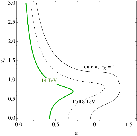
Of course, it is impossible to predict if the central values will remain the same or shift when more data is analyzed. For concreteness, it is interesting to estimate how well the mixing angle can be constrained under the assumption that the rate measurements will converge towards the SM predictions. To illustrate this, in Fig. 5 we show three curves in the $\alpha$ – $x_{u}$ plane. As in Fig. 1, we set $x_{d}=0$ , $y_{u}=y_{d}=1$ , and $c_{G}=c_{W}=c_{B}=0$ . However, instead of using the currently measured signal strengths, we assume that $r_{X,{\rm measured}}=1$ for all channels. The three curves then are the 95% C.L. limits given (i) the current error bars (light solid), (ii) assuming a factor two improvement on the error bars (light dashed), and (iii) expected uncertainties based on the $300~{\rm fb}^{-1}$ 14 TeV ATLAS projections and including an additional factor of two in the statistics assuming that CMS reaches similar sensitivity (green, thick). Note that for the last curve, we only include the channels for which projections are given in [29].

As evident from the plot, the mixing angle $\alpha$ in this scenario could be constrained to $\alpha\,\raisebox{-0.43057pt}{${}_{\textstyle<}\atop{}^{\textstyle\sim}$}\,1.1$ at the end of the 8 TeV run, and to $\alpha\,\raisebox{-0.43057pt}{${}_{\textstyle<}\atop{}^{\textstyle\sim}$}\,0.7$ with data taken at full energy and luminosity. The bounds will thuse become significantly stronger, although they are weakened by the dependence on other parameters such as $x_{\rm u}$ .

With larger available data sets it becomes feasible to constrain CP properties from angular distributions, and the projected sensitivity at the end of the 8 TeV run is similar to Fig. 5 [8]. There are currently no estimates for the angular analysis of decay products of a 125-GeV boson at 14 TeV, but it is likely that it will lead to superior limits compared to Fig. 5, since this method is not affected by the a priori unknown couplings $x_{\rm u,d}$ .

6 Conclusions

The CP properties of the newly discovered boson with mass in the range 125–126 GeV can already be constrained with existing data on production rates and branching ratios. The main reason is that a CP-odd pseudoscalar generally has suppressed couplings to $W$ and $Z$ bosons since such couplings are generated only by higher-dimensional operators. In this paper, the 125-GeV resonance $\phi$ has been assumed to be a general mixture between a CP-even and CP-odd scalar field, and bounds on the mixing angle have been derived in a variety of different scenarios:

(i)

fermion Yukawa couplings fixed to their Standard Model values;
(ii)

the overall scale of up-type and down-type Yukawa couplings to the CP-even and CP-odd components may float freely and independently;
(iii)

the signal peak near 125 GeV is comprised of two particles, $\phi$ and $\phi^{\prime}$ , which are the two mass eigenstates of the mixed CP-even and CP-odd scalar fields;
(iv)

addition of higher-dimensional operators that couple the CP-odd component to gauge bosons;
(v)

a special case of (iv) with vanishing Yukawa couplings (fermiophobic scalar).

Using the most recent Higgs search results released by ATLAS and CMS in July 2012 [1, 2], it turns out that the possibility that $\phi$ is a pure pseudoscalar is already excluded at more than three standard deviations, assuming that the new-physics sector is weakly coupled. Nevertheless, large values of the CP-mixing angles, $\alpha\sim 1.0\dots 1.3$ , are still allowed at the 95% confidence level, although smaller values are in better agreement with the data. Interestingly, a non-zero mixing angle, $\alpha\sim 0.15\dots 0.4$ , together with modified Yukawa couplings, produces a slightly better fit than the Standard Model, although the difference is not significant. If one allows the possibility that two mixed scalars contribute to the observed resonance peak (scenario (iii)), no conclusive constraint on the mixing angle can be derived from current data.

Besides the mixing angle, meaningful limits on the Yukawa couplings and coupling strengths of higher-dimensional operators of $\phi$ have been obtained in all scenarios. The bounds on these parameters and on $\alpha$ are expected to improve significantly with increased statistics, which will lead to more precise measurements of the production rates and branching ratios, as well as open up the possibility to constrain the CP properties by studying angular distributions of the decay products.

Acknowledgements

This project was supported in part by the National Science Foundation under grant PHY-1212635, and by the U.S. Department of Energy, Division of High Energy Physics, under contracts DE-AC02-06CH11357 and DE-FG02-12ER41811.

Appendix

The Lagrangian (4) leads to the following Feynman rules for the coupling of the CP-odd scalar $A$ to SM gauge bosons:

$\displaystyle A\gamma\gamma$	$\displaystyle\frac{c_{\theta}^{2}c_{B}+s_{\theta}^{2}c_{W}}{(4\pi)^{2}v}\epsilon^{\mu\nu\rho\sigma}(p_{2}-p_{3})_{\rho}(p_{1})_{\sigma}\,,$	(29)
$\displaystyle AZZ$	$\displaystyle\frac{s_{\theta}^{2}c_{B}+c_{\theta}^{2}c_{W}}{(4\pi)^{2}v}\epsilon^{\mu\nu\rho\sigma}(p_{2}-p_{3})_{\rho}(p_{1})_{\sigma}\,,$	(30)
$\displaystyle A\gamma Z$	$\displaystyle\frac{s_{\theta}c_{\theta}(c_{W}-c_{B})}{(4\pi)^{2}v}\epsilon^{\mu\nu\rho\sigma}(p_{2}-p_{3})_{\rho}(p_{1})_{\sigma}\,,$	(31)
$\displaystyle AWW$	$\displaystyle\frac{c_{W}}{(4\pi)^{2}v}\epsilon^{\mu\nu\rho\sigma}(p_{2}-p_{3})_{\rho}(p_{1})_{\sigma}\,,$	(32)
$\displaystyle AGG$	$\displaystyle\frac{c_{G}}{(4\pi)^{2}v}\epsilon^{\mu\nu\rho\sigma}(p_{2}-p_{3})_{\rho}(p_{1})_{\sigma}\,,$	(33)

where and $p_{1,2,3}$ are the momenta of the first, second and third particle flowing into the vertex.

References

[1] G. Aad et al. [ATLAS Collaboration], Phys. Lett. B 716, 1 (2012).
[2] S. Chatrchyan et al. [CMS Collaboration], Phys. Lett. B 716, 30 (2012).
[3] G. Davies et al. [Tevatron New Physics Higgs Working Group and CDF and DØ Collaborations], arXiv:1207.0449 [hep-ex].
[4] T. Aaltonen et al. [CDF and DØ Collaborations], Phys. Rev. Lett. 109, 071804 (2012).
[5] J. Ellis and D. S. Hwang, JHEP 1209, 071 (2012);
J. Ellis, R. Fok, D. S. Hwang, V. Sanz and T. You, arXiv:1210.5229 [hep-ph].
[6] S. Y. Choi, M. M. Mühlleitner and P. M. Zerwas, arXiv:1209.5268 [hep-ph].
[7] S. Y. Choi, D. J. Miller, M. M. Mühlleitner and P. M. Zerwas, Phys. Lett. B 553, 61 (2003);
C. P. Buszello, I. Fleck, P. Marquard and J. J. van der Bij, Eur. Phys. J. C 32, 209 (2004);
Y. Gao, A. V. Gritsan, Z. Guo, K. Melnikov, M. Schulze and N. V. Tran, Phys. Rev. D 81, 075022 (2010);
A. De Rujula, J. Lykken, M. Pierini, C. Rogan and M. Spiropulu, Phys. Rev. D 82, 013003 (2010);
R. Boughezal, T. J. LeCompte and F. Petriello, arXiv:1208.4311 [hep-ph].
[8] S. Bolognesi, Y. Gao, A. V. Gritsan, K. Melnikov, M. Schulze, N. V. Tran and A. Whitbeck, arXiv:1208.4018 [hep-ph].
[9] U. De Sanctis, M. Fabbrichesi and A. Tonero, Phys. Rev. D 84, 015013 (2011);
A. Alves, arXiv:1209.1037 [hep-ph].
[10] B. C. Allanach, J. P. Skittrall and K. Sridhar, JHEP 0711, 089 (2007);
J. P. Skittrall, Eur. Phys. J. C 60, 291 (2009);
A. Freitas and P. Schwaller, JHEP 1101, 022 (2011).
[11] K. Hagiwara, Q. Li and K. Mawatari, JHEP 0907, 101 (2009);
H. Murayama and V. Rentala, Phys. Rev. D 85, 095005 (2012).
[12] T. Plehn, D. L. Rainwater and D. Zeppenfeld, Phys. Rev. Lett. 88, 051801 (2002);
V. Hankele, G. Klamke, D. Zeppenfeld and T. Figy, Phys. Rev. D 74, 095001 (2006);
G. Klamke and D. Zeppenfeld, JHEP 0704, 052 (2007);
F. Campanario, M. Kubocz and D. Zeppenfeld, Phys. Rev. D 84, 095025 (2011);
C. Englert, M. Spannowsky and M. Takeuchi, JHEP 1206, 108 (2012).
[13] S. Berge, W. Bernreuther and J. Ziethe, Phys. Rev. Lett. 100, 171605 (2008);
S. Berge and W. Bernreuther, Phys. Lett. B 671, 470 (2009);
S. Berge, W. Bernreuther, B. Niepelt and H. Spiesberger, Phys. Rev. D 84, 116003 (2011).
[14] W. Bernreuther, P. Gonzalez and M. Wiebusch, Eur. Phys. J. C 69, 31 (2010);
G. Burdman, C. E. F. Haluch and R. D. Matheus, Phys. Rev. D 85, 095016 (2012);
B. Holdom, Phys. Lett. B 709, 381 (2012);
M. T. Frandsen and F. Sannino, arXiv:1203.3988 [hep-ph];
J. W. Moffat, arXiv:1204.4702 [hep-ph];
R. S. Chivukula, B. Coleppa, P. Ittisamai, H. E. Logan, A. Martin, J. Ren and E. H. Simmons, arXiv:1207.0450 [hep-ph].
[15] B. Coleppa, K. Kumar and H. E. Logan, Phys. Rev. D 86, 075022 (2012).
[16] V. Barger, P. Langacker, M. McCaskey, M. Ramsey-Musolf and G. Shaughnessy, Phys. Rev. D 79, 015018 (2009).
[17] For a recent review, see G. C. Branco, P. M. Ferreira, L. Lavoura, M. N. Rebelo, M. Sher and J. P. Silva, Phys. Rept. 516, 1 (2012);
and also J. F. Gunion, H. E. Haber, G. L. Kane and S. Dawson, “The Higgs Hunter’s Guide,” Front. Phys. 80, 1 (2000).
[18] A. Barroso, P. M. Ferreira, R. Santos and J. P. Silva, Phys. Rev. D 86, 015022 (2012);
W. Altmannshofer, S. Gori and G. D. Kribs, arXiv:1210.2465 [hep-ph];
S. Chang, S. K. Kang, J.-P. Lee, K. Y. Lee, S. C. Park and J. Song, arXiv:1210.3439 [hep-ph];
Y. Bai, V. Barger, L. L. Everett and G. Shaughnessy, arXiv:1210.4922 [hep-ph].
[19] J. R. Ellis, M. K. Gaillard and D. V. Nanopoulos, Nucl. Phys. B 106, 292 (1976);
M. A. Shifman, A. I. Vainshtein, M. B. Voloshin and V. I. Zakharov, Sov. J. Nucl. Phys. 30, 711 (1979) [Yad. Fiz. 30, 1368 (1979)];
A. Djouadi, M. Spira and P. M. Zerwas, Phys. Lett. B 264, 440 (1991);
M. Spira, A. Djouadi, D. Graudenz and P. M. Zerwas, Nucl. Phys. B 453, 17 (1995).
[20] M. Spira, Fortsch. Phys. 46, 203 (1998).
[21] See $e.\,g.$ sect. 2.1.4 in Ref. [20], and references therein.
[22] A. Belyaev, N. D. Christensen and A. Pukhov, arXiv:1207.6082 [hep-ph].
[23] G. Aad et al. [ATLAS Collaboration], conference note ATLAS-CONF-2012-091.
[24] S. Chatrchyan et al. [CMS Collaboration], conference note CMS-PAS-HIG-12-015.
[25] S. Chatrchyan et al. [CMS Collaboration], conference note CMS-PAS-HIG-12-020.
[26] D. McKeen, M. Pospelov and A. Ritz, arXiv:1208.4597 [hep-ph].
[27] B. Batell, D. McKeen and M. Pospelov, JHEP 1210, 104 (2012).
[28] J. S. Gainer, W.-Y. Keung, I. Low and P. Schwaller, Phys. Rev. D 86, 033010 (2012).
[29] G. Aad et al. [ATLAS Collaboration], conference note ATL-PHYS-PUB-2012-004.