Subfactor projections

The work of Howard Masur and Yair Minsky [12, 13] has served as an inspiration in the study of $Out({\mathbb{F}}_{n})$, the outer automorphism group of the free group ${\mathbb{F}}_{n}$ of rank $n$. Their work starts by proving that the curve complex associated to a compact surface is hyperbolic. There are several established analogs of the curve complex in the $Out({\mathbb{F}}_{n})$ setting that have recently been shown to be hyperbolic, see [3, 7, 11] and [8, Section 8].

The complex ${\mathcal{F}}$ of free factors is the simplicial complex whose vertices are conjugacy classes of nontrivial free factors of ${\mathbb{F}}_{n}$ and a simplex is formed by those vertices that have representatives that can be arranged in a chain. (A subgroup $A$ of ${\mathbb{F}}_{n}$ is a nontrivial free factor if ${\mathbb{F}}_{n}=A*B$ for another subgroup $B$ with $A\neq 1\neq B$.)

The complex ${\mathcal{S}}$ of free splittings, or the sphere complex, or the simplicial completion of Outer space, is the simplicial complex whose $k$-simplices are $(k+1)$-edge free splittings (nontrivial minimal reduced simplicial ${\mathbb{F}}_{n}$-trees with trivial edge stabilizers and $(k+1)$ orbits of edges), up to equivariant isomorphism.

Kapovich-Rafi [9] show how to derive Theorem 1.1 from Theorem 1.2 in a simple way, and Hilion-Horbez [8] give a simpler proof of Theorem 1.2 using surgery paths.

Masur and Minsky also define subsurface projections. If $\alpha$ is a simple closed curve in a surface $S$ and $A$ is a subsurface such that $\alpha$ and $A$ cannot be made disjoint by an isotopy (we also say they intersect), there is a curve $\alpha|A$ in the curve complex of $A$, well defined up to a bounded set, obtained by “closing up the intersection of $\alpha$ and $A$ along the boundary of $A$”. If $A,B$ are two subsurfaces that intersect, one defines the projection $\pi_{A}(B)$ of $B$ to $A$ by taking $\partial B|A$. We view $\pi_{A}(B)$ as a bounded subset of the curve complex of $A$. Masur and Minsky use subsurface projections to estimate distances in mapping class groups, and more generally, to understand their large-scale geometry. To encapsulate this, we first recall a theorem.

In the setting of subsurface projections, $\mathcal{Y}$ will be the collection of curve complexes associated to a collection of pairwise intersecting subsurfaces. That both bullets hold in the setting of subsurface projections (whenever they are both defined) is the work of Masur-Minsky [12, 13] and Behrstock [1]. There is a simple proof of the first bullet due to Leininger, see [10], and of the second bullet in [2].

It is further shown in [2] that there is a finite equivariant coloring of the collection of all subsurfaces of $S$, and the boundaries of two distinct subsurfaces with the same color intersect. Applying Theorem 1.3 to each color separately and then taking the cartesian product one obtains:

The second statement in the theorem recasts the Masur-Minsky distance estimate.

The goal of this paper is to take a step in this direction in the $Out({\mathbb{F}}_{n})$ setting. If $A$ and $B$ are distinct conjugacy classes of nontrivial free factors, we attempt to define $\pi_{A}(B)$, a bounded subset of the splitting complex ${\mathcal{S}}(A)$ of $A$. We start with a simplicial ${\mathbb{F}}_{n}$-tree $T$ representing a splitting of ${\mathbb{F}}_{n}$ where $B$ fixes a vertex. Restricting the action to $A$ and passing to the minimal subtree (assuming $A$ does not fix a vertex of $T$) gives a splitting of $A$. Different choices of $T$ will in general produce unbounded sets in ${\mathcal{S}}(A)$, but when $A$ and $B$ are in “general position” the ambiguity is bounded.

The Main Theorem is proved in Section 4. We thus obtain an isometric action of $Out({\mathbb{F}}_{n})$ on a finite product of hyperbolic spaces. However, orbit maps are not quasi-isometric embedding. We discuss this further in Section 6.

The key to understanding the projections is the analysis of a path in Outer space ${\mathcal{X}}(A)$ of $A$ induced by a path $G_{t}$ in ${\mathcal{X}}$. Here is a motivating example. For a review of the terminology, see Section 2.

Consider the automorphism $\Phi$ of ${\mathbb{F}}_{3}=\langle x,y,z\rangle$ given by $\phi:{\mathbb{F}}_{3}\to{\mathbb{F}}_{3}$, $x\mapsto y$, $y\mapsto z$ and $z\mapsto zx$. The map on the rose $R_{0}$ with loops representing $x,y,z$ is a train track map for $\Phi$. The vertex has 4 gates, namely $\{x,y,z\},\{X\},\{Y\}$ and $\{Z\}$ (the direction oriented the same way as the edge $x$ is also called $x$; the direction pointing the opposite way is $X$ etc). The dilatation $\lambda$ of $\Phi$ satisfies $\lambda^{3}-\lambda^{2}-1=0$ and $\lambda=1.46557\cdots$. The lengths of edges $x,y,z$ are proportional to $1,\lambda,\lambda^{2}$.

Let $A=\langle x,y\rangle$. We are interested in picturing the core of the covering space corresponding to $A$ of the graphs $R_{k}=R_{0}\Phi^{k}$, which we view as a discrete path in ${\mathcal{X}}$ as $k\in{\mathbb{Z}}$ (but one can extend it to an axis $R_{k}$, $k\in{\mathbb{R}}$ of $\Phi$). This core has an induced metric and the structure of legal and illegal turns. Since $\ell_{R_{0}\Phi^{k}}(\gamma)=\ell_{R_{0}}(\Phi^{k}(\gamma))$, this amounts to picturing the $\phi^{k}(A)$-cover of $R_{0}$. See Figure 1.

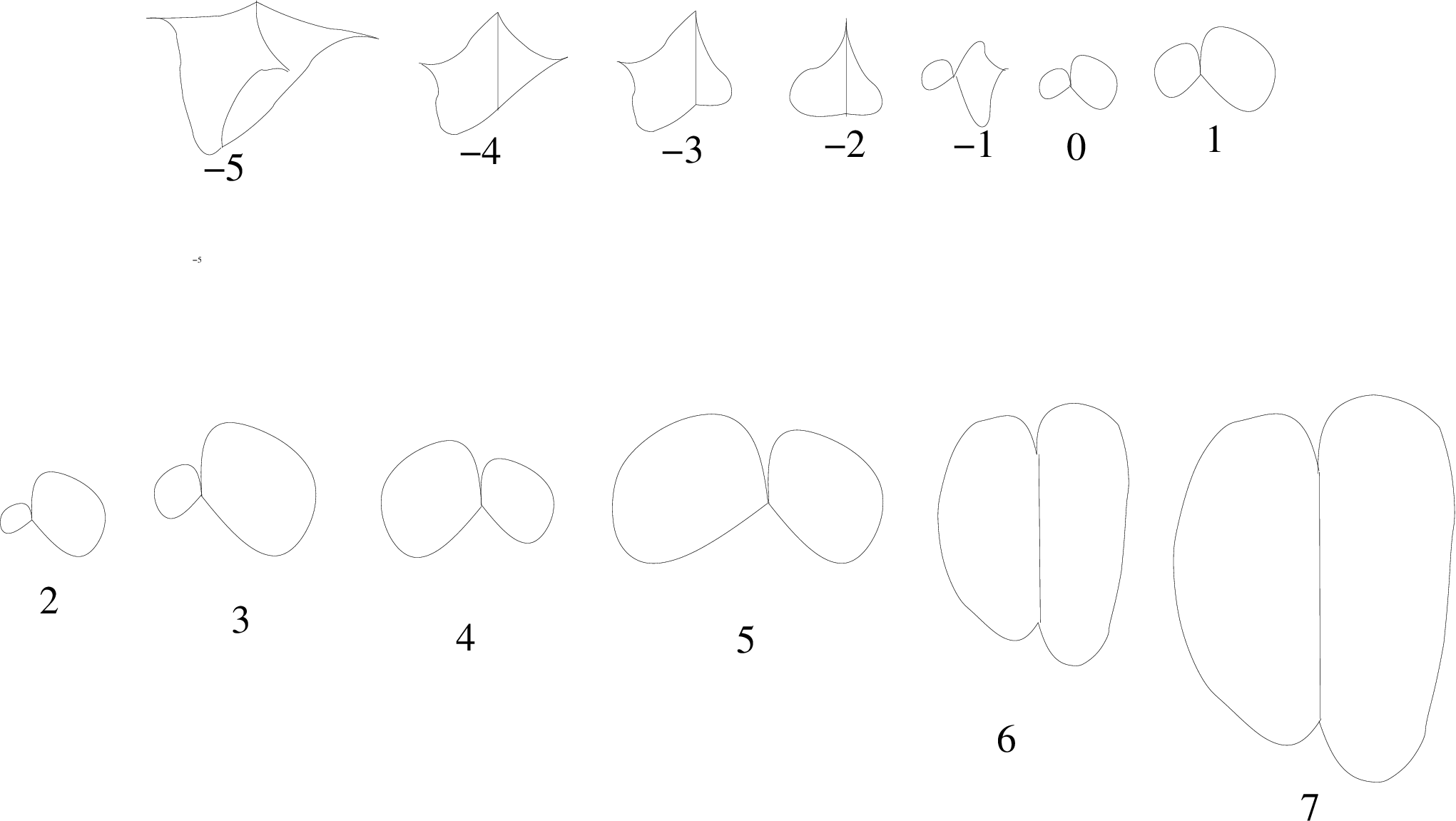
For example, for $k=2$ we compute $\phi^{2}(A)=\langle z,xz\rangle=\langle x,z\rangle$, and for $k=6$ we get $\phi^{6}(A)=\langle zxyzzx,zxyzzxzxy\rangle=\langle zxy,zzx\rangle$ which is represented by a theta graph with the middle edge $z$ going up, the left edge $xy$ and the right edge $zx$, both going down. The illegal turn is at the top.

The reader should note the following features:

• •

  As $k\to\infty$ the volume of $A|R_{k}$ goes to $\infty$ and in fact the topological edges of $A|R_{k}$ are legal and grow exponentially.

• •

  As $k\to-\infty$ the volume of $A|R_{k}$ goes to $\infty$. The topological edges consist of an exponentially growing number of legal segments of length $<2$ and the turns between consecutive such segments are illegal.

Our two main technical lemmas restrict the interval where $A|R_{k}$ can make progress in ${\mathcal{S}}(A)$. Lemma 3.1 says:

• •

  If $A|R_{k}$ has an illegal turn in a topological edge or a vertex with one gate, then the image of $A|R_{t}$, $t\in(-\infty,k]$, in ${\mathcal{S}}(A)$ is uniformly bounded.

• •

  If $A|R_{k}$ has a legal segment of length 2 in a topological edge, then the image of $A|R_{t}$, $t\in[k,\infty)$, in ${\mathcal{S}}(A)$ is uniformly bounded.

An easy computation shows that the first bullet holds for $k=-1$ and the second for $k=9$. Thus all the progress in ${\mathcal{S}}(A)$ is restricted to the interval $[-1,9]$. Lemma 4.4 shrinks this interval further: if every edge of $R_{k}$ has at least two lifts to $A|R_{k}$ then the image of $A|R_{t}$, $t\in[k,\infty)$, in ${\mathcal{S}}(A)$ is uniformly bounded. In our example this holds for $k=7$.

To simplify the analysis, we will work with greedy folding paths as we did in [3]. The above path (an axis of $\Phi$) is not a greedy folding path since not all illegal turns are folding. For example, we will argue in the proof of Lemma 3.1 that if $A|G_{t_{0}}$ has an interior illegal turn then the same is true for all $A|G_{t}$ for $t<t_{0}$. Note that this fails for our path $R_{k}$.

We conclude the paper with the Bounded geodesic image theorem, analogous to the theorem of Masur and Minsky [13].

Sabalka and Savchuk in [14] define a different notion of projection in the language of sphere systems. It is a partially defined map from the sphere complex of $M=\#_{1}^{n}S^{1}\times S^{2}$ to the sphere complex of a submanifold of $M$ which is a complementary component of a sphere system. They also prove versions of the Behrstock inequality and the Bounded geodesic image theorem. It would be interesting to understand the precise relationship between the two notions of projection.

A technical tool we use is that folding paths in Outer space project to reparametrized quasi-geodesics in the splitting complex ${\mathcal{S}}$. In [7] Handel and Mosher use a special kind of folding paths (maximal folds on maps with at least 3 gates at every vertex) that does not suffice for our purposes. In the appendix we follow the same outline as in [7] but we use (liberal) folding paths. Interestingly, the proof becomes simpler since we do not have to arrange the 3 gates condition after every modification.

Acknowledgements. We thank Ken Bromberg, Ursula Hamenstädt, Ilya Kapovich and Patrick Reynolds for their interest and useful comments.

In this section we recall basic definitions and facts about Outer space with an emphasis on folding paths. For more information see [3].

A graph is a 1-dimensional CW complex. The rose in rank $n$ is the graph $R_{n}$ with 1 vertex and $n$ edges. A finite connected graph is a core graph if it has no valence 1 vertices. The core of a connected graph $\Gamma$ with finitely generated $\pi_{1}(\Gamma)$ is the unique core graph $C\subset\Gamma$ so that inclusion is a homotopy equivalence.

A marking of a graph $\Gamma$ is a homotopy equivalence $f:R_{n}\to\Gamma$. A metric on a graph $\Gamma$ is a function that assigns a positive number $\ell(e)$, called length, to each edge $e$ of $\Gamma$. A metric allows one to view $\Gamma$ as a path metric space. Culler-Vogtmann’s Outer space ${\mathcal{X}}$ is the space of equivalence classes of triples $(\Gamma,\ell,f)$ where $\Gamma$ is a finite graph with no vertices of valence 1 or 2, $f$ is a marking, and $\ell$ is a metric on $\Gamma$ with volume (i.e. sum of the lengths of all edges) equal to 1. Two such triples $(\Gamma,\ell,f)$ and $(\Gamma^{\prime},\ell^{\prime},f^{\prime})$ are equivalent if there is an isometry $\phi:\Gamma\to\Gamma^{\prime}$ such that $\phi f\simeq f^{\prime}$ (homotopic).

The group $Out({\mathbb{F}}_{n})$ can be identified with the group of homotopy equivalences on $R_{n}$. The action of $Out({\mathbb{F}}_{n})$ on ${\mathcal{X}}$ (on the right) is defined by changing the marking: $[(\Gamma,\ell,f)]\cdot\Phi=[(\Gamma,\ell,f\Phi)]$.

We frequently simplify the notation and replace the equivalence class $[(\Gamma,\ell,f)]$ by $\Gamma$.

The set $\mathcal{C}$ of nontrivial conjugacy classes in ${\mathbb{F}}_{n}$ can be identified with the set of homotopy classes of immersed loops in $R_{n}$. If $\alpha\in\mathcal{C}$ and $[\Gamma,\ell,f)]\in{\mathcal{X}}$, we define $\alpha|\Gamma$ to be the immersed loop homotopic to $f(\alpha)$, and we let $\ell_{\Gamma}(\alpha)$ be the length of $\alpha|\Gamma$. We then have $\ell_{\Gamma\Phi}(\alpha)=\ell_{\Gamma}(\Phi(\alpha))$.

If $\Gamma,\Gamma^{\prime}\in{\mathcal{X}}$ we say that a map $\phi:\Gamma\to\Gamma^{\prime}$ is a difference of markings if $\phi f\simeq f^{\prime}$. We will normally consider only maps that are linear (constant speed) on each edge. Denote by $\sigma(\phi)$ the Lipschitz constant of $\phi$, i.e. the maximum speed over all edges of $\Gamma$. The Lipschitz distance is defined by

where the minimum is taken over all difference of markings maps $\phi:\Gamma\to\Gamma^{\prime}$.

A train track structure on a graph $\Gamma$ consists of an equivalence relation on the set of directions out of each vertex of $\Gamma$. One usually pictures graphs with a train track structure so that equivalent directions are tangent. Equivalence classes are called gates. The tension graph $\Delta_{\phi}$ has a natural train track structure, where two directions $d_{1},d_{2}$ out of a vertex $v\in\Delta_{\phi}$ are equivalent if they are mapped by $\phi$ to the same direction out of $\phi(v)$ (which is not required to be a vertex). We say $\phi$ is optimal if $\Delta_{\phi}=\Gamma$ and there are at least two gates at every vertex of $\Gamma$. A turn (i.e. a pair of distinct directions out of a vertex) is illegal if the directions are in the same gate, and otherwise it is legal. An immersed path or a loop is legal if it takes only legal turns.

An optimal map $\phi:\Gamma\to\Gamma$ is a train track map if there is a train track structure on $\Gamma$ which is preserved by $\phi$, in the sense that legal paths are mapped to legal paths.

Now let $\phi:\Gamma\to\Gamma^{\prime}$ be optimal. We define a (greedy) folding path induced by $\phi$ as follows. It is the unique (up to reparametrization) path $G_{t}$, $t\in[\alpha,\omega]$ with $G_{\alpha}=\Gamma$, $G_{\omega}=\Gamma^{\prime}$, and for every $t\in[\alpha,\omega)$ there is $\epsilon>0$ such that for every $\tau\in[t,t+\epsilon]$ the graph $G_{\tau}$ is obtained from $G_{t}$ by identifying segments of length $\tau-t$ leaving any vertex in equivalent directions and then rescaling to restore volume 1. We normally parametrize the path by arclength, i.e. so that for $t_{1}<t_{2}$ we have $d(G_{t_{1}},G_{t_{2}})=t_{2}-t_{1}$. There are induced optimal maps $G_{t_{1}}\to G_{t_{2}}$ for $t_{1}<t_{2}$ and they compose naturally.

If $\phi:G\to G^{\prime}$ is any difference of markings map there is an induced path from $G$ to $G^{\prime}$ as follows. It is a concatenation of a linear path within a simplex from $G\to G^{\prime\prime}$ and a folding path from $G^{\prime\prime}$ to $G^{\prime}$ induced by an optimal map (see [6], also [3, Proposition 2.7]).

Let $G_{t}$ be a folding path defined on a closed interval $[\alpha,\omega]$. Then the interval can be subdivided into finitely many subintervals $[t_{i},t_{i+1}]$ so that for every $t\in(t_{i},t_{i+1})$ all illegal turns are at vertices with two gates, with one gate consisting of a single direction. Moreover, all $G_{t}$ in this interval are canonically homeomorphic with the homeomorphism preserving the train track structure. As $t$ increases in this open interval, $G_{t}$ moves along a straight line in the interior of a simplex in ${\mathcal{X}}$, i.e. only the lengths of the edges change. See Figure 2.

The proof of these facts follows from the analysis of folding paths in [3]. We understand what happens to the right of a given $G_{t}$, by the definition of a folding path. To understand what happens on an interval $[t_{0}-\epsilon,t_{0}]$ we use the local description of unfolding in [3, Section 4].

Let $N$ be a small connected neighborhood of a vertex $v$ in $G_{t_{0}}$. Thus $N$ is a wedge of arcs along their endpoints, with $v$ the wedge point. For small $\epsilon>0$ the preimage $N_{\epsilon}\subset G_{t_{0}-\epsilon}$ of $N$ is a tree that comes with a height function and a collection of widgets. See Figure 3.

The preimages of $v$ are at height 0. All illegal turns are at the vertices at height $\epsilon$. Each of these vertices has two gates, one gate consists of a single direction drawn upwards and the other gate has $\geq 2$ directions all of which fold together at $t=t_{0}$. The union of the edges in the downwards gate at each vertex at height $\epsilon$ is a widget. The union of all widgets is a tree.

We also recall that there are coarse projection maps ${\mathcal{X}}\to{\mathcal{S}}\to{\mathcal{F}}$ defined by sending a graph $\Gamma\in{\mathcal{X}}$ to a 1-edge splitting of ${\mathbb{F}}_{n}$ obtained by collapsing all but one edge of $\Gamma$, and sending a 1-edge splitting to a vertex stabilizer. A useful fact, supplementing Theorems 1.1 and 1.2, is that the image of a folding path in ${\mathcal{X}}$ is a reparametrized quasi-geodesic in both ${\mathcal{F}}$ and ${\mathcal{S}}$, with uniform constants (see [3] for ${\mathcal{F}}$ and the appendix of this paper for ${\mathcal{S}}$).

Recall that $A|G$ denotes the core of the covering space of $G$ corresponding to a subgroup $A$ of ${\mathbb{F}}_{n}$. In this section we prove two technical lemmas about induced paths. The setting in both is that $G_{t}$ is a folding path in ${\mathcal{X}}$, $A|G_{t}$ is the induced path in Outer space ${\mathcal{X}}(A)$ of $A$, and we are interested in identifying geometrically the portions of the path $A|G_{t}$ where it (possibly) makes progress in the splitting complex ${\mathcal{S}}(A)$ of $A$.

By a topological (or natural) edge in a core graph we mean an edge with respect to the cell structure with all vertices of valence $\geq 3$, and likewise, vertices with valence $\geq 3$ are natural (when the core graph is a circle we don’t talk about topological edges). An interior illegal turn is the turn (pair of directions) at a valence two vertex with one gate. Such turns arise in $A|G_{t}$.

Let $G_{t}$ be a folding path. We say that a collection of subgraphs $H_{t}\subset G_{t}$ is forward invariant if for every $t<t^{\prime}$ the folding map $G_{t}\to G_{t^{\prime}}$ takes $H_{t}$ into $H_{t^{\prime}}$.

We will denote by $\Theta_{t}$ the image of $A|G_{t}\to G_{t}$, by $\Omega_{t}\subset G_{t}$ the set of points with at least two preimages in $A|G_{t}$, and by $\tilde{\Omega}_{t}\subset A|G_{t}$ the preimage of $\Omega_{t}$ in $A|G_{t}$.

From now on we restrict $G_{t}$ to the middle segment of Lemma 3.1.

References

- [1] Jason A. Behrstock. Asymptotic geometry of the mapping class group and Teichmüller space. Geom. Topol., 10:1523–1578, 2006.
- [2] Mladen Bestvina, Kenneth Bromberg, and Koji Fujiwara. Constructing group actions on quasi-trees and applications to mapping class groups. arXiv:1006.1939.
- [3] Mladen Bestvina and Mark Feighn. Hyperbolicity of the complex of free factors. arXiv:1107.3308.
- [4] Mladen Bestvina, Mark Feighn, and Michael Handel. The Tits alternative for . I. Dynamics of exponentially-growing automorphisms. Ann. of Math. (2), 151(2):517–623, 2000.
- [5] Mladen Bestvina and Michael Handel. Train tracks and automorphisms of free groups. Ann. of Math. (2), 135(1):1–51, 1992.
- [6] Stefano Francaviglia and Armando Martino. Metric properties of Outer space. Pub. Mat., 55:433–473, 2011.
- [7] Michael Handel and Lee Mosher. The free splitting complex of a free group I: Hyperbolicity. arXiv:1111.1994.
- [8] Arnaud Hilion and Camille Horbez. The hyperbolicity of the sphere complex via surgery paths. arXiv:1210.6183.
- [9] Ilya Kapovich and Kasra Rafi. On hyperbolicity of free splitting and free factor complexes. arXiv:1206.3626.
- [10] Johanna Mangahas. Uniform uniform exponential growth of subgroups of the mapping class group. Geom. Funct. Anal., 19(5):1468–1480, 2010.
- [11] Brian Mann. Hyperbolicity of the cyclic splitting complex. arXiv:1212.2986.
- [12] Howard A. Masur and Yair N. Minsky. Geometry of the complex of curves. I. Hyperbolicity. Invent. Math., 138(1):103–149, 1999.
- [13] Howard A. Masur and Yair N. Minsky. Geometry of the complex of curves. II. Hierarchical structure. Geom. Funct. Anal., 10(4):902–974, 2000.
- [14] Lucas Sabalka and Dmytro Savchuk. Submanifold projection. arXiv:1211.3111.
- [15] John R. Stallings. Topology of finite graphs. Invent. Math., 71(3):551–565, 1983.