跳到论文正文
W Papers独立论文阅读器 arXiv:1211.1660 论文正文 计算阅读时间 · 0%
引用这篇论文根据当前论文元数据生成,正式投稿前建议核对。


License: arXiv.org perpetual non-exclusive license
arXiv:1211.1660v1 [cs.IT] 07 Nov 2012

Secret-Key Agreement Capacity over Reciprocal Fading Channels: A Separation ApproachThanks: This work was supported by a Discovery Grant from the Natural Sciences Engineering Research Council (NSERC) of Canada.

Ashish Khisti Affiliation:  Affiliation: Dept. of Electrical and Computer Engineering
University of Toronto
Toronto, ON, Canada
Email: akhisti@comm.utoronto.ca
Affiliation: 
Abstract

Fundamental limits of secret-key agreement over reciprocal wireless channels are investigated. We consider a two-way block-fading channel where the channel gains in the forward and reverse links between the legitimate terminals are correlated. The channel gains between the legitimate terminals are not revealed to any terminal, whereas the channel gains of the eavesdropper are revealed to the eavesdropper. We propose a two-phase transmission scheme, that reserves a certain portion of each coherence block for channel estimation, and the remainder of the coherence block for correlated source generation. The resulting secret-key involves contributions of both channel sequences and source sequences, with the contribution of the latter becoming dominant as the coherence period increases. We also establish an upper bound on the secret-key capacity, which has a form structurally similar to the lower bound. Our upper and lower bounds coincide in the limit of high signal-to-noise-ratio (SNR) and large coherence period, thus establishing the secret-key agreement capacity in this asymptotic regime. Numerical results indicate that the proposed scheme achieves significant gains over training-only schemes, even for moderate SNR and small coherence periods, thus implying the necessity of randomness-sharing in practical secret-key generation systems.

I Introduction

Physical layer can provide a valuable resource for enhancing security and confidentiality of wireless communication systems. One promising method that has received a significant interest in recent years (see e.g., [1, 2, 3, 4, 5, 6, 7, 8, 9, 10, 11, 12, 13, 14, 15, 16, 17, 18, 19, 20] and the references therein) is the generation of a shared secret key using channel reciprocity. When the terminals use identical carrier frequencies, a physical reciprocity [21] exists between uplink and downlink channels, which provides a natural mechanism for key exchange. The terminals first transmit training signals to estimate the underlying channel gains, then agree on a common sequence using error correction, and finally distill a shared secret-key from this common sequence. A number of experimental testbeds already demonstrate practical viability of such methods. See e..g., [13, 18, 19, 20].

Despite this growing interest, information theoretic limits of secret-key agreement over wireless channels have not received much attention. Consider a block-fading channel where the channel gains are sampled once every coherence period and remain constant during the coherence block. Clearly, channel reciprocity alone achieves a rate that vanishes as the coherence period increases. What form of signalling within each coherence block maximizes the secret-key rate? To our knowledge, only a recent paper [22] considers this question. The authors consider a separation based scheme. A portion of each coherence block is reserved for transmission of pilot symbols to estimate the channel coefficients. The remainder of the coherence block is used for transmission of a confidential-message. Unfortunately the authors observe that one cannot separately tune the two phases. Any rate/power adaptation done during the message transmission phase, leaks information about the channel gains to an eavesdropper and in turn reduce the contribution from reciprocity. As such the wiretap code for confidential message transmission proposed in [22] does not involve any rate or power adaptation. It achieves a non-zero rate only if we impose that the eavesdropper’s channel on average be weaker than the legitimate receiver’s channel. If this condition is not satisfied, the secret-key rate achieved in [22] reduces to the rate achieved using a training only scheme and vanishes to zero as the coherence period becomes large.

In the present paper we too consider a separation based scheme, but substitute the confidential-message transmission phase with a different communication strategy — randomness sharing. Following the training phase, in each coherence block the terminals exchange i.i.d. random variables to generate correlated source sequences between the terminals. No power allocation is performed during this phase, yet it results in a positive secret-key rate even when the eavesdropper’s channel is on average stronger than the legitimate receiver’s channel. We note that the randomness sharing scheme for secret-key generation has been investigated in several previous works (see e.g., [23, 24, 25, 26, 27, 28] and references therein). However to the author’s knowledge, the present paper appears to be the first attempt that studies randomness sharing, in conjunction with training techniques, in non-coherent wireless channels. Furthermore our proposed scheme has several appealing features. First it achieves a rate that does not vanish in the large coherence-period limit, thus making it attractive in this practically relevant regime. Secondly our proposed separation scheme is asymptotically optimal among all signalling schemes in the two-way fading channel. In particular, we also establish an upper bound on the secret-key agreement capacity in the proposed setup. The upper bound expression is structurally similar to the lower bound expression and furthermore the difference between our upper and lower bound vanishes to zero in the limit of large coherence period and high signal-to-noise-ratio, thus establishing an asymptotic capacity result. Numerical results indicate that even for moderate SNR and relatively small coherence periods the gains resulting from randomness sharing are significant over training-only schemes.

Our proposed model also differs from reference [22] in that we only assume imperfect reciprocity in uplink and downlink channels i.e., we assume that the channel gains in uplink and downlink are correlated, but not identical. In general achieving perfect channel reciprocity in baseband is challenging because different terminals use different I/Q mixers, amplifiers and path lengths in the RF chains. While closed-loop calibration can be performed (see e.g. [29, 30]), such methods can become challenging if the calibration needs to be done in the open air. Hence we believe that our assumption of imperfect reciprocity may perhaps be more realistic in practice. Nevertheless we also note that our coding technique can also be applied to the case of perfect reciprocity, and improves upon the message transmission scheme [22].

In other related works, an information theoretic framework for secure communication was pioneered by Shannon [31]. The problem of secret-key generation from common randomness between two legitimate terminals was introduced in [23, 24]. The setup considered in these papers involves one-way communication channel models and a public-discussion channel. In followup works, secret-key agreement capacity over one-way fading channels with a noiseless public feedback link have been studied in e.g. [32, 33, 34, 35, 36]. References [37, 38, 39] study secret-key agreement over a channel with two-sided state sequence, which has application to fading channels. However these works do not incorporate the cost of acquiring channel state information which is of critical importance in the proposed setup.

II System Model and Main Results

Fig. 1: Problem Setup. There are two legitimate terminals and one eavesdropper terminal. The legitimate terminals AA and BB are required to agree on a common secret-key. The fading gains 𝘩A​B{\mathssf{h}}_{AB} and 𝘩B​A{\mathssf{h}}_{BA} are not revealed to any terminals, whereas the 𝘨A​E{\mathssf{g}}_{AE} and 𝘨B​E{\mathssf{g}}_{BE} are revealed to the eavesdropper.

As illustrated in Fig. 1, we consider a setup with two legitimate terminals AA and BB and one eavesdropper EE. The terminals AA and BB communicate over a two-way non-coherent wireless channel:

𝘺B​(t)=𝘩A​B​(t)​𝘹A​(t)+𝘯B​(t),𝘺A​(t)=𝘩B​A​(t)​𝘹B​(t)+𝘯A​(t),\displaystyle{\mathssf{y}}_{B}(t)\!=\!{\mathssf{h}}_{AB}(t){\mathssf{x}}_{A}(t)\!+\!{\mathssf{n}}_{B}(t),~{\mathssf{y}}_{A}(t)\!=\!{\mathssf{h}}_{BA}(t){\mathssf{x}}_{B}(t)\!+\!{\mathssf{n}}_{A}(t), (1)
𝘻A​E​(t)=𝘨A​E​(t)​𝘹A​(t)+𝘯A​E​(t),𝘻B​E​(t)=𝘨B​E​(t)​𝘹B​(t)+𝘯B​E​(t)\displaystyle{\mathssf{z}}_{AE}(t)\!\!=\!\!{\mathssf{g}}_{AE}(t){\mathssf{x}}_{A}(t)\!+\!{\mathssf{n}}_{AE}(t),~{\mathssf{z}}_{BE}(t)\!\!=\!\!{\mathssf{g}}_{BE}(t){\mathssf{x}}_{B}(t)\!+\!{\mathssf{n}}_{BE}(t) (2)

where t∈{1,…,N}t\in\{1,\ldots,N\} denotes the time index, 𝘺A​(t){\mathssf{y}}_{A}(t) and 𝘺B​(t){\mathssf{y}}_{B}(t) denote the output symbols at terminals AA and BB and {𝘻A​E​(t),𝘻B​E​(t)}\{{\mathssf{z}}_{AE}(t),{\mathssf{z}}_{BE}(t)\} denote the output symbols at terminal EE. The input symbols generated by terminals AA and BB at time tt are denoted by 𝘹A​(t){\mathssf{x}}_{A}(t) and 𝘹B​(t){\mathssf{x}}_{B}(t) respectively and are required to satisfy the average power constraints:

1N​∑t=1NE⁡[|𝘹A​(t)|2]≤P,1N​∑t=1NE⁡[|𝘹B​(t)|2]≤P\displaystyle\frac{1}{N}\sum_{t=1}^{N}E[|{\mathssf{x}}_{A}(t)|^{2}]\leq P,\quad\frac{1}{N}\sum_{t=1}^{N}E[|{\mathssf{x}}_{B}(t)|^{2}]\leq P

The channel gains (𝘩A​B,𝘩B​A,𝘨A​E,𝘨B​E)({\mathssf{h}}_{AB},{\mathssf{h}}_{BA},{\mathssf{g}}_{AE},{\mathssf{g}}_{BE}) are drawn from a distribution p⁡(𝘩A​B,𝘩B​A)​p​(𝘨A​E,𝘨B​E)p({{\mathssf{h}}_{AB},{\mathssf{h}}_{BA}})p({\mathssf{g}}_{AE},{\mathssf{g}}_{BE}) once every TT consecutive symbols and stay constant over this period i.e., the channel gains remain constant in the interval t∈[i​T+1,(i+1)​T]t\in[iT+1,(i+1)T] for i=0,1,…,NT−1i=0,1,\ldots,\frac{N}{T}-1. We assume that the channel gains 𝘩A​B​(t){\mathssf{h}}_{AB}(t) and 𝘩B​A​(t){\mathssf{h}}_{BA}(t) are not revealed to any of the terminals apriori, whereas the channel gains (𝘨A​E​(t),𝘨B​E​(t))({\mathssf{g}}_{AE}(t),{\mathssf{g}}_{BE}(t)) are revealed to the eavesdropper terminal. The additive noise variables are drawn from an i.i.d. 𝒞​𝒩​(0,1){\mathcal{CN}}(0,1) distribution. When computing the achievable rates, for convenience, we will assume that the channel gains are all drawn from the Gaussian 𝒞​𝒩​(0,1){\mathcal{CN}}(0,1) distribution, although our results are not tied to this assumption.

Remark 1

While we assume that the channel gains of the eavesdropper are independent of (𝘩A​B,𝘩B​A)({\mathssf{h}}_{AB},{\mathssf{h}}_{BA}), our results naturally extend to the case when the channel gains are drawn from a joint distribution p⁡(𝘩A​B,𝘩B​A,𝘨A​E,𝘨B​E)p({\mathssf{h}}_{AB},{\mathssf{h}}_{BA},{\mathssf{g}}_{AE},{\mathssf{g}}_{BE}). Also note that the eavesdropper observes the transmission from the two terminals AA and BB over non-interfering links. An eavesdropper who observes a superposition of the two signals can only be weaker than the proposed eavesdropper.

Definition 1 (Secret-Key Capacity)

A feasible secret-key generation protocol is defined as follows. Terminals AA and BB sample independent random variables 𝘮A{\mathssf{m}}_{A} and 𝘮B{\mathssf{m}}_{B} from a product distribution p⁡(𝘮A)​p​(𝘮B)p({\mathssf{m}}_{A})p({\mathssf{m}}_{B}). At time t,t, terminals AA and BB generate the symbols 𝘹A​(t)=fA​(𝘮A,𝘺At−1){\mathssf{x}}_{A}(t)=f_{A}({\mathssf{m}}_{A},{\mathssf{y}}_{A}^{t-1}) and 𝘹B​(t)=fB​(𝘮B,𝘺Bt−1){\mathssf{x}}_{B}(t)=f_{B}({\mathssf{m}}_{B},{\mathssf{y}}_{B}^{t-1}). At the end of NN channel uses, the terminals AA and BB generate secret keys 𝘬A{\mathssf{k}}_{A} and 𝘬B{\mathssf{k}}_{B} respectively using the functions 𝘬A=𝒦A​(𝘺AN,𝘮A){\mathssf{k}}_{A}={\mathcal{K}}_{A}({\mathssf{y}}_{A}^{N},{\mathssf{m}}_{A}) and 𝘬B=𝒦B​(𝘺BN,𝘮B){\mathssf{k}}_{B}={\mathcal{K}}_{B}({\mathssf{y}}_{B}^{N},{\mathssf{m}}_{B}). We require that Pr⁡(𝘬A≠𝘬B)≤εN\Pr({\mathssf{k}}_{A}\neq{\mathssf{k}}_{B})\leq\varepsilon_{N} and furthermore 1N​I​(𝘬A,𝘇N,𝗴K)≤εN\frac{1}{N}I({\mathssf{k}}_{A};{\mathbsf{z}}^{N},{\mathbsf{g}}^{K})\leq\varepsilon_{N} for some sequence εN\varepsilon_{N} that goes to zero as N→∞N\rightarrow\infty. The largest achievable rate R=1N​H​(𝘬A)R=\frac{1}{N}H({\mathssf{k}}_{A}) is denoted as the secret-key capacity. □\hfill\Box

As our main result, we establish upper and lower bounds on the secret-key capacity for the two-way non-coherent channel model.

II-A Upper Bound

Theorem 1

An upper-bound on the secret-key capacity of the two-way non-coherent fading channel is,

C≤R+=1T​I​(𝘩A​B,𝘩B​A)+max{P⁡(𝘩A​B)}∈𝒫A​B{I(𝘺B;𝘹A|𝘩A​B,𝘻A​E,𝘨A​E)}+max{P⁡(𝘩B​A)}∈𝒫B​A{I(𝘺A;𝘹B|𝘩B​A,𝘻B​E,𝘨B​E)},C\leq R^{+}=\frac{1}{T}I({\mathssf{h}}_{AB};{\mathssf{h}}_{BA})+\\ \max_{\{P({\mathssf{h}}_{AB})\}\in{\mathcal{P}}_{AB}}\left\{I({\mathssf{y}}_{B};{\mathssf{x}}_{A}|{\mathssf{h}}_{AB},{\mathssf{z}}_{AE},{\mathssf{g}}_{AE})\right\}\\ +\max_{\{P({\mathssf{h}}_{BA})\}\in{\mathcal{P}}_{BA}}\left\{{I({\mathssf{y}}_{A};{\mathssf{x}}_{B}|{\mathssf{h}}_{BA},{\mathssf{z}}_{BE},{\mathssf{g}}_{BE})}\right\}, (3)

where the above expression is evaluated for

𝘹A∼𝒞​𝒩​(0,P⁡(𝘩A​B)),𝘹B∼𝒞​𝒩​(0,P⁡(𝘩B​A)),\displaystyle{\mathssf{x}}_{A}\sim{\mathcal{CN}}(0,P({{\mathssf{h}}_{AB}})),~{\mathssf{x}}_{B}\sim{\mathcal{CN}}(0,P({\mathssf{h}}_{BA})),

and the set 𝒫A​B{\mathcal{P}}_{AB} is the set of all non-negative power allocation functions P⁡(𝘩A​B)P({{\mathssf{h}}_{AB}}) that satisfy the average power constraint E⁡[P⁡(𝘩A​B)]≤PE[P({\mathssf{h}}_{AB})]\leq P and the set 𝒫B​A{\mathcal{P}}_{BA} is defined similarly.

Remark 2

The upper bound expression in Theorem 1 has a natural interpretation. The term 1T​I​(𝘩A​B,𝘩B​A)\frac{1}{T}I({\mathssf{h}}_{AB};{\mathssf{h}}_{BA}) is the contribution arising from reciprocal channel gains. The second term is the secret key rate achieved over a one way fading channel

𝘺B=𝘩A​B​𝘹A+𝘯B,𝘻A​E=𝘨A​E​𝘹A+𝘯A​E\displaystyle{\mathssf{y}}_{B}={\mathssf{h}}_{AB}{\mathssf{x}}_{A}+{\mathssf{n}}_{B},\quad{\mathssf{z}}_{AE}={\mathssf{g}}_{AE}{\mathssf{x}}_{A}+{\mathssf{n}}_{AE} (4)

and a public discussion channel in the reverse link, when the fading chain 𝘩A​B{\mathssf{h}}_{AB} is revealed to all the terminals and the channel gain 𝘨A​E{\mathssf{g}}_{AE} is revealed to the eavesdropper. Likewise the third term is the contribution arising from the one-way fading channel in the reverse link. The upper bound expression (3) indicates that the contribution of these three terms is additive. □\hfill\Box

The proof of Theorem 1 is provided in section III.

II-B Lower Bound - Public Discussion

Fig. 2: Separation-based approach for secret-key generation. In each coherence block of length TT symbols, the first symbol is dedicated to training and a power P1P_{1} is used i.e., 𝘹A​(i​T+1)=𝘹B​(i​T+1)=P1{\mathssf{x}}_{A}(iT+1)={\mathssf{x}}_{B}(iT+1)=\sqrt{P_{1}}. The remaining T−1{T-1} symbols are used for randomness generation. Each symbol is sampled i.i.d. 𝒞​𝒩​(0,P2){\mathcal{CN}}(0,P_{2}) in this phase.

Our proposed coding scheme involves a separation based approach. As shown in Fig. 2, the first symbol in each coherence block is reserved for sending a training symbol and a total power of P1P_{1} is used in this phase. This allows the terminals BB and AA to generate linear minimum mean squared error estimates of the channel gains 𝘩A​B{\mathssf{h}}_{AB} and 𝘩B​A{\mathssf{h}}_{BA} respectively i.e.,

𝘩^A​B=α​𝘩A​B+𝘦A​B\displaystyle\hat{{\mathssf{h}}}_{AB}=\alpha{\mathssf{h}}_{AB}+{\mathssf{e}}_{AB} (5)
𝘩^B​A=α​𝘩B​A+𝘦B​A,\displaystyle\hat{{\mathssf{h}}}_{BA}=\alpha{\mathssf{h}}_{BA}+{\mathssf{e}}_{BA}, (6)

where α=P1P1+1\alpha=\frac{P_{1}}{P_{1}+1} is the estimation coefficient, and 𝘦A​B{\mathssf{e}}_{AB} and 𝘦B​A{\mathssf{e}}_{BA} both have the distribution 𝒞​𝒩​(0,α⁡(1−α)){\mathcal{CN}}\left(0,\alpha(1-\alpha)\right) and are independent of the channel gains 𝘩A​B{\mathssf{h}}_{AB} and 𝘩B​A{\mathssf{h}}_{BA} respectively.

For the reminder of coherence block, both the terminals transmit i.i.d. symbols from 𝒞​𝒩​(0,P2){\mathcal{CN}}(0,P_{2}) to generate correlated source sequences i.e., in coherence period ii each component of the vector 𝘅¯A​(i)∈ℂT−1\bar{{\mathbsf{x}}}_{A}(i)\in{\mathbb{C}}^{T-1} is generated i.i.d. 𝒞​𝒩​(0,P2){\mathcal{CN}}(0,P_{2}) and similarly each component of the vector 𝘅¯B​(i)\bar{{\mathbsf{x}}}_{B}(i) is i.i.d. 𝒞​𝒩​(0,P2){\mathcal{CN}}(0,P_{2}). The corresponding received vectors are given by

𝘆¯A​(i)=𝘩B​A​(i)​𝘅¯B​(i)+𝗻¯B​A​(i),𝘆¯B​(i)=𝘩A​B​(i)​𝘅¯A​(i)+𝗻¯A​B​(i).\displaystyle\bar{{\mathbsf{y}}}_{A}(i)\!\!=\!\!{\mathssf{h}}_{BA}(i)\bar{{\mathbsf{x}}}_{B}(i)\!+\!\bar{{\mathbsf{n}}}_{BA}(i),\bar{{\mathbsf{y}}}_{B}(i)\!\!=\!\!{\mathssf{h}}_{AB}(i)\bar{{\mathbsf{x}}}_{A}(i)\!+\!\bar{{\mathbsf{n}}}_{AB}(i). (7)

At the end of KK such coherence blocks, as indicated in Table I, terminal AA has access to (𝘩^B​AK,𝘅¯AK,𝘆¯AK)(\hat{{\mathssf{h}}}_{BA}^{K},\bar{{\mathbsf{x}}}_{A}^{K},\bar{{\mathbsf{y}}}_{A}^{K}) whereas terminal BB has access to (𝘩^A​BK,𝘅¯BK,𝘆¯BK)(\hat{{\mathssf{h}}}_{AB}^{K},\bar{{\mathbsf{x}}}_{B}^{K},\bar{{\mathbsf{y}}}_{B}^{K}). The eavesdropper observes (𝘨A​EK,𝘨B​EK,𝘇¯A​EK,𝘇¯B​EK)({\mathssf{g}}_{AE}^{K},{\mathssf{g}}_{BE}^{K},\bar{{\mathbsf{z}}}_{AE}^{K},\bar{{\mathbsf{z}}}_{BE}^{K}).

TABLE I: Correlated Source and Channel Sequences at the Terminals
Sequence/Terminal A B E
Channel Sequence 𝘩^B​AK\hat{{\mathssf{h}}}_{BA}^{K} 𝘩^A​BK\hat{{\mathssf{h}}}_{AB}^{K} (𝘨A​EK,𝘨B​EK)({\mathssf{g}}_{AE}^{K},{\mathssf{g}}_{BE}^{K})
Source Sequence - I 𝘅¯AK\bar{{\mathbsf{x}}}_{A}^{K} 𝘆¯BK\bar{{\mathbsf{y}}}_{B}^{K} 𝘇¯A​EK\bar{{\mathbsf{z}}}_{AE}^{K}
Source Sequence - II 𝘆¯AK\bar{{\mathbsf{y}}}_{A}^{K} 𝘅¯BK\bar{{\mathbsf{x}}}_{B}^{K} 𝘇¯B​EK\bar{{\mathbsf{z}}}_{BE}^{K}

These correlated sequences are in turn used to generate a common secret-key by exchanging suitable public messages in the reconciliation phase [23, 24]. As indicated, in this section we assume that these public-messages for secret-key generation are transmitted over an external public discussion channel. The resulting rate-expression is simpler and has a form that can be immediately compared with the upper bound. Subsequently we will remove this assumption and consider the transmission of public messages directly over the wireless channel.

Theorem 2

An achievable secret-key rate when an additional public discussion channel of arbitrarily high rate is available communication is given by

RP​D−=1T​I​(𝘩^A​B,𝘩^B​A)+T−1T​{I⁡(𝘺B,𝘹A,𝘩^A​B,𝘩^B​A)−I⁡(𝘺B,𝘻A​E,𝘨A​E,𝘩A​B)}+T−1T​{I⁡(𝘺A,𝘹B,𝘩^B​A,𝘩^B​A)−I⁡(𝘺A,𝘻B​E,𝘨B​E,𝘩B​A)},R^{-}_{PD}=\frac{1}{T}I(\hat{{\mathssf{h}}}_{AB};\hat{{\mathssf{h}}}_{BA})+\\ \frac{T-1}{T}\left\{I({\mathssf{y}}_{B};{\mathssf{x}}_{A},\hat{{\mathssf{h}}}_{AB},\hat{{\mathssf{h}}}_{BA})-I({\mathssf{y}}_{B};{\mathssf{z}}_{AE},{\mathssf{g}}_{AE},{\mathssf{h}}_{AB})\right\}+\\ \frac{T-1}{T}\left\{I({\mathssf{y}}_{A};{\mathssf{x}}_{B},\hat{{\mathssf{h}}}_{BA},\hat{{\mathssf{h}}}_{BA})-I({\mathssf{y}}_{A};{\mathssf{z}}_{BE},{\mathssf{g}}_{BE},{\mathssf{h}}_{BA})\right\}, (8)

where we evaluate the expression for 𝘹A∼𝒞​𝒩​(0,P2){\mathssf{x}}_{A}\sim{\mathcal{CN}}(0,P_{2}) and 𝘹B∼𝒞​𝒩​(0,P2){\mathssf{x}}_{B}\sim{\mathcal{CN}}(0,P_{2}) and 𝘩^A​B\hat{{\mathssf{h}}}_{AB} and 𝘩^B​A\hat{{\mathssf{h}}}_{BA} are specified in (5) and (6) respectively and P1P_{1} and P2P_{2} are non-negative and satisfy the relation

P1+(T−1)​P2≤T​P.\displaystyle P_{1}+(T-1)P_{2}\leq TP. (9)

A proof of Theorem 2 is sketched in Section IV.

Remark 3

The lower bound expression (8) differs in the following respects from the upper bound expression (3): (i) the channel gains 𝘩A​B{\mathssf{h}}_{AB} and 𝘩B​A{\mathssf{h}}_{BA} in the first term are replaced by their estimates 𝘩^A​B\hat{{\mathssf{h}}}_{AB} and 𝘩^B​A\hat{{\mathssf{h}}}_{BA} respectively; (ii) the second and third terms are scaled by a factor of (1−1T)\left(1-\frac{1}{T}\right); (iii) in computing the second and third terms, we assume that the legitimate receivers have access to the channel estimates whereas the eavesdropper has access to perfect channel states; (iv) power allocation across the channel gains is not performed in the lower bound expression.

An explicit evaluation of the lower bound when that the channel gains 𝘩A​B{\mathssf{h}}_{AB} and 𝘩B​A{\mathssf{h}}_{BA} are jointly Gaussian, zero mean random variables with a cross-correlation of ρ\rho is as follows.

Proposition 1

An achievable secret-key rate when terminals AA and BB have access to a public discussion channel is given by:

RP​D−=1T​RP,T−+T−1T​(RP,A​B−+RP,B​A−)\displaystyle R_{PD}^{-}=\frac{1}{T}R_{P,T}^{-}+\frac{T-1}{T}\left(R_{P,AB}^{-}+R_{P,BA}^{-}\right) (10)

where the expressions for RP,T−,R_{P,T}^{-}, RP,A​B−R_{P,AB}^{-} and RP,B​A−R_{P,BA}^{-} are given by:

RP,T−\displaystyle R_{P,T}^{-} =−log⁡(1−α2​ρ2)\displaystyle=-\log\left(1-\alpha^{2}\rho^{2}\right) (11)
RP,A​B−\displaystyle R_{P,AB}^{-} =E⁡[log⁡(+P2​|𝘩A​B|21+P2​|𝘨A​E|2)]−log⁡(+P21+P1)\displaystyle=E\left[\log\left(\!\!1\!\!+\!\!\frac{P_{2}|{\mathssf{h}}_{AB}|^{2}}{1+P_{2}|{\mathssf{g}}_{AE}|^{2}}\right)\right]-\log\left(\!1\!\!+\!\!\frac{P_{2}}{1+P_{1}}\!\right) (12)
RP,B​A−\displaystyle R_{P,BA}^{-} =E⁡[log⁡(+P2​|𝘩B​A|21+P2​|𝘨B​E|2)]−log⁡(+P21+P1).\displaystyle=E\left[\log\left(1\!\!+\!\!\frac{P_{2}|{\mathssf{h}}_{BA}|^{2}}{1+P_{2}|{\mathssf{g}}_{BE}|^{2}}\right)\right]-\log\left(\!1\!\!+\!\!\frac{P_{2}}{1+P_{1}}\!\right). (13)

and α=P11+P1\alpha=\frac{P_{1}}{1+P_{1}}. □\hfill\Box

The proof of Prop. 1 is provided in section IV-D.

II-C Lower Bound - No Discussion

Fig. 3: Extension of the proposed coding scheme in absence of public discussion. A total of KK coherence blocks are used for training and source emulation. Thereafter a total of ε1​K\varepsilon_{1}K coherence blocks are used for transmission of the public message associated with the channel sequences and another ε2​K\varepsilon_{2}K coherence blocks are used for the transmission of the public message associated with the source sequences.

When a separate discussion channel is not available, we use the communication channel for sending the public messages during the key-generation step as illustrated in Fig. 3. We also need to quantize the source sequences to satisfy the rate constraint imposed by the channel.

Theorem 3

An achievable secret-key rate in the absence of public discussion for the two-way reciprocal fading channel is:

R−=11+ε1+ε2​(1T​RI+T−1T​RII).\displaystyle R^{-}=\frac{1}{1+\varepsilon_{1}+\varepsilon_{2}}\left(\frac{1}{T}R_{\mathrm{I}}+\frac{T-1}{T}R_{\mathrm{II}}\right). (14)

We provide the expressions for RIR_{\mathrm{I}} and RIIR_{\mathrm{II}} below, both of which depend on ε1\varepsilon_{1} and ε2\varepsilon_{2}.

RI\displaystyle R_{\mathrm{I}} =I⁡(𝘶A​B,𝘩^B​A)+I⁡(𝘶B​A,𝘩^A​B)−I⁡(𝘶A​B,𝘶B​A)\displaystyle=I({\mathssf{u}}_{AB};\hat{{\mathssf{h}}}_{BA})\!\!+\!\!I({\mathssf{u}}_{BA};\hat{{\mathssf{h}}}_{AB})\!\!-\!\!I({\mathssf{u}}_{AB};{\mathssf{u}}_{BA}) (15)

where the random variables 𝘶A​B{\mathssf{u}}_{AB} and 𝘶B​A{\mathssf{u}}_{BA} satisfy the Markov chain

𝘶A​B→𝘩^A​B→𝘩^B​A→𝘶B​A,\displaystyle{\mathssf{u}}_{AB}\rightarrow\hat{{\mathssf{h}}}_{AB}\rightarrow\hat{{\mathssf{h}}}_{BA}\rightarrow{\mathssf{u}}_{BA}, (16)

and the rate constraints

I⁡(𝘶A​B;𝘩^A​B|𝘩^B​A)≤(T−1)​ε1​RNC​(P),\displaystyle I({\mathssf{u}}_{AB};\hat{{\mathssf{h}}}_{AB}|\hat{{\mathssf{h}}}_{BA})\leq(T-1)\varepsilon_{1}R_{\mathrm{NC}}(P), (17)
I⁡(𝘶B​A;𝘩^B​A|𝘩^A​B)≤(T−1)​ε1​RNC​(P),\displaystyle I({\mathssf{u}}_{BA};\hat{{\mathssf{h}}}_{BA}|\hat{{\mathssf{h}}}_{AB})\leq(T-1)\varepsilon_{1}R_{\mathrm{NC}}(P), (18)

where RNC​(P)R_{\mathrm{NC}}(P) is an achievable rate for the non-coherent block fading channel (see e.g., [40]).

The rate expression for RIIR_{\mathrm{II}} is expressed as RII=RAB−+RBA−,R_{\mathrm{II}}=R_{\mathrm{AB}}^{-}+R_{\mathrm{BA}}^{-}, where

RAB−\displaystyle R_{\mathrm{AB}}^{-} =I⁡(𝘷B,𝘹A,𝘶)−I⁡(𝘷B,𝘻A​E,𝘨A​E,𝘩A​B),\displaystyle=I({\mathssf{v}}_{B};{\mathssf{x}}_{A},{\mathssf{u}})-I({\mathssf{v}}_{B};{\mathssf{z}}_{AE},{\mathssf{g}}_{AE},{\mathssf{h}}_{AB}), (19)
RBA−\displaystyle R_{\mathrm{BA}}^{-} =I⁡(𝘷A,𝘹B,𝘶)−I⁡(𝘷A,𝘻B​E,𝘨B​E,𝘩B​A)\displaystyle=I({\mathssf{v}}_{A};{\mathssf{x}}_{B},{\mathssf{u}})-I({\mathssf{v}}_{A};{\mathssf{z}}_{BE},{\mathssf{g}}_{BE},{\mathssf{h}}_{BA}) (20)

where the random variable 𝘶≜(𝘶A​B,𝘶B​A){\mathssf{u}}\triangleq({\mathssf{u}}_{AB},{\mathssf{u}}_{BA}). The random variables 𝘷A{\mathssf{v}}_{A} and 𝘷B{\mathssf{v}}_{B} in (20) and (19) satisfy the following Markov Conditions

𝘷A→𝘺A→(𝘶,𝘹B),𝘷B→𝘺B→(𝘶,𝘹A).\displaystyle{\mathssf{v}}_{A}\rightarrow{\mathssf{y}}_{A}\rightarrow({\mathssf{u}},{\mathssf{x}}_{B}),~{\mathssf{v}}_{B}\rightarrow{\mathssf{y}}_{B}\rightarrow({\mathssf{u}},{\mathssf{x}}_{A}). (21)

as well as the rate constraints:

I(𝘷A;𝘺A|𝘶,𝘹B)≤ε2RNC(P),\displaystyle I({\mathssf{v}}_{A};{\mathssf{y}}_{A}|{\mathssf{u}},{\mathssf{x}}_{B})\leq\varepsilon_{2}R_{\mathrm{NC}}(P), (22)
I(𝘷B;𝘺B|𝘶,𝘹A)≤ε2RNC(P).\displaystyle I({\mathssf{v}}_{B};{\mathssf{y}}_{B}|{\mathssf{u}},{\mathssf{x}}_{A})\leq\varepsilon_{2}R_{\mathrm{NC}}(P). (23)

□\hfill\Box

A proof of Theorem 3 appears in section V.

We further evaluate the rate expression in Theorem 3 for a Gaussian test channel:

𝘶A​B=𝘩^A​B+𝘲A​B,𝘶B​A=𝘩^B​A+𝘲B​A\displaystyle{\mathssf{u}}_{AB}=\hat{{\mathssf{h}}}_{AB}+{\mathssf{q}}_{AB},\quad{\mathssf{u}}_{BA}=\hat{{\mathssf{h}}}_{BA}+{\mathssf{q}}_{BA} (24)

where 𝘲A​B,𝘲B​A∼𝒞​𝒩​(0,Q1){\mathssf{q}}_{AB},{\mathssf{q}}_{BA}\sim{\mathcal{CN}}(0,Q_{1}) are Gaussian random variables independent of all other variables. Similarly we let

𝘷A=𝘺A+𝘸A,𝘷B=𝘺B+𝘸B\displaystyle{\mathssf{v}}_{A}={\mathssf{y}}_{A}+{\mathssf{w}}_{A},\quad{\mathssf{v}}_{B}={\mathssf{y}}_{B}+{\mathssf{w}}_{B} (25)

where 𝘸A,𝘸B∼𝒞​𝒩​(0,Q2){\mathssf{w}}_{A},{\mathssf{w}}_{B}\sim{\mathcal{CN}}(0,Q_{2}) are Gaussian random variables independent of all other variables.
Refer to caption
Fig. 4: Bounds on the SK capacity as a function of SNR for a coherence period of T=10T=10.
Refer to caption
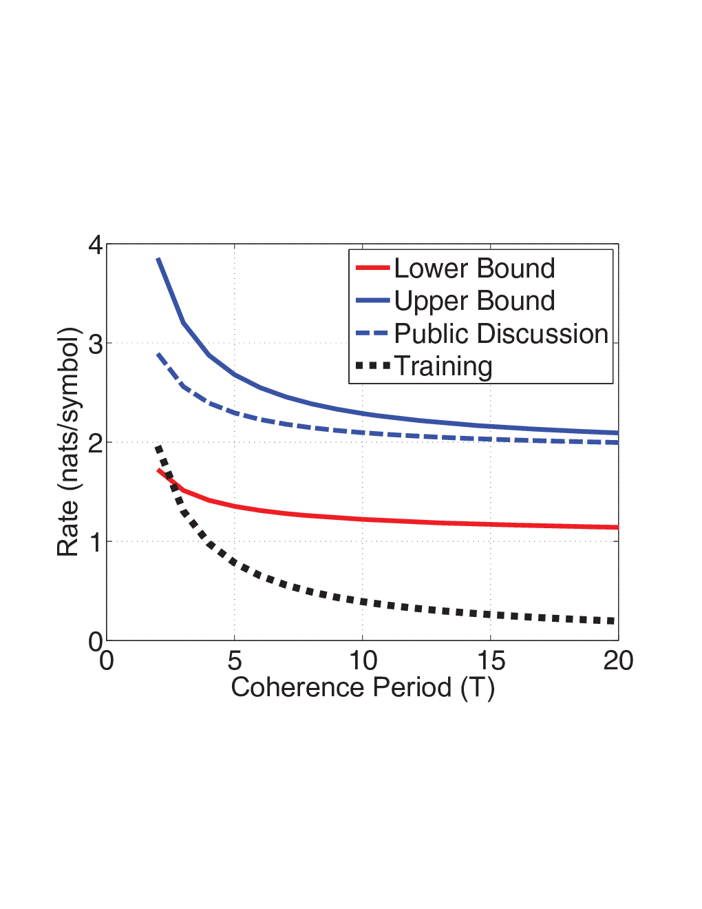
Fig. 5: Bounds on the SK capacity as a function of coherence period for SNR = 30dB.
Proposition 2

An achievable secret-key rate in the absence of public discussion for the two-way reciprocal fading channel is given by:

R−=1+ε1+ε2​{1T​RI​(ε1,P1)+T−1T​RII​(ε2,P2)}\displaystyle\!\!R^{-}=\frac{1}{\!\!1\!\!+\!\!\varepsilon_{1}\!\!+\!\!\varepsilon_{2}}\bigg\{\frac{1}{T}R_{\mathrm{I}}(\varepsilon_{1},P_{1})+\frac{T-1}{T}R_{\mathrm{II}}(\varepsilon_{2},P_{2})\bigg\} (26)

where P1P_{1} and P2P_{2} are non-negative and satisfy (9) and ε1\varepsilon_{1} and ε2\varepsilon_{2} are non-negative constants that will be specified in the sequel. The rate expressions RIR_{\mathrm{I}} and RIIR_{\mathrm{II}} are as follows.

RI​(ε1,P1)={−2​log⁡(1−α2​ρ21+Q1α)+log⁡(1−α2​ρ2(1+Q1α)2)}R_{\mathrm{I}}(\varepsilon_{1},P_{1})=\\ \left\{\!\!-2\log\left(1-\frac{\alpha^{2}\rho^{2}}{1+\frac{Q_{1}}{\alpha}}\right)\!\!+\!\!\log\left(1-\frac{\alpha^{2}\rho^{2}}{\left(1+\frac{Q_{1}}{\alpha}\right)^{2}}\!\!\right)\right\} (27)

where α=P11+P1\alpha=\frac{P_{1}}{1+P_{1}} and Q1Q_{1} satisfies

log⁡(1+α⁡(1−α2​ρ2)Q1)≤ε1​T​RNC​(P).\displaystyle\log\left(1+\frac{\alpha(1-\alpha^{2}\rho^{2})}{Q_{1}}\right)\leq\varepsilon_{1}TR_{\mathrm{NC}}(P). (28)

The expression for RIIR_{\mathrm{II}} satisfies

RII​(ε2,P2)\displaystyle R_{\mathrm{II}}(\varepsilon_{2},P_{2})\!\! ={RA​B−​(ε2,P2)+RB​A−​(ε2,P2)},\displaystyle=\!\!\bigg\{R_{AB}^{-}(\varepsilon_{2},P_{2})\!\!+\!\!R_{BA}^{-}(\varepsilon_{2},P_{2})\bigg\}, (29)
RA​B−​(ε2,P2)\displaystyle\!\!R_{AB}^{-}(\varepsilon_{2},P_{2})\!\! =E⁡[log⁡(1+P2​|𝘩A​B|2(1+Q2)​(1+P2​|𝘨A​E|2))]\displaystyle=\!\!E\left[\!\log\left(\!\!1+\!\!\frac{P_{2}|{\mathssf{h}}_{AB}|^{2}}{(1+Q_{2})(1+P_{2}|{\mathssf{g}}_{AE}|^{2}\!)}\right)\!\right]
−log⁡(σA​B2​P21+Q2+1),\displaystyle\qquad-\log\left(\frac{\sigma_{AB}^{2}P_{2}}{1+Q_{2}}+1\right), (30)
RB​A−​(ε2,P2)\displaystyle\!\!R_{BA}^{-}\!(\varepsilon_{2},P_{2})\! =E⁡[log⁡(+P2​|𝘩B​A|2(1+Q2)​(1+P2​|𝘨B​E|2))]\displaystyle=\!\!E\left[\!\log\!\!\left(\!\!1\!\!+\!\!\frac{P_{2}|{\mathssf{h}}_{BA}|^{2}}{(1+Q_{2})(1+P_{2}|{\mathssf{g}}_{BE}|^{2})}\!\right)\!\right]
−log⁡(σB​A2​P21+Q2+1),\displaystyle\qquad-\log\left(\frac{\sigma_{BA}^{2}P_{2}}{1+Q_{2}}+1\right), (31)

where

σA​B2=σB​A2=1−α2Q1+α\displaystyle\sigma_{AB}^{2}=\sigma_{BA}^{2}=1-\frac{\alpha^{2}}{Q_{1}+\alpha} (32)

and Q2Q_{2} satisfies

log⁡(1+σA​B2​P2+1Q2)≤ε2​RNC​(P).\displaystyle\log\left(1+\frac{\sigma_{AB}^{2}P_{2}+1}{Q_{2}}\right)\leq\varepsilon_{2}R_{\mathrm{NC}}(P). (33)

□\hfill\Box

A proof of Prop. 2 appears in section V-H.

Remark 4

The rate achieved in Prop. 2 reduces to the rate achieved using public discussion in Prop. 1 when we take Q1=Q2=0{Q_{1}=Q_{2}=0}. In particular when Q1=0Q_{1}=0 note that the expression for RIR_{\mathrm{I}} in (27) immediately reduces to (10). Furthermore (32) reduces to

σA​B2=σB​A2=11+P1.\displaystyle\sigma_{AB}^{2}=\sigma_{BA}^{2}=\frac{1}{1+P_{1}}. (34)

Substituting Q2=0,Q_{2}=0, and (34) in (30) and (31) we obtain (12) and (13) respectively. Thus the rate expressions in Prop. 2 are consistent with the expressions in Prop. 1 when quantization (c.f. (24) and (25)) is not introduced.

We also observe that the upper and lower bounds are close in the high signal-to-noise-ratio (SNR) regime.

Corollary 1

In the high SNR regime the upper and lower bounds satisfy the following relation:

limP→∞R+​(P)−RPD−​(P)=1T​γ\displaystyle\lim_{P\rightarrow\infty}R^{+}(P)-R^{-}_{\mathrm{PD}}(P)=\frac{1}{T}\gamma (35)
limP→∞R+​(P)−R−​(P)=1T​γ\displaystyle\lim_{P\rightarrow\infty}R^{+}(P)-R^{-}(P)=\frac{1}{T}\gamma (36)

where R+,R^{+}, RPD−R^{-}_{\mathrm{PD}} and R−R^{-} are given by (3), (10) and (26) respectively and

γ≜E⁡[log⁡(1+|𝘩A​B|2|𝘨A​E|2)]+E⁡[log⁡(1+|𝘩B​A|2|𝘨B​E|2)]\displaystyle\gamma\triangleq\!\!E\left[\log\left(1+\frac{|{\mathssf{h}}_{AB}|^{2}}{|{\mathssf{g}}_{AE}|^{2}}\right)\right]\!\!+\!\!E\left[\log\left(1+\frac{|{\mathssf{h}}_{BA}|^{2}}{|{\mathssf{g}}_{BE}|^{2}}\right)\right] (37)

is a constant that only depends on the distributions p⁡(𝘩A​B)​p​(𝘨A​E)p({\mathssf{h}}_{AB})p({\mathssf{g}}_{AE}) and p⁡(𝘩B​A)​p​(𝘨B​E)p({\mathssf{h}}_{BA})p({\mathssf{g}}_{BE}).

A proof of Corollary 1 appears in section VI.

Numerical Comparison:

Fig. 5 shows the bounds on secret-key capacity as a function of SNR when the coherence period T=10T=10. Fig. 5 shows the bounds as a function of the coherence period TT when SNR = 3535 dB. In Fig. 5 we fix the correlation coefficient in uplink and downlink gains to ρ=0.95\rho=0.95 while in Fig. 5 it is fixed to ρ=0.99\rho=0.99.

We make several observations in these plots. The lowermost plot in both figures corresponds to the best rate any training based scheme can achieve i.e.,

Rtraining=−1T​log⁡(1−ρ2)\displaystyle R_{\mathrm{training}}=-\frac{1}{T}\log(1-\rho^{2}) (38)

In computing (38) we assume that the legitimate receivers have a genie-aided side information of the respective channel gains and furthermore no overhead arising from the transmission of public messages is considered. In Fig. 5 this rate is SNR independent and in Fig. 5 it decreases to zero as 1T\frac{1}{T}.

The upper-most plot in Fig. 5 and Fig. 5 is the upper bound on the secret-key agreement capacity for any scheme. We note that for small values of TT the contribution from channel-reciprocity term in (3) is dominant. As TT increases the contribution of this term diminishes and the contribution from the communication channel increases (c.f. (3)).

The remaining two plots are the lower bounds with and without public discussion. The lower bound with public discussion does not involve the overhead of transmitting a public message. For sufficiently high SNR, it approaches the upper bound. The lower bound without public discussion does not come close to the upper in the SNR range of interest. Nevertheless it achieves a much higher rate than the training based schemes.

III Proof of Theorem 1

In this section we provide a proof of Theorem 1. We assume that the communication is over a total of KK coherence blocks and let N=T⋅KN=T\cdot K denote the total number of channel uses. Thus the channel state-sequences are of length KK whereas the channel input and output sequences are of length NN. We use the notation 𝘩A​BK{{\mathssf{h}}}_{AB}^{K} to denote the channel state sequence of length KK and the notation 𝘹AN{\mathssf{x}}_{A}^{N} to denote a channel input sequence of length NN. For the eavesdropper, we use the the notation 𝘇N≜(𝘻A​EN,𝘻B​EN){\mathbsf{z}}^{N}\triangleq({\mathssf{z}}_{AE}^{N},{\mathssf{z}}_{BE}^{N}) and 𝗴K≜(𝘨A​EK,𝘨B​EK){{{\mathbsf{g}}}}^{K}\triangleq({{\mathssf{g}}}_{AE}^{K},{{\mathssf{g}}}_{BE}^{K}).

From the Fano’s inequality and the secrecy constraint we have that

N​R\displaystyle NR ≤I⁡(𝘬A,𝘬B)−I⁡(𝘬A,𝘇N,𝗴K)+2​n​εn\displaystyle\leq I({\mathssf{k}}_{A};{\mathssf{k}}_{B})-I({\mathssf{k}}_{A};{\mathbsf{z}}^{N},{{{\mathbsf{g}}}}^{K})+2n\varepsilon_{n} (39)
≤I(𝘬A;𝘬B|𝘇N,𝗴K)+2nεn\displaystyle\leq I({\mathssf{k}}_{A};{\mathssf{k}}_{B}|{\mathbsf{z}}^{N},{{{\mathbsf{g}}}}^{K})+2n\varepsilon_{n} (40)

where εn→0\varepsilon_{n}\rightarrow 0 as n→∞n\rightarrow\infty. In the following steps the term εn\varepsilon_{n} will be suppressed. Since 𝘬A=fA​(𝘮A,𝘺AN){\mathssf{k}}_{A}=f_{A}({\mathssf{m}}_{A},{\mathssf{y}}_{A}^{N}) and 𝘬B=fB​(𝘮B,𝘺BN),{\mathssf{k}}_{B}=f_{B}({\mathssf{m}}_{B},{\mathssf{y}}_{B}^{N}), using the data-processing inequality and the chain rule of mutual information, we have:

NR≤I(𝘮A,𝘩B​AK,𝘺AN;𝘮B,𝘩A​BK,𝘺BN|𝘇N,𝗴K)\displaystyle NR\leq I({\mathssf{m}}_{A},{{\mathssf{h}}}_{BA}^{K},{\mathssf{y}}_{A}^{N};{\mathssf{m}}_{B},{{\mathssf{h}}}_{AB}^{K},{\mathssf{y}}_{B}^{N}|{\mathbsf{z}}^{N},{{{\mathbsf{g}}}}^{K})
=I(𝘮A,𝘩B​AK,𝘺AN;𝘮B,𝘩A​BK,𝘺BN−1|𝘇N,𝗴K)+\displaystyle=I({\mathssf{m}}_{A},{{\mathssf{h}}}_{BA}^{K},{\mathssf{y}}_{A}^{N};{\mathssf{m}}_{B},{{\mathssf{h}}}_{AB}^{K},{\mathssf{y}}_{B}^{N-1}|{\mathbsf{z}}^{N},{{{\mathbsf{g}}}}^{K})+
I(𝘮A,𝘩B​AK,𝘺AN;𝘺B(N)|𝘇N,𝗴K,𝘮B,𝘩A​BK,𝘺BN−1)\displaystyle I({\mathssf{m}}_{A},{{\mathssf{h}}}_{BA}^{K},{\mathssf{y}}_{A}^{N};{\mathssf{y}}_{B}(N)|{\mathbsf{z}}^{N},{{{\mathbsf{g}}}}^{K},{\mathssf{m}}_{B},{{\mathssf{h}}}_{AB}^{K},{\mathssf{y}}_{B}^{N-1})
=I(𝘮A,𝘩B​AK,𝘺AN−1;𝘮B,𝘩A​BK,𝘺BN−1|𝘇N,𝗴K)+\displaystyle=I({\mathssf{m}}_{A},{{\mathssf{h}}}_{BA}^{K},{\mathssf{y}}_{A}^{N-1};{\mathssf{m}}_{B},{{\mathssf{h}}}_{AB}^{K},{\mathssf{y}}_{B}^{N-1}|{\mathbsf{z}}^{N},{{{\mathbsf{g}}}}^{K})+
I(𝘺A(N);𝘮B,𝘩A​BK,𝘺BN−1|𝘇N,𝗴K,𝘮A,𝘩B​AK,𝘺AN−1)+\displaystyle I({\mathssf{y}}_{A}(N);{\mathssf{m}}_{B},{{\mathssf{h}}}_{AB}^{K},{\mathssf{y}}_{B}^{N-1}|{\mathbsf{z}}^{N},{{{\mathbsf{g}}}}^{K},{\mathssf{m}}_{A},{{\mathssf{h}}}_{BA}^{K},{\mathssf{y}}_{A}^{N-1})+
I(𝘮A,𝘩B​AK,𝘺AN−1;𝘺B(N)|𝘇N,𝗴K,𝘮B,𝘩A​BK,𝘺BN−1)+\displaystyle I({\mathssf{m}}_{A},{{\mathssf{h}}}_{BA}^{K},{\mathssf{y}}_{A}^{N-1};{\mathssf{y}}_{B}(N)|{\mathbsf{z}}^{N},{{{\mathbsf{g}}}}^{K},{\mathssf{m}}_{B},{{\mathssf{h}}}_{AB}^{K},{\mathssf{y}}_{B}^{N-1})+
I(𝘺A(N);𝘺B(N)|𝘇N,𝗴K,𝘮B,𝘩A​BK,𝘺BN−1,𝘮A,𝘩B​AK,𝘺AN−1).\displaystyle{{I({\mathssf{y}}_{A}(N);{\mathssf{y}}_{B}(N)|{\mathbsf{z}}^{N}\!\!,{{{\mathbsf{g}}}}^{K},\!\!{\mathssf{m}}_{B},{{\mathssf{h}}}_{AB}^{K},{\mathssf{y}}_{B}^{N-1},\!\!{\mathssf{m}}_{A},{{\mathssf{h}}}_{BA}^{K},\!\!{\mathssf{y}}_{A}^{N-1})}}. (41)
I(𝘮A,𝘩B​AK,𝘺AN−1;𝘮B,𝘩A​BK,𝘺BN−1|𝘇N,𝗴K)\displaystyle I({\mathssf{m}}_{A},{{\mathssf{h}}}_{BA}^{K},{\mathssf{y}}_{A}^{N-1};{\mathssf{m}}_{B},{{\mathssf{h}}}_{AB}^{K},{\mathssf{y}}_{B}^{N-1}|{\mathbsf{z}}^{N},{\mathbsf{g}}^{K}) (42)
≤I(𝘮A,𝘩B​AK,𝘺AN−1,𝘻A​E(N);𝘮B,𝘩A​BK,𝘺BN−1,𝘻B​E(N)|𝘇N−1,𝗴K)\displaystyle\leq I({\mathssf{m}}_{A},{{\mathssf{h}}}_{BA}^{K},{\mathssf{y}}_{A}^{N-1},{\mathssf{z}}_{AE}(N);{\mathssf{m}}_{B},{{\mathssf{h}}}_{AB}^{K},{\mathssf{y}}_{B}^{N-1},{\mathssf{z}}_{BE}(N)|{\mathbsf{z}}^{N-1},{{{\mathbsf{g}}}}^{K}) (43)
=I(𝘮A,𝘩B​AK,𝘺AN−1;𝘮B,𝘩A​BK,𝘺BN−1,𝘻B​E(N)|𝘇N−1,𝗴K)\displaystyle=I({\mathssf{m}}_{A},{{\mathssf{h}}}_{BA}^{K},{\mathssf{y}}_{A}^{N-1};{\mathssf{m}}_{B},{{\mathssf{h}}}_{AB}^{K},{\mathssf{y}}_{B}^{N-1},{\mathssf{z}}_{BE}(N)|{\mathbsf{z}}^{N-1},{{{\mathbsf{g}}}}^{K})
+I(𝘻A​E(N);𝘮B,𝘩A​BK,𝘺BN−1,𝘻B​E(N)|𝘇N−1,𝗴K,𝘮A,𝘩B​AK,𝘺AN−1)\displaystyle\qquad+I({\mathssf{z}}_{AE}(N);{\mathssf{m}}_{B},{{\mathssf{h}}}_{AB}^{K},{\mathssf{y}}_{B}^{N-1},{\mathssf{z}}_{BE}(N)|{\mathbsf{z}}^{N-1},{{{\mathbsf{g}}}}^{K},{\mathssf{m}}_{A},{{\mathssf{h}}}_{BA}^{K},{\mathssf{y}}_{A}^{N-1}) (44)
=I(𝘮A,𝘩B​AK,𝘺AN−1;𝘮B,𝘩A​BK,𝘺BN−1,𝘻B​E(N)|𝘇N−1,𝗴K)\displaystyle=I({\mathssf{m}}_{A},{{\mathssf{h}}}_{BA}^{K},{\mathssf{y}}_{A}^{N-1};{\mathssf{m}}_{B},{{\mathssf{h}}}_{AB}^{K},{\mathssf{y}}_{B}^{N-1},{\mathssf{z}}_{BE}(N)|{\mathbsf{z}}^{N-1},{{{\mathbsf{g}}}}^{K}) (45)
=I(𝘮A,𝘩B​AK,𝘺AN−1;𝘮B,𝘩A​BK,𝘺BN−1|𝘇N−1,𝗴K)+I(𝘮A,𝘩B​AK,𝘺AN−1;𝘻B​E(N)|𝘇N−1,𝗴K,𝘮B,𝘩A​BK,𝘺BN−1)\displaystyle=I({\mathssf{m}}_{A},{{\mathssf{h}}}_{BA}^{K},{\mathssf{y}}_{A}^{N-1};{\mathssf{m}}_{B},{{\mathssf{h}}}_{AB}^{K},{\mathssf{y}}_{B}^{N-1}|{\mathbsf{z}}^{N-1},{{{\mathbsf{g}}}}^{K})+I({\mathssf{m}}_{A},{{\mathssf{h}}}_{BA}^{K},{\mathssf{y}}_{A}^{N-1};{\mathssf{z}}_{BE}(N)|{\mathbsf{z}}^{N-1},{{{\mathbsf{g}}}}^{K},{\mathssf{m}}_{B},{{\mathssf{h}}}_{AB}^{K},{\mathssf{y}}_{B}^{N-1}) (46)
=I(𝘮A,𝘩B​AK,𝘺AN−1;𝘮B,𝘩A​BK,𝘺BN−1|𝘇N−1,𝗴K)\displaystyle=I({\mathssf{m}}_{A},{{\mathssf{h}}}_{BA}^{K},{\mathssf{y}}_{A}^{N-1};{\mathssf{m}}_{B},{{\mathssf{h}}}_{AB}^{K},{\mathssf{y}}_{B}^{N-1}|{\mathbsf{z}}^{N-1},{{{\mathbsf{g}}}}^{K}) (47)

We bound each of the four terms in (41). We show that the following condition holds

I(𝘮A,𝘩B​AK,𝘺AN−1;𝘮B,𝘩A​BK,𝘺BN−1|𝘇N,𝗴K)\displaystyle I({\mathssf{m}}_{A},{{\mathssf{h}}}_{BA}^{K},{\mathssf{y}}_{A}^{N-1};{\mathssf{m}}_{B},{{\mathssf{h}}}_{AB}^{K},{\mathssf{y}}_{B}^{N-1}|{\mathbsf{z}}^{N},{{{\mathbsf{g}}}}^{K})
≤I(𝘮A,𝘩B​AK,𝘺AN−1;𝘮B,𝘩A​BK,𝘺BN−1|𝘇N−1,𝗴K)\displaystyle\leq I({\mathssf{m}}_{A},{{\mathssf{h}}}_{BA}^{K},{\mathssf{y}}_{A}^{N-1};{\mathssf{m}}_{B},{{\mathssf{h}}}_{AB}^{K},{\mathssf{y}}_{B}^{N-1}|{\mathbsf{z}}^{N-1},{{{\mathbsf{g}}}}^{K}) (48)

in the steps between (42) and (47) on the top of next page. Note that (45) follows from the fact that 𝘹A​(N){\mathssf{x}}_{A}(N) is a function of (𝘮A,𝘺AN−1)({\mathssf{m}}_{A},{\mathssf{y}}_{A}^{N-1}) and furthermore 𝘻A​E​(N){\mathssf{z}}_{AE}(N) is independent of all other random variables given (𝘹A​(N),𝘨A​E​(N))({\mathssf{x}}_{A}(N),{\mathssf{g}}_{AE}(N)) (c.f. (2)). Eq. (47) similarly follows because 𝘹B​(N){\mathssf{x}}_{B}(N) is a function of (𝘮B,𝘺BN−1)({\mathssf{m}}_{B},{\mathssf{y}}_{B}^{N-1}) and furthermore 𝘻B​E​(N){\mathssf{z}}_{BE}(N) is independent of all other random variables given (𝘹B​(N),𝘨B​E​(N))({\mathssf{x}}_{B}(N),{\mathssf{g}}_{BE}(N)).

Furthermore, since (𝘺A​(N),𝘻B​E​(N))({\mathssf{y}}_{A}(N),{\mathssf{z}}_{BE}(N)) are independent of all other random variables given (𝘹B​(N),𝘩B​A​(N),𝘨B​E​(N))({\mathssf{x}}_{B}(N),{\mathssf{h}}_{BA}(N),{\mathssf{g}}_{BE}(N)) we can show that

I(𝘺A(N);𝘮B,𝘩A​BK,𝘺BN−1|𝘇N,𝗴K,𝘮A,𝘩B​AK,𝘺AN−1)\displaystyle I({\mathssf{y}}_{A}(N);{\mathssf{m}}_{B},{{\mathssf{h}}}_{AB}^{K},{\mathssf{y}}_{B}^{N-1}|{\mathbsf{z}}^{N},{{{\mathbsf{g}}}}^{K},{\mathssf{m}}_{A},{{\mathssf{h}}}_{BA}^{K},{\mathssf{y}}_{A}^{N-1})
≤I(𝘺A(N);𝘹B(N)|𝘻B​E(N),𝘨B​E(N),𝘩B​A(N)).\displaystyle\leq I({\mathssf{y}}_{A}(N);{\mathssf{x}}_{B}(N)|{\mathssf{z}}_{BE}(N),{\mathssf{g}}_{BE}(N),{\mathssf{h}}_{BA}(N)). (49)

and likewise

I(𝘮A,𝘩B​AK,𝘺AN−1;𝘺B(N)|𝘇N,𝗴K,𝘮B,𝘩A​BK,𝘺BN−1)\displaystyle I({\mathssf{m}}_{A},{{\mathssf{h}}}_{BA}^{K},{\mathssf{y}}_{A}^{N-1};{\mathssf{y}}_{B}(N)|{\mathbsf{z}}^{N},{{{\mathbsf{g}}}}^{K},{\mathssf{m}}_{B},{{\mathssf{h}}}_{AB}^{K},{\mathssf{y}}_{B}^{N-1})
≤I(𝘹A(N);𝘺B(N)|𝘻A​E(N),𝘩A​B(N),𝘨A​E(N)).\displaystyle\leq I({\mathssf{x}}_{A}(N);{\mathssf{y}}_{B}(N)|{\mathssf{z}}_{AE}(N),{\mathssf{h}}_{AB}(N),{\mathssf{g}}_{AE}(N)). (50)

Finally using the fact that 𝘹A​(N){\mathssf{x}}_{A}(N) and 𝘹B​(N){\mathssf{x}}_{B}(N) are functions of (𝘮A,𝘺B​AN−1)({\mathssf{m}}_{A},{\mathssf{y}}_{BA}^{N-1}) and (𝘮B,𝘺A​BN−1)({\mathssf{m}}_{B},{\mathssf{y}}_{AB}^{N-1}) respectively and the fact that 𝘺A​(N){\mathssf{y}}_{A}(N) is independent of all other random variables given (𝘹A​(N),𝘩A​B​(N))({\mathssf{x}}_{A}(N),{\mathssf{h}}_{AB}(N)) and similarly 𝘺B​(N){\mathssf{y}}_{B}(N) is independent of all other random variables given (𝘹B​(N),𝘩B​A​(N))({\mathssf{x}}_{B}(N),{\mathssf{h}}_{BA}(N)) we can show that

I(𝘺A(N);𝘺B(N)|𝘇N,𝗴K,𝘮B,𝘩A​BK,𝘺BN−1,𝘮A,𝘩B​AK,𝘺AN−1)\displaystyle I({\mathssf{y}}_{A}(N);{\mathssf{y}}_{B}(N)|{\mathbsf{z}}^{N}\!\!,{{{\mathbsf{g}}}}^{K},\!\!{\mathssf{m}}_{B},{{\mathssf{h}}}_{AB}^{K},{\mathssf{y}}_{B}^{N-1},\!\!{\mathssf{m}}_{A},{{\mathssf{h}}}_{BA}^{K},\!\!{\mathssf{y}}_{A}^{N-1})
=0.\displaystyle\qquad=0. (51)

Thus substituting (48), (49) and (50) into (41) we have that

N​R\displaystyle NR ≤I(𝘮A,𝘩B​AK,𝘺AN−1;𝘮B,𝘩A​BK,𝘺BN−1|𝘇N−1,𝗴K)\displaystyle\leq I({\mathssf{m}}_{A},{{\mathssf{h}}}_{BA}^{K},{\mathssf{y}}_{A}^{N-1};{\mathssf{m}}_{B},{{\mathssf{h}}}_{AB}^{K},{\mathssf{y}}_{B}^{N-1}|{\mathbsf{z}}^{N-1},{{{\mathbsf{g}}}}^{K})
+I(𝘺A(N);𝘹B(N)|𝘻B​E(N),𝘨B​E(N),𝘩B​A(N))\displaystyle+I({\mathssf{y}}_{A}(N);{\mathssf{x}}_{B}(N)|{\mathssf{z}}_{BE}(N),{\mathssf{g}}_{BE}(N),{\mathssf{h}}_{BA}(N))
+I(𝘹A(N);𝘺B(N)|𝘻A​E(N),𝘩A​B(N),𝘨A​E(N))\displaystyle+I({\mathssf{x}}_{A}(N);{\mathssf{y}}_{B}(N)|{\mathssf{z}}_{AE}(N),{\mathssf{h}}_{AB}(N),{\mathssf{g}}_{AE}(N)) (52)

Recursively applying the same steps we have that

N​R\displaystyle NR ≤I⁡(𝘮A,𝘩B​AK;𝘩A​BK,𝘮B|𝗴K)+\displaystyle\leq I({\mathssf{m}}_{A},{{\mathssf{h}}}_{BA}^{K};{{\mathssf{h}}}_{AB}^{K},{\mathssf{m}}_{B}|{{{\mathbsf{g}}}}^{K})+
∑i=1NI(𝘹B(i);𝘺A(i)|𝘻B​E(i),𝘨B​E(i),𝘩B​A(i))+\displaystyle\sum_{i=1}^{N}I({\mathssf{x}}_{B}(i);{\mathssf{y}}_{A}(i)|{\mathssf{z}}_{BE}(i),{\mathssf{g}}_{BE}(i),{\mathssf{h}}_{BA}(i))+
∑i=1NI(𝘹A(i);𝘺B(i)|𝘻A​E(i),𝘨A​E(i),𝘩A​B(i))\displaystyle\sum_{i=1}^{N}I({\mathssf{x}}_{A}(i);{\mathssf{y}}_{B}(i)|{\mathssf{z}}_{AE}(i),{\mathssf{g}}_{AE}(i),{\mathssf{h}}_{AB}(i)) (53)
=K​I​(𝘩B​A,𝘩A​B)+\displaystyle=KI({\mathssf{h}}_{BA};{\mathssf{h}}_{AB})+
∑i=1NI(𝘹B(i);𝘺A(i)|𝘻B​E(i),𝘨B​E(i),𝘩B​A(i))+\displaystyle\sum_{i=1}^{N}I({\mathssf{x}}_{B}(i);{\mathssf{y}}_{A}(i)|{\mathssf{z}}_{BE}(i),{\mathssf{g}}_{BE}(i),{\mathssf{h}}_{BA}(i))+
∑i=1NI(𝘹A(i);𝘺B(i)|𝘻A​E(i),𝘨A​E(i),𝘩A​B(i))\displaystyle\sum_{i=1}^{N}I({\mathssf{x}}_{A}(i);{\mathssf{y}}_{B}(i)|{\mathssf{z}}_{AE}(i),{\mathssf{g}}_{AE}(i),{\mathssf{h}}_{AB}(i)) (54)

where in (54) we use the fact that (𝘮A,𝘮B)({\mathssf{m}}_{A},{\mathssf{m}}_{B}) are mutually independent and independent of the channel gains and furthermore (𝘩A​BK,𝘩B​AK)({{\mathssf{h}}}_{AB}^{K},{{\mathssf{h}}}_{BA}^{K}) are independent of 𝗴K{{{\mathbsf{g}}}}^{K}. Finally to establish the upper bound (3) suppose that we assign a power Pi​(hA​B)P_{i}(h_{AB}) when the channel gain at time ii equals hA​Bh_{AB}. Using the fact that a Gaussian input distribution maximizes the conditional mutual information terms in (54) (see e.g., [41]) we have:

I(𝘹A(i);𝘺B(i)|𝘻A​E(i),𝘨A​E(i),𝘩A​B(i))\displaystyle I({\mathssf{x}}_{A}(i);{\mathssf{y}}_{B}(i)|{\mathssf{z}}_{AE}(i),{\mathssf{g}}_{AE}(i),{\mathssf{h}}_{AB}(i))
≤E⁡[log⁡(1+Pi​(𝘩A​B)​|𝘩A​B|21+Pi​(𝘩A​B)​|𝘨A​E|2)].\displaystyle\leq E\left[\log\left(1+\frac{P_{i}({\mathssf{h}}_{AB})|{\mathssf{h}}_{AB}|^{2}}{1+P_{i}({\mathssf{h}}_{AB})|{\mathssf{g}}_{AE}|^{2}}\right)\right]. (55)

Thus we have that

∑i=1NI(𝘹A(i);𝘺B(i)|𝘻A​E(i),𝘨A​E(i),𝘩A​B(i))\displaystyle\sum_{i=1}^{N}I({\mathssf{x}}_{A}(i);{\mathssf{y}}_{B}(i)|{\mathssf{z}}_{AE}(i),{\mathssf{g}}_{AE}(i),{\mathssf{h}}_{AB}(i))
≤∑i=1NE⁡[log⁡(1+Pi​(𝘩A​B)​|𝘩A​B|21+Pi​(𝘩A​B)​|𝘨A​E|2)]\displaystyle\leq\sum_{i=1}^{N}E\left[\log\left(1+\frac{P_{i}({\mathssf{h}}_{AB})|{\mathssf{h}}_{AB}|^{2}}{1+P_{i}({\mathssf{h}}_{AB})|{\mathssf{g}}_{AE}|^{2}}\right)\right] (56)
=E⁡[∑i=1Nlog⁡(1+Pi​(𝘩A​B)​|𝘩A​B|21+Pi​(𝘩A​B)​|𝘨A​E|2)]\displaystyle=E\left[\sum_{i=1}^{N}\log\left(1+\frac{P_{i}({\mathssf{h}}_{AB})|{\mathssf{h}}_{AB}|^{2}}{1+P_{i}({\mathssf{h}}_{AB})|{\mathssf{g}}_{AE}|^{2}}\right)\right] (57)
≤N​E​[log⁡(1+1N​∑i=1NPi​(𝘩A​B)​|𝘩A​B|21+1N​∑i=1NPi​(𝘩A​B)​|𝘨A​E|2)]\displaystyle\leq NE\left[\log\left(1+\frac{\frac{1}{N}\sum_{i=1}^{N}P_{i}({\mathssf{h}}_{AB})|{\mathssf{h}}_{AB}|^{2}}{1+\frac{1}{N}\sum_{i=1}^{N}P_{i}({\mathssf{h}}_{AB})|{\mathssf{g}}_{AE}|^{2}}\right)\right] (58)
=N​E​[log⁡(1+P⁡(𝘩A​B)​|𝘩A​B|21+P⁡(𝘩A​B)​|𝘨A​E|2)],\displaystyle=NE\left[\log\left(1+\frac{P({\mathssf{h}}_{AB})|{\mathssf{h}}_{AB}|^{2}}{1+P({\mathssf{h}}_{AB})|{\mathssf{g}}_{AE}|^{2}}\right)\right], (59)
=NI(𝘹A;𝘺B|𝘻A​E,𝘨A​E,𝘩A​B)\displaystyle=NI({\mathssf{x}}_{A};{\mathssf{y}}_{B}|{\mathssf{z}}_{AE},{\mathssf{g}}_{AE},{\mathssf{h}}_{AB}) (60)

where P⁡(𝘩A​B)≜1N​∑i=1NPi​(𝘩A​B)P({\mathssf{h}}_{AB})\triangleq\frac{1}{N}\sum_{i=1}^{N}P_{i}({\mathssf{h}}_{AB}) is the average power allocated when the fading state equals 𝘩A​B{\mathssf{h}}_{AB} and (58) uses the fact that the function f⁡(x)=log⁡(1+a​x1+b​x)f(x)=\log\left(1+\frac{ax}{1+bx}\right) is a concave function in xx and hence Jensen’s inequality applies. Also note that

E⁡[P⁡(𝘩A​B)]\displaystyle E[P({\mathssf{h}}_{AB})] =E⁡[1N​∑i=1NPi​(𝘩A​B)]\displaystyle=E\left[\frac{1}{N}\sum_{i=1}^{N}P_{i}({\mathssf{h}}_{AB})\right] (61)
=1N​∑i=1NE⁡[Pi​(𝘩A​B)]\displaystyle=\frac{1}{N}\sum_{i=1}^{N}E[P_{i}({\mathssf{h}}_{AB})] (62)
≤1N​∑i=1NPi≤P.\displaystyle\leq\frac{1}{N}\sum_{i=1}^{N}P_{i}\leq P. (63)

In a similar fashion we can show that

∑i=1NI(𝘹B(i);𝘺A(i)|𝘻B​E(i),𝘨B​E(i),𝘩B​A(i))\displaystyle\sum_{i=1}^{N}I({\mathssf{x}}_{B}(i);{\mathssf{y}}_{A}(i)|{\mathssf{z}}_{BE}(i),{\mathssf{g}}_{BE}(i),{\mathssf{h}}_{BA}(i))
≤N​E​[log⁡(1+P⁡(𝘩B​A)​|𝘩B​A|21+P⁡(𝘩B​A)​|𝘨B​E|2)].\displaystyle\leq NE\left[\log\left(1+\frac{P({\mathssf{h}}_{BA})|{\mathssf{h}}_{BA}|^{2}}{1+P({\mathssf{h}}_{BA})|{\mathssf{g}}_{BE}|^{2}}\right)\right]. (64)
=NI(𝘹B;𝘺A|𝘻B​E,𝘨B​E,𝘩B​A)\displaystyle=NI({\mathssf{x}}_{B};{\mathssf{y}}_{A}|{\mathssf{z}}_{BE},{\mathssf{g}}_{BE},{\mathssf{h}}_{BA}) (65)

The upper bound (3) follows by substituting in (60) and (65) into (54). This completes the proof of Theorem 1.

IV Proof of Theorem 2

We sketch the coding scheme associated with Theorem 2, where we assume the availability of a public discussion channel. In our proof we assume that the channel input and output symbols as well as the fading gains are discrete valued. We do not address the discretization of these random variables in this section; it will be addressed in the proof of Theorem 3, when we do not assume the availability of a discussion channel.

IV-A Generation of Correlated Source Sequences

In each coherence block we reserve the first symbol for transmission of a pilot symbol

𝘹A​(i​T+1)=𝘹B​(i​T+1)=P1,i=0,…,NT−1.{\mathssf{x}}_{A}(iT+1)={\mathssf{x}}_{B}(iT+1)=\sqrt{P_{1}},\\ i=0,\ldots,\frac{N}{T}-1. (66)

and the remainder of the symbols for transmission of i.i.d. random variables i.e.,

𝘹A(t)∼p𝘹A(⋅),𝘹B(t)∼p𝘹B(⋅),∀t∈[1,N],t≠iT+1.{\mathssf{x}}_{A}(t)\sim p_{{\mathssf{x}}_{A}}(\cdot),{\mathssf{x}}_{B}(t)\sim p_{{\mathssf{x}}_{B}}(\cdot),\forall t\in[1,N],t\neq iT+1. (67)

The legitimate receivers BB and AA use the corresponding output symbols 𝘺B​(i​T+1){\mathssf{y}}_{B}(iT+1) and 𝘺A​(i​T+1){\mathssf{y}}_{A}(iT+1) for estimating the underlying channel gains 𝘩^A​B​(i+1)\hat{{\mathssf{h}}}_{AB}(i+1) and 𝘩^B​A​(i+1)\hat{{\mathssf{h}}}_{BA}(i+1) in (5) and (6) respectively.

We use the bold-font notation 𝘅¯A​(t)\bar{{\mathbsf{x}}}_{A}(t) to denote the sequence of T−1{T-1} i.i.d. symbols transmitted in coherence block tt. and let 𝘆¯B​(t)\bar{{\mathbsf{y}}}_{B}(t) denote the corresponding output symbol vector in block tt. The source sequences at the terminals at the end of KK coherence blocks are indicated in Table I.

IV-B Information Reconciliation

Terminals AA and BB exchange public messages over the discussion channel to agree on identical sequence pair (𝘩^A​BK,𝘩^B​AK,𝘆¯A​BK,𝘆¯B​AK)(\hat{{\mathssf{h}}}_{AB}^{K},\hat{{\mathssf{h}}}_{BA}^{K},\bar{{\mathbsf{y}}}_{AB}^{K},\bar{{\mathbsf{y}}}_{BA}^{K}). The public messages transmitted are as follows (i) Terminal AA bins the sequences {𝘩^B​AK}\{\hat{{\mathssf{h}}}_{BA}^{K}\} into 2K⁡(H⁡(𝘩^B​A|𝘩^A​B)+ε)2^{K(H(\hat{{\mathssf{h}}}_{BA}|\hat{{\mathssf{h}}}_{AB})+\varepsilon)} bins and transmits the associated bin index ϕA\phi_{A} over the discussion channel. (ii) Terminal BB bins the sequences {𝘩^A​BK}\{\hat{{\mathssf{h}}}_{AB}^{K}\} into 2K⁡(H⁡(𝘩^A​B|𝘩^B​A)+ε)2^{K(H(\hat{{\mathssf{h}}}_{AB}|\hat{{\mathssf{h}}}_{BA})+\varepsilon)} bins and transmits the associated bin index ϕB\phi_{B} over the discussion channel. (iii) Terminal AA bins the sequences {𝘆¯AK}\{\bar{{\mathbsf{y}}}_{A}^{K}\} into 2K⁡(H⁡(𝘆¯A|𝘅¯B,𝘩^A​B,𝘩^B​A)+ε)2^{K(H(\bar{{\mathbsf{y}}}_{A}|\bar{{\mathbsf{x}}}_{B},\hat{{\mathssf{h}}}_{AB},\hat{{\mathssf{h}}}_{BA})+\varepsilon)} and transmits the associated bin index ψA\psi_{A} over the discussion channel. (iv) Terminal BB bins the sequence {𝘆¯BK}\{\bar{{\mathbsf{y}}}_{B}^{K}\} into 2K⁡(H⁡(𝘆¯B|𝘅¯A,𝘩^A​B,𝘩^B​A)+ε)2^{K(H(\bar{{\mathbsf{y}}}_{B}|\bar{{\mathbsf{x}}}_{A},\hat{{\mathssf{h}}}_{AB},\hat{{\mathssf{h}}}_{BA})+\varepsilon)} and transmits the associated bin index ψB\psi_{B} over the discussion channel.

Using standard arguments (see e.g., [42, Chap. 10]) Terminal AA can reconstruct the sequence pair (𝘩^A​BK,𝘆¯BK)(\hat{{\mathssf{h}}}_{AB}^{K},\bar{{\mathbsf{y}}}_{B}^{K}) (with high probability) given the messages (ϕB,ψB)(\phi_{B},\psi_{B}) and its side information (𝘩^B​AK,𝘅¯AK)(\hat{{\mathssf{h}}}_{BA}^{K},\bar{{\mathbsf{x}}}_{A}^{K}). Terminal BB can reconstruct the sequence pair (𝘩^B​AK,𝘆¯AK)(\hat{{\mathssf{h}}}_{BA}^{K},\bar{{\mathbsf{y}}}_{A}^{K}) (with high probability) given the messages (ϕA,ψA)(\phi_{A},\psi_{A}) and its side information sequence (𝘩^A​BK,𝘅¯BK)(\hat{{\mathssf{h}}}_{AB}^{K},\bar{{\mathbsf{x}}}_{B}^{K}). Thus at the end of this phase both terminals have access to the common sequence pair (𝘆¯AK,𝘆¯BK,𝘩^A​BK,𝘩^B​AK)(\bar{{\mathbsf{y}}}_{A}^{K},\bar{{\mathbsf{y}}}_{B}^{K},\hat{{\mathssf{h}}}_{AB}^{K},\hat{{\mathssf{h}}}_{BA}^{K}). The eavesdropper has access to (𝘇¯K,𝗴K,ϕA,ϕB,ψA,ψB)(\bar{{\mathbsf{z}}}^{K},{\mathbsf{g}}^{K},\phi_{A},\phi_{B},\psi_{A},\psi_{B}).

IV-C Equivocation Analysis

We lower bound the equivocation at the eavesdropper as follows:

H(𝘆¯AK,𝘆¯BK,𝘩^A​BK,𝘩^B​AK|𝘇¯K,𝗴K,ϕA,ϕB,ψA,ψB)\displaystyle\quad H(\bar{{\mathbsf{y}}}_{A}^{K},\bar{{\mathbsf{y}}}_{B}^{K},\hat{{\mathssf{h}}}_{AB}^{K},\hat{{\mathssf{h}}}_{BA}^{K}|\bar{{\mathbsf{z}}}^{K},{\mathbsf{g}}^{K},\phi_{A},\phi_{B},\psi_{A},\psi_{B})
=H(𝘆¯AK,𝘆¯BK,𝘩^A​BK,𝘩^B​AK|𝘇¯K,𝗴K)−H(ϕA)−H(ϕB)\displaystyle=H(\bar{{\mathbsf{y}}}_{A}^{K},\bar{{\mathbsf{y}}}_{B}^{K},\hat{{\mathssf{h}}}_{AB}^{K},\hat{{\mathssf{h}}}_{BA}^{K}|\bar{{\mathbsf{z}}}^{K},{\mathbsf{g}}^{K})-H(\phi_{A})-H(\phi_{B})
−H⁡(ψA)−H⁡(ψB)\displaystyle\qquad-H(\psi_{A})-H(\psi_{B})
=H(𝘩^A​BK,𝘩^B​AK)+H(𝘆¯AK,𝘆¯BK|𝘇¯K,𝗴K,𝘩^A​BK,𝘩^B​AK)\displaystyle=H(\hat{{\mathssf{h}}}_{AB}^{K},\hat{{\mathssf{h}}}_{BA}^{K})+H(\bar{{\mathbsf{y}}}_{A}^{K},\bar{{\mathbsf{y}}}_{B}^{K}|\bar{{\mathbsf{z}}}^{K},{\mathbsf{g}}^{K},\hat{{\mathssf{h}}}_{AB}^{K},\hat{{\mathssf{h}}}_{BA}^{K})
−H⁡(ϕA)−H⁡(ϕB)−H⁡(ψA)−H⁡(ψB)\displaystyle\qquad-H(\phi_{A})-H(\phi_{B})-H(\psi_{A})-H(\psi_{B}) (68)
≥H(𝘩^A​BK,𝘩^B​AK)+H(𝘆¯AK,𝘆¯BK|𝘇¯K,𝗴K,𝘩A​BK,𝘩B​AK)\displaystyle\geq H(\hat{{\mathssf{h}}}_{AB}^{K},\hat{{\mathssf{h}}}_{BA}^{K})+H(\bar{{\mathbsf{y}}}_{A}^{K},\bar{{\mathbsf{y}}}_{B}^{K}|\bar{{\mathbsf{z}}}^{K},{\mathbsf{g}}^{K},{\mathssf{h}}_{AB}^{K},{\mathssf{h}}_{BA}^{K})
−H⁡(ϕA)−H⁡(ϕB)−H⁡(ψA)−H⁡(ψB)\displaystyle\qquad-H(\phi_{A})-H(\phi_{B})-H(\psi_{A})-H(\psi_{B}) (69)
=H⁡(𝘩^A​BK,𝘩^B​AK)+H⁡(𝘆¯AK|𝘇¯BK,𝘨B​EK,𝘩B​AK)\displaystyle=\!\!H(\hat{{\mathssf{h}}}_{AB}^{K},\hat{{\mathssf{h}}}_{BA}^{K})\!\!+\!\!H(\bar{{\mathbsf{y}}}_{A}^{K}|\bar{{\mathbsf{z}}}_{B}^{K},{\mathssf{g}}_{BE}^{K},{\mathssf{h}}_{BA}^{K})
+H⁡(𝘆¯BK|𝘇¯AK,𝘨A​EK,𝘩A​BK)\displaystyle\qquad+\!\!H(\bar{{\mathbsf{y}}}_{B}^{K}|\bar{{\mathbsf{z}}}_{A}^{K},{\mathssf{g}}_{AE}^{K},{\mathssf{h}}_{AB}^{K})
−H⁡(ϕA)−H⁡(ϕB)−H⁡(ψA)−H⁡(ψB)\displaystyle\qquad-H(\phi_{A})-H(\phi_{B})-H(\psi_{A})-H(\psi_{B}) (70)
=K​H​(𝘩^A​B,𝘩^B​A)+K​H​(𝘆¯A|𝘇¯B,𝘨B​E,𝘩B​A)\displaystyle=KH(\hat{{\mathssf{h}}}_{AB},\hat{{\mathssf{h}}}_{BA})+KH(\bar{{\mathbsf{y}}}_{A}|\bar{{\mathbsf{z}}}_{B},{\mathssf{g}}_{BE},{\mathssf{h}}_{BA})
+K​H​(𝘆¯B|𝘇¯A,𝘨A​E,𝘩A​B)\displaystyle\qquad+KH(\bar{{\mathbsf{y}}}_{B}|\bar{{\mathbsf{z}}}_{A},{\mathssf{g}}_{AE},{\mathssf{h}}_{AB})
−H⁡(ϕA)−H⁡(ϕB)−H⁡(ψA)−H⁡(ψB)\displaystyle\qquad-H(\phi_{A})-H(\phi_{B})-H(\psi_{A})-H(\psi_{B}) (71)

where we use the chain rule of entropy and the fact that (𝘩^A​BK,𝘩^B​AK)(\hat{{\mathssf{h}}}_{AB}^{K},\hat{{\mathssf{h}}}_{BA}^{K}) is independent of (𝘇¯K,𝗴K)(\bar{{\mathbsf{z}}}^{K},{\mathbsf{g}}^{K}) in (68); in (69) we use the fact that conditioning reduces entropy as well as 𝘩^A​BK\hat{{\mathssf{h}}}_{AB}^{K} and 𝘩^B​AK\hat{{\mathssf{h}}}_{BA}^{K} are independent of the remaining variables gives 𝘩A​BK{\mathssf{h}}_{AB}^{K} and 𝘩B​AK{\mathssf{h}}_{BA}^{K} respectively; in (70) we use the fact that 𝘅¯AK\bar{{\mathbsf{x}}}_{A}^{K} and 𝘅¯BK\bar{{\mathbsf{x}}}_{B}^{K} are sampled independently and hence the following Markov conditions hold:

𝘆¯AK→(𝘇¯BK,𝘨B​EK,𝘩B​AK)→(𝘆¯BK,𝘨A​EK,𝘩A​BK)\displaystyle\bar{{\mathbsf{y}}}_{A}^{K}\rightarrow(\bar{{\mathbsf{z}}}_{B}^{K},{\mathssf{g}}_{BE}^{K},{\mathssf{h}}_{BA}^{K})\rightarrow(\bar{{\mathbsf{y}}}_{B}^{K},{\mathssf{g}}_{AE}^{K},{\mathssf{h}}_{AB}^{K}) (72)
𝘆¯BK→(𝘇¯AK,𝘨A​EK,𝘩A​BK)→(𝘆¯AK,𝘨B​EK,𝘩B​AK);\displaystyle\bar{{\mathbsf{y}}}_{B}^{K}\rightarrow(\bar{{\mathbsf{z}}}_{A}^{K},{\mathssf{g}}_{AE}^{K},{\mathssf{h}}_{AB}^{K})\rightarrow(\bar{{\mathbsf{y}}}_{A}^{K},{\mathssf{g}}_{BE}^{K},{\mathssf{h}}_{BA}^{K}); (73)

Eq. (71) follows from the fact that the sequence pair (𝘩A​BK,𝘩B​AK)({\mathssf{h}}_{AB}^{K},{\mathssf{h}}_{BA}^{K}) is sampled i.i.d. and furthermore 𝘅¯AK\bar{{\mathbsf{x}}}_{A}^{K} and 𝘅¯BK\bar{{\mathbsf{x}}}_{B}^{K} are also sampled i.i.d. Furthermore,

K​H​(𝘩A​B,𝘩B​A)−H⁡(ϕA)−H⁡(ϕB)\displaystyle KH({\mathssf{h}}_{AB},{\mathssf{h}}_{BA})-H(\phi_{A})-H(\phi_{B})
≥K​H​(𝘩^A​B,𝘩^B​A)−H⁡(𝘩^B​A|𝘩^A​B)−H⁡(𝘩^A​B|𝘩^B​A)−4​K​ε\displaystyle\geq KH(\hat{{\mathssf{h}}}_{AB},\hat{{\mathssf{h}}}_{BA})-H(\hat{{\mathssf{h}}}_{BA}|\hat{{\mathssf{h}}}_{AB})-H(\hat{{\mathssf{h}}}_{AB}|\hat{{\mathssf{h}}}_{BA})-4K\varepsilon (74)
=K​I​(𝘩^A​B,𝘩^B​A)−4​K​ε.\displaystyle=KI(\hat{{\mathssf{h}}}_{AB};\hat{{\mathssf{h}}}_{BA})-4K\varepsilon. (75)

Using the fact that 𝘅¯A\bar{{\mathbsf{x}}}_{A} is sampled i.i.d. in (77) and letting ε′=εT−1\varepsilon^{\prime}=\frac{\varepsilon}{T-1} we have

K​H​(𝘆¯A|𝘇¯B,𝘨B​E,𝘩B​A)−H⁡(ψA)\displaystyle KH(\bar{{\mathbsf{y}}}_{A}|\bar{{\mathbsf{z}}}_{B},{\mathssf{g}}_{BE},{\mathssf{h}}_{BA})-H(\psi_{A})
≥K​H​(𝘆¯A|𝘇¯B,𝘨B​E,𝘩B​A)−K​H​(𝘆¯A|𝘅¯B,𝘩^A​B,𝘩^B​A)−2​K​ε\displaystyle\geq KH(\bar{{\mathbsf{y}}}_{A}|\bar{{\mathbsf{z}}}_{B},{\mathssf{g}}_{BE},{\mathssf{h}}_{BA})-KH(\bar{{\mathbsf{y}}}_{A}|\bar{{\mathbsf{x}}}_{B},\hat{{\mathssf{h}}}_{AB},\hat{{\mathssf{h}}}_{BA})-2K\varepsilon (76)
=K⁡(T−1)​{H⁡(𝘺A|𝘻B,𝘨B​E,𝘩B​A)−H⁡(𝘺A|𝘹B,𝘩^A​B,𝘩^B​A)−2​ε′}\displaystyle\!\!=\!\!K(T-1)\left\{H({\mathssf{y}}_{A}|{\mathssf{z}}_{B},{\mathssf{g}}_{BE},{\mathssf{h}}_{BA})\!\!-\!\!H({\mathssf{y}}_{A}|{\mathssf{x}}_{B},\hat{{\mathssf{h}}}_{AB},\hat{{\mathssf{h}}}_{BA})\!\!-\!\!2\varepsilon^{\prime}\right\} (77)
=K⁡(T−1)​{I⁡(𝘺A,𝘹B,𝘩^A​B,𝘩^B​A)−I⁡(𝘺A,𝘻B,𝘨B​E,𝘩B​A)−2​ε′}.\displaystyle=K(T-1)\!\!\left\{I({\mathssf{y}}_{A};{\mathssf{x}}_{B},\hat{{\mathssf{h}}}_{AB},\hat{{\mathssf{h}}}_{BA})\!\!-\!\!I({\mathssf{y}}_{A};{\mathssf{z}}_{B},{\mathssf{g}}_{BE},{\mathssf{h}}_{BA})\!\!-\!\!2\varepsilon^{\prime}\right\}. (78)

In a similar fashion we can show that

K​H​(𝘆¯B|𝘇¯A,𝘨A​E,𝘩A​B)−H⁡(ψB)\displaystyle KH(\bar{{\mathbsf{y}}}_{B}|\bar{{\mathbsf{z}}}_{A},{\mathssf{g}}_{AE},{\mathssf{h}}_{AB})-H(\psi_{B})
≥K⁡(T−1)​{I⁡(𝘺B,𝘹A,𝘩^A​B,𝘩^B​A)−I⁡(𝘺B,𝘻A,𝘨A​E,𝘩A​B)−2​ε′}\displaystyle\geq K(T-1)\left\{I({\mathssf{y}}_{B};{\mathssf{x}}_{A},\hat{{\mathssf{h}}}_{AB},\hat{{\mathssf{h}}}_{BA})\!\!-\!\!I({\mathssf{y}}_{B};{\mathssf{z}}_{A},{\mathssf{g}}_{AE},{\mathssf{h}}_{AB})\!\!-\!\!2\varepsilon^{\prime}\right\} (79)

Combining (75), (78) and (79) we obtain that

H(𝘆¯AK,𝘆¯BK,𝘩^A​BK,𝘩^B​AK|𝘇¯K,𝗴K,ϕA,ϕB,ψA,ψB)\displaystyle H(\bar{{\mathbsf{y}}}_{A}^{K},\bar{{\mathbsf{y}}}_{B}^{K},\hat{{\mathssf{h}}}_{AB}^{K},\hat{{\mathssf{h}}}_{BA}^{K}|\bar{{\mathbsf{z}}}^{K},{\mathbsf{g}}^{K},\phi_{A},\phi_{B},\psi_{A},\psi_{B})
≥K​I​(𝘩^A​B,𝘩^B​A)−4​K​ε−4​K​ε′\displaystyle\geq KI(\hat{{\mathssf{h}}}_{AB};\hat{{\mathssf{h}}}_{BA})-4K\varepsilon-4K\varepsilon^{\prime}
+K⁡(T−1)​{I⁡(𝘺A,𝘹B,𝘩^A​B,𝘩^B​A)−I⁡(𝘺A,𝘻B,𝘨B​E,𝘩B​A)−2​ε′}\displaystyle+K(T-1)\!\!\left\{I({\mathssf{y}}_{A};{\mathssf{x}}_{B},\hat{{\mathssf{h}}}_{AB},\hat{{\mathssf{h}}}_{BA})\!\!-\!\!I({\mathssf{y}}_{A};{\mathssf{z}}_{B},{\mathssf{g}}_{BE},{\mathssf{h}}_{BA})\!\!-\!\!2\varepsilon^{\prime}\right\}
+K⁡(T−1)​{I⁡(𝘺B,𝘹A,𝘩^A​B,𝘩^B​A)−I⁡(𝘺B,𝘻A,𝘨A​E,𝘩A​B)−2​ε′}\displaystyle+K(T-1)\left\{I({\mathssf{y}}_{B};{\mathssf{x}}_{A},\hat{{\mathssf{h}}}_{AB},\hat{{\mathssf{h}}}_{BA})\!\!-\!\!I({\mathssf{y}}_{B};{\mathssf{z}}_{A},{\mathssf{g}}_{AE},{\mathssf{h}}_{AB})\!\!-\!\!2\varepsilon^{\prime}\right\} (80)

In the final step, the equivocation lower bound in (80) can be used to generate a secret-key. The associated construction is discussed in section V-G when we consider the case without a public discussion channel. We omit the details as they are completely analogous.

IV-D Proof of Prop. 1

We evaluate the rate expression (8) in Theorem 2 by selecting 𝘹A∼𝒞​𝒩​(0,P2){\mathssf{x}}_{A}\sim{\mathcal{CN}}(0,P_{2}) and 𝘹B∼𝒞​𝒩​(0,P2){\mathssf{x}}_{B}\sim{\mathcal{CN}}(0,P_{2}). Note that the MMSE estimates of 𝘩A​B{\mathssf{h}}_{AB} and 𝘩B​A{\mathssf{h}}_{BA} can be expressed as

𝘩^A​B\displaystyle\hat{{\mathssf{h}}}_{AB} =α​𝘩A​B+𝘦A​B\displaystyle=\alpha{\mathssf{h}}_{AB}+{\mathssf{e}}_{AB} (81)
𝘩^B​A\displaystyle\hat{{\mathssf{h}}}_{BA} =α​𝘩B​A+𝘦B​A\displaystyle=\alpha{\mathssf{h}}_{BA}+{\mathssf{e}}_{BA} (82)

where α=P1P1+1\alpha=\frac{P_{1}}{P_{1}+1} is the linear MMSE coefficient and 𝘦A​B,𝘦B​A∼𝒞​𝒩​(0,α⁡(1−α)){\mathssf{e}}_{AB},{\mathssf{e}}_{BA}\sim{\mathcal{CN}}(0,\alpha(1-\alpha)) are mutually independent and independent of (𝘩A​B,𝘩B​A)({\mathssf{h}}_{AB},{\mathssf{h}}_{BA}).

Thus 𝘩^A​B\hat{{\mathssf{h}}}_{AB} and 𝘩^B​A\hat{{\mathssf{h}}}_{BA} are jointly Gaussian random variables with E⁡[|𝘩^A​B|2]=E⁡[|𝘩^B​A|2]=αE[|\hat{{\mathssf{h}}}_{AB}|^{2}]=E[|\hat{{\mathssf{h}}}_{BA}|^{2}]=\alpha and E⁡[𝘩^A​B​𝘩^B​A†]=α2​E​[𝘩A​B​𝘩B​A†]E[\hat{{\mathssf{h}}}_{AB}\hat{{\mathssf{h}}}_{BA}^{\dagger}]=\alpha^{2}E[{\mathssf{h}}_{AB}{\mathssf{h}}_{BA}^{\dagger}]. Hence one can show that

I⁡(𝘩^A​B,𝘩^B​A)\displaystyle I(\hat{{\mathssf{h}}}_{AB};\hat{{\mathssf{h}}}_{BA}) =−log⁡(1−α2​ρ2).\displaystyle=-\log\left(1-\alpha^{2}\rho^{2}\right). (83)

To compute the remaining terms in (8) note that

I⁡(𝘺A,𝘹B,𝘩^A​B,𝘩^B​A)−I⁡(𝘺A,𝘻B,𝘨B​E,𝘩B​A)\displaystyle I({\mathssf{y}}_{A};{\mathssf{x}}_{B},\hat{{\mathssf{h}}}_{AB},\hat{{\mathssf{h}}}_{BA})-I({\mathssf{y}}_{A};{\mathssf{z}}_{B},{\mathssf{g}}_{BE},{\mathssf{h}}_{BA})
≥h⁡(𝘺A|𝘻B,𝘨B​E,𝘩B​A)−h⁡(𝘺A|𝘹B,𝘩^A​B,𝘩^B​A)\displaystyle\geq h({\mathssf{y}}_{A}|{\mathssf{z}}_{B},{\mathssf{g}}_{BE},{\mathssf{h}}_{BA})-h({\mathssf{y}}_{A}|{\mathssf{x}}_{B},\hat{{\mathssf{h}}}_{AB},\hat{{\mathssf{h}}}_{BA}) (84)
≥h⁡(𝘺A|𝘻B,𝘨B​E,𝘩B​A)−h⁡(𝘺A|𝘹B,𝘩^B​A)\displaystyle\geq h({\mathssf{y}}_{A}|{\mathssf{z}}_{B},{\mathssf{g}}_{BE},{\mathssf{h}}_{BA})-h({\mathssf{y}}_{A}|{\mathssf{x}}_{B},\hat{{\mathssf{h}}}_{BA}) (85)

The since 𝘹B∼𝒞​𝒩​(0,P2),{\mathssf{x}}_{B}\sim{\mathcal{CN}}(0,P_{2}), the first-term can be evaluated as:

h⁡(𝘺A|𝘻B,𝘨B​E,𝘩B​A)\displaystyle h({\mathssf{y}}_{A}|{\mathssf{z}}_{B},{\mathssf{g}}_{BE},{\mathssf{h}}_{BA}) =E⁡[log⁡2​π​e​(1+P2​|𝘩B​A|21+P2​|𝘨B​E|2)].\displaystyle=E\left[\log\!2\pi e\left(1+\frac{P_{2}|{\mathssf{h}}_{BA}|^{2}}{1+P_{2}|{\mathssf{g}}_{BE}|^{2}}\right)\right]. (86)

To evaluate the second term we introduce 𝘩~B​A≜𝘩B​A−𝘩^B​A\tilde{{\mathssf{h}}}_{BA}\triangleq{\mathssf{h}}_{BA}-\hat{{\mathssf{h}}}_{BA}. Note that since 𝘩^B​A\hat{{\mathssf{h}}}_{BA} is the MMSE estimate of 𝘩B​A{\mathssf{h}}_{BA}, we have that 𝘩~B​A∼𝒞​𝒩​(0,11+P1)\tilde{{\mathssf{h}}}_{BA}\sim{\mathcal{CN}}(0,\frac{1}{1+P_{1}}) and hence

h⁡(𝘺A|𝘹B,𝘩^B​A)\displaystyle h({\mathssf{y}}_{A}|{\mathssf{x}}_{B},\hat{{\mathssf{h}}}_{BA}) ≤h⁡(𝘺A−𝘩^B​A​𝘹B)\displaystyle\leq h({\mathssf{y}}_{A}-\hat{{\mathssf{h}}}_{BA}{\mathssf{x}}_{B}) (87)
=h⁡(𝘩~B​A​𝘹B+𝘻B)\displaystyle=h(\tilde{{\mathssf{h}}}_{BA}{\mathssf{x}}_{B}+{\mathssf{z}}_{B}) (88)
≤log⁡2​π​e​(1+P21+P1)\displaystyle\leq\log 2\pi e\left(1+\frac{P_{2}}{1+P_{1}}\right) (89)

where we use the fact that conditioning reduces the differential entropy in (88) and that Gaussian distribution maximizes entropy among all distributions with a fixed variance in (89).

From (85), (86) and (89) we have that

RP,BA−\displaystyle R_{\mathrm{P,BA}}^{-} =I⁡(𝘺A,𝘹B,𝘩^A​B,𝘩^B​A)−I⁡(𝘺A,𝘻B,𝘨B​E,𝘩B​A)\displaystyle=I({\mathssf{y}}_{A};{\mathssf{x}}_{B},\hat{{\mathssf{h}}}_{AB},\hat{{\mathssf{h}}}_{BA})-I({\mathssf{y}}_{A};{\mathssf{z}}_{B},{\mathssf{g}}_{BE},{\mathssf{h}}_{BA}) (90)
=E⁡[log⁡(1+P2​|𝘩B​A|21+P2​|𝘨B​E|2)]−log⁡(1+P21+P1)\displaystyle=E\left[\log\left(1+\frac{P_{2}|{\mathssf{h}}_{BA}|^{2}}{1+P_{2}|{\mathssf{g}}_{BE}|^{2}}\right)\right]-\log\left(1+\frac{P_{2}}{1+P_{1}}\right) (91)

which establishes (13). The expression (12) for RP,AB−R_{\mathrm{P,AB}}^{-} can be established in a similar manner.

V Proof of Theorem 3

TABLE II: Quantization Codebooks for Source and Channel Sequences
Codebook Total Codewords Total Bins Codewords Per Bin
Channel Quantization (Node A): 𝒞A𝘶{\mathcal{C}}_{A}^{\mathssf{u}} 2K⁡(I⁡(𝘶B​A,𝘩^B​A)+ε)2^{K(I({\mathssf{u}}_{BA};\hat{{\mathssf{h}}}_{BA})+\varepsilon)} 2K⁡(I⁡(𝘶B​A;𝘩^B​A|𝘩^A​B)+2​ε)2^{K(I({\mathssf{u}}_{BA};\hat{{\mathssf{h}}}_{BA}|\hat{{\mathssf{h}}}_{AB})+2\varepsilon)} 2K⁡(I⁡(𝘶B​A,𝘩^A​B)−ε)2^{K(I({\mathssf{u}}_{BA};\hat{{\mathssf{h}}}_{AB})-\varepsilon)}
Channel Quantization (Node B): 𝒞B𝘶{\mathcal{C}}_{B}^{\mathssf{u}} 2K⁡(I⁡(𝘶A​B,𝘩^A​B)+ε)2^{K(I({\mathssf{u}}_{AB};\hat{{\mathssf{h}}}_{AB})+\varepsilon)} 2K⁡(I⁡(𝘶A​B;𝘩^A​B|𝘩^B​A)+2​ε)2^{K(I({\mathssf{u}}_{AB};\hat{{\mathssf{h}}}_{AB}|\hat{{\mathssf{h}}}_{BA})+2\varepsilon)} 2K⁡(I⁡(𝘶A​B,𝘩^B​A)−ε)2^{K(I({\mathssf{u}}_{AB};\hat{{\mathssf{h}}}_{BA})-\varepsilon)}
Source Quantization (Node A): 𝒞A𝘷{\mathcal{C}}_{A}^{\mathssf{v}} 2K⁡(I⁡(𝘃A,𝘆A)+ε)2^{K(I({\mathbsf{v}}_{A};{\mathbsf{y}}_{A})+\varepsilon)} 2K(I(𝘃A;𝘆A|𝘅B,𝘂)+2ε)2^{K(I({\mathbsf{v}}_{A};{\mathbsf{y}}_{A}|{\mathbsf{x}}_{B},{\mathbsf{u}})+2\varepsilon)} 2K⁡(I⁡(𝘃A,𝘅B,𝘂)−ε)2^{K(I({\mathbsf{v}}_{A};{\mathbsf{x}}_{B},{\mathbsf{u}})-\varepsilon)}
Source Quantization (Node B): 𝒞B𝘷{\mathcal{C}}_{B}^{\mathssf{v}} 2K⁡(I⁡(𝘃B,𝘆B)+ε)2^{K(I({\mathbsf{v}}_{B};{\mathbsf{y}}_{B})+\varepsilon)} 2K(I(𝘃B;𝘆B|𝘅A,𝘂)+2ε)2^{K(I({\mathbsf{v}}_{B};{\mathbsf{y}}_{B}|{\mathbsf{x}}_{A},{\mathbsf{u}})+2\varepsilon)} 2K⁡(I⁡(𝘃B,𝘅A,𝘂)−ε)2^{K(I({\mathbsf{v}}_{B};{\mathbsf{x}}_{A},{\mathbsf{u}})-\varepsilon)}

In absence of the discussion channel, we need to transmit the public messages during the error-reconciliation phase using the same wireless channel. We again use KK coherence blocks to generate source and channel sequences as in Table I using the training and communication phases as in (66) and (67). Thereafter we use ε1⋅K{\varepsilon_{1}\cdot K} coherence blocks for generating the secret-key from the channel sequences and another ε2⋅K{\varepsilon_{2}\cdot K} coherence blocks for generating the secret-key from the source sequences. Due to this overhead, the total rate achieved is scaled by a factor of 11+ε1+ε2\frac{1}{1+\varepsilon_{1}+\varepsilon_{2}} as in (26).

In the secret-key generation phase we suitably quantize each of the channel-state and source sequences to satisfy the rate constraint for public messages. We describe the key steps of the coding scheme below.

V-A Quantization of Continuous Valued Random Variables

While our lower bound is stated for continuous valued random variables, in the analysis of our coding scheme, we follow the approach in [42, pp. 50, sec. 3.4.1] and assume that associated random variables are discrete valued. In particular let 𝘹B∼p𝘹B​(⋅){\mathssf{x}}_{B}\sim p_{{\mathssf{x}}_{B}}(\cdot) be any continuous and bounded density function. We consider an associated quantized version of 𝘹B{\mathssf{x}}_{B}, [𝘹B]j∈{−j​Δ,−(j−1)​Δ,…,(j−1)​Δ,j​Δ},[{\mathssf{x}}_{B}]_{j}\in\{-j\Delta,-(j-1)\Delta,\ldots,(j-1)\Delta,j\Delta\}, with Δ=1j\Delta=\frac{1}{\sqrt{j}}, obtained by mapping 𝘹B{\mathssf{x}}_{B} to the closest quantization point such that |[𝘹B]j|≤|𝘹B||[{\mathssf{x}}_{B}]_{j}|\leq|{\mathssf{x}}_{B}| holds. Likewise for 𝘺A,j=𝘩B​A​[𝘹B]j+𝘯A,{\mathssf{y}}_{A,j}={\mathssf{h}}_{BA}[{\mathssf{x}}_{B}]_{j}+{\mathssf{n}}_{A}, let [𝘺A,j]k[{\mathssf{y}}_{A,j}]_{k} be defined in a similar manner. The random variables [𝘹A]j[{\mathssf{x}}_{A}]_{j} and [𝘺B,j]k[{\mathssf{y}}_{B,j}]_{k} as well as the variables [𝘶B​A]k[{\mathssf{u}}_{BA}]_{k}, [𝘶A​B]k[{\mathssf{u}}_{AB}]_{k}, [𝘷A]k[{\mathssf{v}}_{A}]_{k} and [𝘷B]k[{\mathssf{v}}_{B}]_{k} associated with the quantization codebooks are defined analogously. As we make the quantization finer and finer, the rate using these discrete random variables will approach the proposed lower bound with continuous valued random variables [42, pp. 65, sec. 3.8]. In what follows, we will treat these random variables as discrete valued and use the notion of robust-typicality [42, pp. 25-31, sec. 2.4].

V-B Codebook Construction

Suitable quantization codebooks for the source and channel sequences are necessary in order to satisfy the rate-constraint associated with the wireless channel. Table II illustrates the different quantization codebooks used in our coding scheme, which are further described below.

  • •

    (Channel Quantization, Node A) 𝒞A𝘶{\mathcal{C}}_{A}^{\mathssf{u}}: We sample a total of MA𝘶=2K⁡(I⁡(𝘶B​A,𝘩^B​A)+ε){M_{A}^{\mathssf{u}}=2^{K(I({\mathssf{u}}_{BA};\hat{{\mathssf{h}}}_{BA})+\varepsilon)}} codewords {𝘶B​AK}\{{\mathssf{u}}_{BA}^{K}\} i.i.d. each of length KK, according to a distribution p𝘶B​A​(⋅)p_{{\mathssf{u}}_{BA}}(\cdot). These codewords are divided into a total of OPENTA𝘶=2K⁡(I⁡(𝘶B​A;𝘩^B​A|𝘩^A​B)+2​εCLOSE){T_{A}^{\mathssf{u}}=2^{K(I({\mathssf{u}}_{BA};\hat{{\mathssf{h}}}_{BA}|\hat{{\mathssf{h}}}_{AB})+2\varepsilon})} bins such that there are NA𝘶=2K⁡(I⁡(𝘶B​A,𝘩^A​B)−ε){N_{A}^{\mathssf{u}}=2^{K(I({\mathssf{u}}_{BA};\hat{{\mathssf{h}}}_{AB})-\varepsilon)}} codewords per bin.

  • •

    (Channel Quantization, Node B) 𝒞B𝘶{\mathcal{C}}_{B}^{\mathssf{u}}: We sample a total of MB𝘶=2K⁡(I⁡(𝘶A​B,𝘩^A​B)+ε){M_{B}^{\mathssf{u}}=2^{K(I({\mathssf{u}}_{AB};\hat{{\mathssf{h}}}_{AB})+\varepsilon)}} codewords {𝘶A​BK}\{{\mathssf{u}}_{AB}^{K}\} i.i.d. according to a distribution p𝘶A​B​(⋅)p_{{\mathssf{u}}_{AB}}(\cdot). These codewords are divided into a total of TB𝘶=2K⁡(I⁡(𝘶A​B;𝘩^A​B|𝘩^B​A)+2​ε){T_{B}^{\mathssf{u}}=2^{K(I({\mathssf{u}}_{AB};\hat{{\mathssf{h}}}_{AB}|\hat{{\mathssf{h}}}_{BA})+2\varepsilon)}} bins such that there are NB𝘶=2K⁡(I⁡(𝘶A​B,𝘩^B​A)−ε){N_{B}^{\mathssf{u}}=2^{K(I({\mathssf{u}}_{AB};\hat{{\mathssf{h}}}_{BA})-\varepsilon)}} codewords per bin.

  • •

    (Source Quantization, Node A) 𝒞A𝘷{\mathcal{C}}_{A}^{\mathssf{v}}: We sample a total of MA𝘷=2K⁡(I⁡(𝘃¯A,𝘆¯A)+ε){M_{A}^{\mathssf{v}}=2^{K(I(\bar{{\mathbsf{v}}}_{A};\bar{{\mathbsf{y}}}_{A})+\varepsilon)}} codewords {𝘃¯AK}\{\bar{{\mathbsf{v}}}_{A}^{K}\} i.i.d. according to the distribution p𝘃¯A​(⋅)p_{\bar{{\mathbsf{v}}}_{A}}(\cdot). These codeword are partitioned into a total of TA𝘷=2K(I(𝘃¯A;𝘆¯A|𝘅¯B,𝘂)+2ε){T_{A}^{\mathssf{v}}=2^{K(I(\bar{{\mathbsf{v}}}_{A};\bar{{\mathbsf{y}}}_{A}|\bar{{\mathbsf{x}}}_{B},{\mathbsf{u}})+2\varepsilon)}} bins such that there are NB𝘷=2K⁡(I⁡(𝘃¯A,𝘅¯B,𝘂)−ε){N_{B}^{\mathssf{v}}=2^{K(I(\bar{{\mathbsf{v}}}_{A};\bar{{\mathbsf{x}}}_{B},{\mathbsf{u}})-\varepsilon)}} codewords per bin.

  • •

    (Source Quantization, Node B) 𝒞B𝘷{\mathcal{C}}_{B}^{\mathssf{v}}: We sample a total of MB𝘷=2K⁡(I⁡(𝘃¯B,𝘆¯B)+ε){M_{B}^{\mathssf{v}}=2^{K(I(\bar{{\mathbsf{v}}}_{B};\bar{{\mathbsf{y}}}_{B})+\varepsilon)}} codewords {𝘃¯BK}\{\bar{{\mathbsf{v}}}_{B}^{K}\} i.i.d. according to the distribution p𝘃¯B​(⋅)p_{\bar{{\mathbsf{v}}}_{B}}(\cdot). These codewords are partitioned into a total of TB𝘷=2K(I(𝘃¯B;𝘆¯B|𝘅¯A,𝘂)+2ε){T_{B}^{\mathssf{v}}=2^{K(I(\bar{{\mathbsf{v}}}_{B};\bar{{\mathbsf{y}}}_{B}|\bar{{\mathbsf{x}}}_{A},{\mathbsf{u}})+2\varepsilon)}} bins such that there are NB𝘷=2K⁡(I⁡(𝘃¯B,𝘅¯A,𝘂)−ε){N_{B}^{\mathssf{v}}=2^{K(I(\bar{{\mathbsf{v}}}_{B};\bar{{\mathbsf{x}}}_{A},{\mathbsf{u}})-\varepsilon)}} codewords per bin.

V-C Encoding

  • •

    Terminal AA finds a codeword 𝘶B​AK∈𝒞A𝘶{\mathssf{u}}_{BA}^{K}\in{\mathcal{C}}_{A}^{\mathssf{u}} that is jointly typical with 𝘩^B​AK\hat{{\mathssf{h}}}_{BA}^{K}. It finds the bin index ϕA\phi_{A} of 𝘶B​AK{\mathssf{u}}_{BA}^{K} and transmits it as a public message over the channel.

  • •

    Terminal BB finds a codeword 𝘶A​BK∈𝒞A𝘶{\mathssf{u}}_{AB}^{K}\in{\mathcal{C}}_{A}^{\mathssf{u}} that is jointly typical with 𝘩^A​BK\hat{{\mathssf{h}}}_{AB}^{K}. It finds the bin index ϕB\phi_{B} of 𝘶A​BK{\mathssf{u}}_{AB}^{K} and transmits it as a public message over the channel.

  • •

    Terminal AA finds a codeword 𝘃¯AK∈𝒞A𝘷\bar{{\mathbsf{v}}}_{A}^{K}\in{\mathcal{C}}_{A}^{\mathssf{v}} that is jointly typical with 𝘆¯AK\bar{{\mathbsf{y}}}_{A}^{K}. It finds the bin index ψA\psi_{A} of 𝘃¯AK\bar{{\mathbsf{v}}}_{A}^{K} and transmits it as a public message over the channel.

  • •

    Terminal BB finds a codeword 𝘃¯BK∈𝒞B𝘷\bar{{\mathbsf{v}}}_{B}^{K}\in{\mathcal{C}}_{B}^{\mathssf{v}} that is jointly typical with 𝘆¯BK\bar{{\mathbsf{y}}}_{B}^{K}. It finds the bin index ψB\psi_{B} of 𝘃¯BK\bar{{\mathbsf{v}}}_{B}^{K} and transmits it as a public message over the channel.

We let 𝒥1{\mathcal{J}}_{1} denote the error event that either terminal AA or terminal BB fails to find a codeword sequence typical with the source sequence and let 𝒥2{\mathcal{J}}_{2} denote the error event associated with the transmission of the public message.

V-D Decoding

Terminal AA, upon receiving ϕB\phi_{B}, searches for a codeword 𝘶A​BK{\mathssf{u}}_{AB}^{K} in the bin-index ϕB∈𝒞B𝘶\phi_{B}\in{\mathcal{C}}_{B}^{\mathssf{u}} that is jointly typical with 𝘩^B​AK\hat{{\mathssf{h}}}_{BA}^{K}. It declares an error if none or more than one sequence are jointly typical. Terminal AA, upon receiving ψB\psi_{B}, searches for a codeword 𝘃¯BK\bar{{\mathbsf{v}}}_{B}^{K} in the bin-index ψB∈𝒞B𝘷\psi_{B}\in{\mathcal{C}}_{B}^{\mathssf{v}} that is jointly typical with (𝘆¯AK,𝘂K)(\bar{{\mathbsf{y}}}_{A}^{K},{\mathbsf{u}}^{K}). It declares an error if none or more than one sequence appears to be typical. We define ℰ1=Pr⁡(𝘶^A​BK≠𝘶A​BK∪𝘃¯^BK≠𝘃¯BK){\mathcal{E}}_{1}=\Pr(\hat{{\mathssf{u}}}_{AB}^{K}\neq{\mathssf{u}}_{AB}^{K}\cup\hat{\bar{{\mathbsf{v}}}}_{B}^{K}\neq\bar{{\mathbsf{v}}}_{B}^{K}).

Terminal BB, upon receiving ϕA\phi_{A}, searches for a codeword 𝘶B​AK{\mathssf{u}}_{BA}^{K} in the bin-index ϕA∈𝒞A𝘶\phi_{A}\in{\mathcal{C}}_{A}^{\mathssf{u}} that is jointly typical with 𝘩^A​BK\hat{{\mathssf{h}}}_{AB}^{K}. It declares an error if none or more than one sequences are jointly typical. Terminal BB, upon receiving ψA\psi_{A}, searches for a codeword 𝘃¯AK\bar{{\mathbsf{v}}}_{A}^{K} in the bin-index ψA∈𝒞A𝘷\psi_{A}\in{\mathcal{C}}_{A}^{\mathssf{v}} that is jointly typical with (𝘆¯BK,𝘂K)(\bar{{\mathbsf{y}}}_{B}^{K},{\mathbsf{u}}^{K}). It declares an error if none or more than one sequence appears to be typical. We define ℰ2=Pr⁡(𝘶^B​AK≠𝘶B​AK∪𝘃¯^AK≠𝘃¯AK){\mathcal{E}}_{2}=\Pr(\hat{{\mathssf{u}}}_{BA}^{K}\neq{\mathssf{u}}_{BA}^{K}\cup\hat{\bar{{\mathbsf{v}}}}_{A}^{K}\neq\bar{{\mathbsf{v}}}_{A}^{K}).

V-E Error Analysis (Sketch)

Let ℰ=ℰ1∪ℰ2∪𝒥1∪𝒥2{{\mathcal{E}}={\mathcal{E}}_{1}\cup{\mathcal{E}}_{2}\cup{\mathcal{J}}_{1}\cup{\mathcal{J}}_{2}} denote the union of all error events. It suffices to show that both ℰi{\mathcal{E}}_{i} and 𝒥i{\mathcal{J}}_{i} have vanishing probabilities for i∈{1,2}i\in\{1,2\}. Since the total number of codeword sequences in 𝒞A𝘶{\mathcal{C}}_{A}^{\mathssf{u}} equals 2K⁡(I⁡(𝘶B​A,𝘩^B​A)+ε)2^{K(I({\mathssf{u}}_{BA};\hat{{\mathssf{h}}}_{BA})+\varepsilon)}, it follows from the Covering Lemma [42, pp. 62, Lemma 3.3] that the probability that no jointly typical codeword exists goes to zero as K→∞K\rightarrow\infty. By a similar argument we have that Pr⁡(𝒥1)→0\Pr({\mathcal{J}}_{1})\rightarrow 0. Since H⁡(ϕA)≤K⁡(I⁡(𝘶B​A;𝘩^B​A|𝘩^A​B)+2​ε){H(\phi_{A})\leq K(I({\mathssf{u}}_{BA};\hat{{\mathssf{h}}}_{BA}|\hat{{\mathssf{h}}}_{AB})+2\varepsilon)} and since the rate constraint (18) is imposed, terminal BB decodes ϕA\phi_{A} with high probability. In a similar fashion it can be argued that Pr⁡(𝒥2)→0\Pr({\mathcal{J}}_{2})\rightarrow 0 as K→∞K\rightarrow\infty. Since the total number of codewords in each bin of 𝒞B𝘶{\mathcal{C}}_{B}^{\mathssf{u}} is 2K⁡(I⁡(𝘶A​B,𝘩^B​A)−ε)2^{K(I({\mathssf{u}}_{AB};\hat{{\mathssf{h}}}_{BA})-\varepsilon)} it follows from the Packing Lemma [42, pp. 46, Lemma 3.1] that terminal AA will decode {𝘶^A​BK=𝘶A​BK}\{\hat{{\mathssf{u}}}_{AB}^{K}={\mathssf{u}}_{AB}^{K}\} with high probability. By analogous arguments it can be verified that Pr⁡(ℰ1)→0\Pr({\mathcal{E}}_{1})\rightarrow 0 and Pr⁡(ℰ2)→0\Pr({\mathcal{E}}_{2})\rightarrow 0 as K→∞K\rightarrow\infty.

V-F Equivocation Analysis

Let us define 𝘇¯K=(𝘇¯AK,𝘇¯BK)\bar{{\mathbsf{z}}}^{K}=(\bar{{\mathbsf{z}}}_{A}^{K},\bar{{\mathbsf{z}}}_{B}^{K}) and 𝗴K=(𝘨A​EK,𝘨B​EK){\mathbsf{g}}^{K}=({\mathssf{g}}_{AE}^{K},{\mathssf{g}}_{BE}^{K}). We first consider the conditional entropy term11 1 All the expressions are conditioned on the codebook 𝒞{\mathcal{C}}. We suppress this conditioning for sake of convenience.

H(𝘶B​AK,𝘶A​BK,𝘃¯AK,𝘃¯BK|ϕA,ϕB,ψA,ψB,𝘇¯K,𝗴K)≥\displaystyle H({\mathssf{u}}_{BA}^{K},{\mathssf{u}}_{AB}^{K},\bar{{\mathbsf{v}}}_{A}^{K},\bar{{\mathbsf{v}}}_{B}^{K}|\phi_{A},\phi_{B},\psi_{A},\psi_{B},\bar{{\mathbsf{z}}}^{K},{\mathbsf{g}}^{K})\geq
≥H(𝘶B​AK,𝘶A​BK,𝘃¯AK,𝘃¯BK|𝘇¯K,𝗴K)−H(ϕA)\displaystyle\geq H({\mathssf{u}}_{BA}^{K},{\mathssf{u}}_{AB}^{K},\bar{{\mathbsf{v}}}_{A}^{K},\bar{{\mathbsf{v}}}_{B}^{K}|\bar{{\mathbsf{z}}}^{K},{\mathbsf{g}}^{K})-H(\phi_{A})
−H⁡(ϕB)−H⁡(ψA)−H⁡(ψB)\displaystyle\quad-H(\phi_{B})-H(\psi_{A})-H(\psi_{B}) (92)
=H(𝘶B​AK,𝘶A​BK|𝘇¯K,𝗴K)\displaystyle=H({\mathssf{u}}_{BA}^{K},{\mathssf{u}}_{AB}^{K}|\bar{{\mathbsf{z}}}^{K},{\mathbsf{g}}^{K})
+H(𝘃¯AK,𝘃¯BK|𝘶B​AK,𝘶A​BK,𝘇¯K,𝗴K)\displaystyle\qquad+H(\bar{{\mathbsf{v}}}_{A}^{K},\bar{{\mathbsf{v}}}_{B}^{K}|{\mathssf{u}}_{BA}^{K},{\mathssf{u}}_{AB}^{K},\bar{{\mathbsf{z}}}^{K},{\mathbsf{g}}^{K})
−H⁡(ϕA)−H⁡(ϕB)−H⁡(ψA)−H⁡(ψB)\displaystyle\quad-H(\phi_{A})-H(\phi_{B})-H(\psi_{A})-H(\psi_{B}) (93)
=H(𝘶B​AK,𝘶A​BK)+H(𝘃¯AK,𝘃¯BK|𝘶B​AK,𝘶A​BK,𝘇¯K,𝗴K)\displaystyle=H({\mathssf{u}}_{BA}^{K},{\mathssf{u}}_{AB}^{K})+H(\bar{{\mathbsf{v}}}_{A}^{K},\bar{{\mathbsf{v}}}_{B}^{K}|{\mathssf{u}}_{BA}^{K},{\mathssf{u}}_{AB}^{K},\bar{{\mathbsf{z}}}^{K},{\mathbsf{g}}^{K})
−H⁡(ϕA)−H⁡(ϕB)−H⁡(ψA)−H⁡(ψB)\displaystyle\quad-H(\phi_{A})-H(\phi_{B})-H(\psi_{A})-H(\psi_{B}) (94)

where (94) follows from the fact that (𝘶B​AK,𝘶A​BK)({\mathssf{u}}_{BA}^{K},{\mathssf{u}}_{AB}^{K}) are independent of (𝘅¯AK,𝘅¯BK)(\bar{{\mathbsf{x}}}_{A}^{K},\bar{{\mathbsf{x}}}_{B}^{K}) and hence (𝘇¯K,𝗴K)(\bar{{\mathbsf{z}}}^{K},{\mathbsf{g}}^{K}).

From the construction recall that ϕA\phi_{A}, ϕB\phi_{B}, ψA\psi_{A} and ψB\psi_{B} denote the bin indices in 𝒞A𝘶{\mathcal{C}}_{A}^{\mathssf{u}}, 𝒞B𝘶{\mathcal{C}}_{B}^{\mathssf{u}}, 𝒞A𝘷{\mathcal{C}}_{A}^{\mathssf{v}} and 𝒞B𝘷{\mathcal{C}}_{B}^{\mathssf{v}} respectively. Therefore

H⁡(ϕA)≤I⁡(𝘶B​A;𝘩^B​A|𝘩^A​B)+2​ε,\displaystyle H(\phi_{A})\leq I({\mathssf{u}}_{BA};\hat{{\mathssf{h}}}_{BA}|\hat{{\mathssf{h}}}_{AB})+2\varepsilon, (95)
H⁡(ϕB)≤I⁡(𝘶A​B;𝘩^A​B|𝘩^B​A)+2​ε,\displaystyle H(\phi_{B})\leq I({\mathssf{u}}_{AB};\hat{{\mathssf{h}}}_{AB}|\hat{{\mathssf{h}}}_{BA})+2\varepsilon, (96)
H(ψA)≤I(𝘃¯A;𝘆¯A|𝘅¯B,𝘂)+2ε,\displaystyle H(\psi_{A})\leq I(\bar{{\mathbsf{v}}}_{A};\bar{{\mathbsf{y}}}_{A}|\bar{{\mathbsf{x}}}_{B},{\mathbsf{u}})+2\varepsilon, (97)
H(ψB)≤I(𝘃¯B;𝘆¯B|𝘅¯A,𝘂)+2ε.\displaystyle H(\psi_{B})\leq I(\bar{{\mathbsf{v}}}_{B};\bar{{\mathbsf{y}}}_{B}|\bar{{\mathbsf{x}}}_{A},{\mathbsf{u}})+2\varepsilon. (98)

Thus we need to lower bound the joint-entropy terms in (94). We use the following Lemma.

Lemma 1

Consider a triplet of random variables (𝘶,𝘹,𝘺)({\mathssf{u}},{\mathssf{x}},{\mathssf{y}}) that satisfy 𝘶→𝘹→𝘺{\mathssf{u}}\rightarrow{\mathssf{x}}\rightarrow{\mathssf{y}}. Suppose that the sequence 𝘹n{\mathssf{x}}^{n} is sampled i.i.d. p𝘹​(⋅)p_{{\mathssf{x}}}(\cdot). Suppose that we generate a set 𝒜{\mathcal{A}} consisting of M=2n​RM=2^{nR} sequences {𝘶n​(i)}1≤i≤M\{{\mathssf{u}}^{n}(i)\}_{1\leq i\leq M} each sampled i.i.d. from a distribution p𝘶​(⋅)p_{{\mathssf{u}}}(\cdot). Given 𝘹n{\mathssf{x}}^{n} we select an index LL such that (𝘹n,𝘶n​(L))∈𝒯εn​(𝘹,𝘶)({\mathssf{x}}^{n},{\mathssf{u}}^{n}(L))\in{\mathcal{T}}_{\varepsilon}^{n}({\mathssf{x}},{\mathssf{u}}). If no such index exists we select LL uniformly at random. If 𝘺n{\mathssf{y}}^{n} is sampled i.i.d. from the conditional distribution p𝘺|𝘹(⋅|⋅)p_{{\mathssf{y}}|{\mathssf{x}}}(\cdot|\cdot), then

H(𝘺n|𝘶n(L))≥n{H(𝘺|𝘶)+I(𝘹;𝘶)−R−γn(ε))}\displaystyle H({\mathssf{y}}^{n}|{\mathssf{u}}^{n}(L))\geq n\left\{H({\mathssf{y}}|{\mathssf{u}})+I({\mathssf{x}};{\mathssf{u}})-R-\gamma_{n}(\varepsilon))\right\} (99)

for any R>I⁡(𝘹,𝘶)R>I({\mathssf{x}};{\mathssf{u}}) and for some γn​(ε)\gamma_{n}(\varepsilon) that goes to zero as ε→0\varepsilon\rightarrow 0 and n→∞n\rightarrow\infty.

Proof:

See Appendix A ∎

We first lower bound the term H⁡(𝘶B​AK,𝘶A​BK)H({\mathssf{u}}_{BA}^{K},{\mathssf{u}}_{AB}^{K}). Notice that 𝘶B​AK→𝘩^B​AK→𝘶A​BK{\mathssf{u}}_{BA}^{K}\rightarrow\hat{{\mathssf{h}}}_{BA}^{K}\rightarrow{\mathssf{u}}_{AB}^{K} holds. Since 𝘶B​AK{\mathssf{u}}_{BA}^{K} and 𝘶A​BK{\mathssf{u}}_{AB}^{K} are distributed, nearly uniformly on the codebooks 𝒞A𝘶{\mathcal{C}}_{A}^{\mathssf{u}} and 𝒞B𝘶{\mathcal{C}}_{B}^{\mathssf{u}} respectively (see e.g., [43, pp. 660, Lemma 1]) we have that

H⁡(𝘶B​AK)\displaystyle H({\mathssf{u}}_{BA}^{K}) ≥K⁡(I⁡(𝘶B​A,𝘩^B​A)−γK​(ε))\displaystyle\geq K(I({\mathssf{u}}_{BA};\hat{{\mathssf{h}}}_{BA})-\gamma_{K}(\varepsilon)) (100)
H⁡(𝘶A​BK)\displaystyle H({\mathssf{u}}_{AB}^{K}) ≥K⁡(I⁡(𝘶A​B,𝘩^A​B)−γK​(ε))\displaystyle\geq K(I({\mathssf{u}}_{AB};\hat{{\mathssf{h}}}_{AB})-\gamma_{K}(\varepsilon)) (101)

Substituting 𝘹=𝘩^A​B{\mathssf{x}}=\hat{{\mathssf{h}}}_{AB}, 𝘺=𝘩^B​A{\mathssf{y}}=\hat{{\mathssf{h}}}_{BA} and 𝘶=𝘶B​A{\mathssf{u}}={\mathssf{u}}_{BA} and R=I⁡(𝘶B​A,𝘩^A​B)+2​εR=I({\mathssf{u}}_{BA};\hat{{\mathssf{h}}}_{AB})+2\varepsilon in Lemma 1 we have that

H⁡(𝘩^B​AK|𝘶B​AK)≥K⁡{H⁡(𝘩^B​A|𝘶B​A)−γK​(ε)}.\displaystyle H(\hat{{\mathssf{h}}}_{BA}^{K}|{\mathssf{u}}_{BA}^{K})\geq K\left\{H(\hat{{\mathssf{h}}}_{BA}|{\mathssf{u}}_{BA})-\gamma_{K}(\varepsilon)\right\}. (102)

We define the indicator function 𝕀ε​(𝘩^B​AK,𝘶A​BK,𝘶B​AK)\mathbb{I}_{\varepsilon}(\hat{{\mathssf{h}}}_{BA}^{K},{\mathssf{u}}_{AB}^{K},{\mathssf{u}}_{BA}^{K}) to equal 11 if (𝘩^B​AK,𝘶A​BK,𝘶B​AK)∈𝒯εK(\hat{{\mathssf{h}}}_{BA}^{K},{\mathssf{u}}_{AB}^{K},{\mathssf{u}}_{BA}^{K})\in{\mathcal{T}}_{\varepsilon}^{K} and zero otherwise. Using the Markov Lemma [42, sec 12.1.1] we have that Pr⁡(𝕀⁡(𝘩^B​AK,𝘶A​BK,𝘶B​AK)=1)→1\Pr(\mathbb{I}(\hat{{\mathssf{h}}}_{BA}^{K},{\mathssf{u}}_{AB}^{K},{\mathssf{u}}_{BA}^{K})=1)\rightarrow 1 as K→∞K\rightarrow\infty for every ε>0\varepsilon>0. Hence

H⁡(𝘩^B​AK|𝘶B​AK,𝘶A​BK)≤H⁡(𝘩^B​AK|𝘶B​AK,𝘶A​BK,𝕀ε)+1\displaystyle H(\hat{{\mathssf{h}}}_{BA}^{K}|{\mathssf{u}}_{BA}^{K},{\mathssf{u}}_{AB}^{K})\leq H(\hat{{\mathssf{h}}}_{BA}^{K}|{\mathssf{u}}_{BA}^{K},{\mathssf{u}}_{AB}^{K},\mathbb{I}_{\varepsilon})+1 (103)
≤H⁡(𝘩^B​AK|𝘶B​AK,𝘶A​BK,𝕀ε=1)​Pr⁡(𝕀ε=1)+\displaystyle\leq H(\hat{{\mathssf{h}}}_{BA}^{K}|{\mathssf{u}}_{BA}^{K},{\mathssf{u}}_{AB}^{K},\mathbb{I}_{\varepsilon}=1)\Pr(\mathbb{I}_{\varepsilon}=1)+
H⁡(𝘩^B​AK|𝘶B​AK,𝘶A​BK,𝕀ε=0)​Pr⁡(𝕀ε=0)+1\displaystyle\quad H(\hat{{\mathssf{h}}}_{BA}^{K}|{\mathssf{u}}_{BA}^{K},{\mathssf{u}}_{AB}^{K},\mathbb{I}_{\varepsilon}=0)\Pr(\mathbb{I}_{\varepsilon}=0)+1 (104)

Now consider

H⁡(𝘩^B​AK|𝘶B​AK,𝘶A​BK,𝕀ε=1)≤E⁡[log⁡|𝒯εK​(𝘩^B​A|𝘶AK,𝘶BK)|]\displaystyle H(\hat{{\mathssf{h}}}_{BA}^{K}|{\mathssf{u}}_{BA}^{K},{\mathssf{u}}_{AB}^{K},\mathbb{I}_{\varepsilon}=1)\leq E\left[\log|{\mathcal{T}}_{\varepsilon}^{K}(\hat{{\mathssf{h}}}_{BA}|{\mathssf{u}}^{K}_{A},{\mathssf{u}}^{K}_{B})|\right]
≤K⁡(H⁡(𝘩^B​A|𝘶B​A,𝘶A​B)+γK​(ε))\displaystyle\leq K(H(\hat{{\mathssf{h}}}_{BA}|{\mathssf{u}}_{BA},{\mathssf{u}}_{AB})+\gamma_{K}(\varepsilon)) (105)

where the last step follows from the bound on the size of a conditionally typical set [42, pp. 27].

Furthermore since Pr⁡(𝕀ε=0)→0\Pr({\mathbb{I}}_{\varepsilon}=0)\rightarrow 0 as K→∞K\rightarrow\infty we have that (104) simplifies to the following

H⁡(𝘩^B​AK|𝘶B​AK,𝘶A​BK)≤K⁡{H⁡(𝘩^B​A|𝘶B​A,𝘶A​B)+γK​(ε)}\displaystyle H(\hat{{\mathssf{h}}}_{BA}^{K}|{\mathssf{u}}_{BA}^{K},{\mathssf{u}}_{AB}^{K})\leq K\left\{H(\hat{{\mathssf{h}}}_{BA}|{\mathssf{u}}_{BA},{\mathssf{u}}_{AB})+\gamma_{K}(\varepsilon)\right\} (106)

We have the following lower bound on H⁡(𝘶B​AK,𝘶A​BK)H({\mathssf{u}}_{BA}^{K},{\mathssf{u}}_{AB}^{K}):

H⁡(𝘶B​AK,𝘶A​BK)=H⁡(𝘶B​AK|𝘶A​BK)+H⁡(𝘶A​BK)\displaystyle H({\mathssf{u}}_{BA}^{K},{\mathssf{u}}_{AB}^{K})=H({\mathssf{u}}_{BA}^{K}|{\mathssf{u}}_{AB}^{K})+H({\mathssf{u}}_{AB}^{K}) (107)
=H⁡(𝘶B​AK,𝘩^B​AK|𝘶A​BK)−H⁡(𝘩^B​AK|𝘶B​AK,𝘶A​BK)+H⁡(𝘶A​BK)\displaystyle=H({\mathssf{u}}_{BA}^{K},\hat{{\mathssf{h}}}_{BA}^{K}|{\mathssf{u}}_{AB}^{K})-H(\hat{{\mathssf{h}}}_{BA}^{K}|{\mathssf{u}}_{BA}^{K},{\mathssf{u}}_{AB}^{K})+H({\mathssf{u}}_{AB}^{K}) (108)
≥H⁡(𝘩^B​AK|𝘶A​BK)−H⁡(𝘩^B​AK|𝘶B​AK,𝘶A​BK)+H⁡(𝘶A​BK)\displaystyle\geq H(\hat{{\mathssf{h}}}_{BA}^{K}|{\mathssf{u}}_{AB}^{K})-H(\hat{{\mathssf{h}}}_{BA}^{K}|{\mathssf{u}}_{BA}^{K},{\mathssf{u}}_{AB}^{K})+H({\mathssf{u}}_{AB}^{K}) (109)
≥K⁡{I⁡(𝘩^B​A;𝘶B​A|𝘶A​B)+I⁡(𝘩^A​B,𝘶A​B)−γK​(ε)}\displaystyle\geq K\left\{I(\hat{{\mathssf{h}}}_{BA};{\mathssf{u}}_{BA}|{\mathssf{u}}_{AB})+I(\hat{{\mathssf{h}}}_{AB};{\mathssf{u}}_{AB})-\gamma_{K}(\varepsilon)\right\} (110)
=K⁡{I⁡(𝘩^B​A,𝘶B​A)+I⁡(𝘩^A​B,𝘶A​B)−I⁡(𝘶B​A,𝘶A​B)−3​γK​(ε)}\displaystyle=K\left\{I(\hat{{\mathssf{h}}}_{BA};{\mathssf{u}}_{BA})\!\!+\!\!I(\hat{{\mathssf{h}}}_{AB};{\mathssf{u}}_{AB})\!\!-\!\!I({\mathssf{u}}_{BA};{\mathssf{u}}_{AB})\!\!-\!\!3\gamma_{K}(\varepsilon)\right\} (111)

where we use (102) and (106) in (110).

Now consider

H(𝘃¯AK,𝘃¯BK|𝘶B​AK,𝘶A​BK,𝘇¯K,𝗴K)\displaystyle H(\bar{{\mathbsf{v}}}_{A}^{K},\bar{{\mathbsf{v}}}_{B}^{K}|{\mathssf{u}}_{BA}^{K},{\mathssf{u}}_{AB}^{K},\bar{{\mathbsf{z}}}^{K},{\mathbsf{g}}^{K})
≥H(𝘃¯AK,𝘃¯BK|𝘶B​AK,𝘶A​BK,𝘇¯K,𝗴K,𝘩A​BK,𝘩B​AK)\displaystyle\geq H(\bar{{\mathbsf{v}}}_{A}^{K},\bar{{\mathbsf{v}}}_{B}^{K}|{\mathssf{u}}_{BA}^{K},{\mathssf{u}}_{AB}^{K},\bar{{\mathbsf{z}}}^{K},{\mathbsf{g}}^{K},{\mathssf{h}}_{AB}^{K},{\mathssf{h}}_{BA}^{K}) (112)
=H⁡(𝘃¯AK|𝘩B​AK,𝘇¯BK,𝘨B​EK)+H⁡(𝘃¯BK|𝘩A​BK,𝘇¯AK,𝘨A​EK)\displaystyle=H(\bar{{\mathbsf{v}}}_{A}^{K}|{\mathssf{h}}_{BA}^{K},\bar{{\mathbsf{z}}}_{B}^{K},{\mathssf{g}}_{BE}^{K})+H(\bar{{\mathbsf{v}}}_{B}^{K}|{\mathssf{h}}_{AB}^{K},\bar{{\mathbsf{z}}}_{A}^{K},{\mathssf{g}}_{AE}^{K}) (113)

where (112) follows from the fact that conditioning reduces entropy and (113) follows from the fact that (𝘅¯AK,𝘅¯BK)(\bar{{\mathbsf{x}}}_{A}^{K},\bar{{\mathbsf{x}}}_{B}^{K}) are generated mutually independently and hence the associated Markov chain holds. We lower bound each of the two terms in (113)

H⁡(𝘃¯AK|𝘩B​AK,𝘇¯BK,𝘨B​EK)\displaystyle H(\bar{{\mathbsf{v}}}_{A}^{K}|{\mathssf{h}}_{BA}^{K},\bar{{\mathbsf{z}}}_{B}^{K},{\mathssf{g}}_{BE}^{K})
=H⁡(𝘩B​AK,𝘇¯BK,𝘨B​EK|𝘃¯AK)+H⁡(𝘃¯AK)−H⁡(𝘩B​AK,𝘇¯BK,𝘨B​EK)\displaystyle=H({\mathssf{h}}_{BA}^{K},\bar{{\mathbsf{z}}}_{B}^{K},{\mathssf{g}}_{BE}^{K}|\bar{{\mathbsf{v}}}_{A}^{K})+H(\bar{{\mathbsf{v}}}_{A}^{K})-H({\mathssf{h}}_{BA}^{K},\bar{{\mathbsf{z}}}_{B}^{K},{\mathssf{g}}_{BE}^{K})
=H⁡(𝘩B​AK,𝘇¯BK,𝘨B​EK|𝘃¯AK)+H⁡(𝘃¯AK)−K​H​(𝘩B​A,𝘇¯B,𝘨B​E)\displaystyle=H({\mathssf{h}}_{BA}^{K},\bar{{\mathbsf{z}}}_{B}^{K},{\mathssf{g}}_{BE}^{K}|\bar{{\mathbsf{v}}}_{A}^{K})+H(\bar{{\mathbsf{v}}}_{A}^{K})-KH({\mathssf{h}}_{BA},\bar{{\mathbsf{z}}}_{B},{\mathssf{g}}_{BE}) (114)
≥H⁡(𝘩B​AK,𝘇¯BK,𝘨B​EK|𝘃¯AK)+\displaystyle\geq H({\mathssf{h}}_{BA}^{K},\bar{{\mathbsf{z}}}_{B}^{K},{\mathssf{g}}_{BE}^{K}|\bar{{\mathbsf{v}}}_{A}^{K})+
K​I​(𝘃¯A,𝘆¯A)−K​H​(𝘩B​A,𝘇B,𝘨B​E)−K​γK​(ε)\displaystyle\qquad KI(\bar{{\mathbsf{v}}}_{A};\bar{{\mathbsf{y}}}_{A})-KH({\mathssf{h}}_{BA},{\mathbsf{z}}_{B},{\mathssf{g}}_{BE})-K\gamma_{K}(\varepsilon) (115)
≥K{H(𝘩B​A,𝘇¯B,𝘨B​E|𝘃¯A)+\displaystyle\geq K\bigg\{H({\mathssf{h}}_{BA},\bar{{\mathbsf{z}}}_{B},{\mathssf{g}}_{BE}|\bar{{\mathbsf{v}}}_{A})+
I(𝘃¯A;𝘆¯A)−H(𝘩B​A,𝘇¯B,𝘨B​E)−γK(ε)}\displaystyle\qquad I(\bar{{\mathbsf{v}}}_{A};\bar{{\mathbsf{y}}}_{A})-H({\mathssf{h}}_{BA},\bar{{\mathbsf{z}}}_{B},{\mathssf{g}}_{BE})-\gamma_{K}(\varepsilon)\bigg\} (116)
=K⁡{I⁡(𝘃¯A,𝘆¯A)−I⁡(𝘃¯A,𝘇¯B,𝘩B​A,𝘨B​E)−γK​(ε)}\displaystyle=K\left\{I(\bar{{\mathbsf{v}}}_{A};\bar{{\mathbsf{y}}}_{A})-I(\bar{{\mathbsf{v}}}_{A};\bar{{\mathbsf{z}}}_{B},{\mathssf{h}}_{BA},{\mathssf{g}}_{BE})-\gamma_{K}(\varepsilon)\right\} (117)

where (114) follows from the fact that (𝘩A​BK,𝘇¯BK,𝘨B​EK)({\mathssf{h}}_{AB}^{K},\bar{{\mathbsf{z}}}_{B}^{K},{\mathssf{g}}_{BE}^{K}) are sampled i.i.d. and (115) follows from the fact that 𝘃¯AK\bar{{\mathbsf{v}}}_{A}^{K} is distributed nearly uniformly over the set 𝒞A𝘷{\mathcal{C}}_{A}^{\mathssf{v}} (see e.g., [43, pp. 660, Lemma 1]) and (116) follows from Lemma 1 by substituting 𝘶=𝘃¯A{{\mathssf{u}}=\bar{{\mathbsf{v}}}_{A}}, 𝘺=(𝘩B​A,𝘇¯B,𝘨B​E){{\mathssf{y}}=({\mathssf{h}}_{BA},\bar{{\mathbsf{z}}}_{B},{\mathssf{g}}_{BE})}, 𝘹=𝘆A{{\mathssf{x}}={\mathbsf{y}}_{A}} and R=I⁡(𝘆¯A,𝘃¯A)+2​ε{R=I(\bar{{\mathbsf{y}}}_{A};\bar{{\mathbsf{v}}}_{A})+2\varepsilon}. In a similar manner we can show that

H⁡(𝘃¯BK|𝘩A​BK,𝘇¯AK,𝘨A​EK)\displaystyle H(\bar{{\mathbsf{v}}}_{B}^{K}|{\mathssf{h}}_{AB}^{K},\bar{{\mathbsf{z}}}_{A}^{K},{\mathssf{g}}_{AE}^{K})
≥K⁡{I⁡(𝘃¯B,𝘆¯B)−I⁡(𝘃¯B,𝘇¯A,𝘩A​B,𝘨A​E)−γK​(ε)}\displaystyle\geq K\left\{I(\bar{{\mathbsf{v}}}_{B};\bar{{\mathbsf{y}}}_{B})-I(\bar{{\mathbsf{v}}}_{B};\bar{{\mathbsf{z}}}_{A},{\mathssf{h}}_{AB},{\mathssf{g}}_{AE})-\gamma_{K}(\varepsilon)\right\} (118)

Substituting (95)-(98), (111), (117) and (118) into  (94) we have established that

1KH(𝘶B​AK,𝘶A​BK,𝘃¯AK,𝘃¯BK|ϕA,ϕB,ψA,ψB,𝘇¯K,𝗴K)≥\displaystyle\frac{1}{K}H({\mathssf{u}}_{BA}^{K},{\mathssf{u}}_{AB}^{K},\bar{{\mathbsf{v}}}_{A}^{K},\bar{{\mathbsf{v}}}_{B}^{K}|\phi_{A},\phi_{B},\psi_{A},\psi_{B},\bar{{\mathbsf{z}}}^{K},{\mathbsf{g}}^{K})\geq
I⁡(𝘩^A​B,𝘶B​A)+I⁡(𝘩^B​A,𝘶A​B)−I⁡(𝘶B​A,𝘶A​B)+\displaystyle I(\hat{{\mathssf{h}}}_{AB};{\mathssf{u}}_{BA})+I(\hat{{\mathssf{h}}}_{BA};{\mathssf{u}}_{AB})-I({\mathssf{u}}_{BA};{\mathssf{u}}_{AB})+
I⁡(𝘃¯B,𝘅¯A,𝘂)−I⁡(𝘃¯B,𝘩A​B,𝘨A​E,𝘇¯A)+\displaystyle I(\bar{{\mathbsf{v}}}_{B};\bar{{\mathbsf{x}}}_{A},{\mathbsf{u}})-I(\bar{{\mathbsf{v}}}_{B};{\mathssf{h}}_{AB},{\mathssf{g}}_{AE},\bar{{\mathbsf{z}}}_{A})+
I⁡(𝘃¯A,𝘅¯B,𝘂)−I⁡(𝘃¯A,𝘩B​A,𝘨B​E,𝘇¯B)−γK​(ε).\displaystyle I(\bar{{\mathbsf{v}}}_{A};\bar{{\mathbsf{x}}}_{B},{\mathbsf{u}})-I(\bar{{\mathbsf{v}}}_{A};{\mathssf{h}}_{BA},{\mathssf{g}}_{BE},\bar{{\mathbsf{z}}}_{B})-\gamma_{K}(\varepsilon). (119)

Now observe that

I⁡(𝘃¯B,𝘅¯A,𝘂)−I⁡(𝘃¯B,𝘩A​B,𝘨A​E,𝘇¯A)\displaystyle I(\bar{{\mathbsf{v}}}_{B};\bar{{\mathbsf{x}}}_{A},{\mathbsf{u}})-I(\bar{{\mathbsf{v}}}_{B};{\mathssf{h}}_{AB},{\mathssf{g}}_{AE},\bar{{\mathbsf{z}}}_{A})
=I⁡(𝘃¯B,𝘅¯A,𝘂)−I⁡(𝘃¯B,𝘩A​B,𝘨A​E,𝘇¯A,𝘂)\displaystyle=I(\bar{{\mathbsf{v}}}_{B};\bar{{\mathbsf{x}}}_{A},{\mathbsf{u}})-I(\bar{{\mathbsf{v}}}_{B};{\mathssf{h}}_{AB},{\mathssf{g}}_{AE},\bar{{\mathbsf{z}}}_{A},{\mathbsf{u}}) (120)
=H⁡(𝘃¯B|𝘩A​B,𝘨A​E,𝘇¯A,𝘂)−H⁡(𝘃¯B|𝘅¯A,𝘂)\displaystyle=H(\bar{{\mathbsf{v}}}_{B}|{\mathssf{h}}_{AB},{\mathssf{g}}_{AE},\bar{{\mathbsf{z}}}_{A},{\mathbsf{u}})-H(\bar{{\mathbsf{v}}}_{B}|\bar{{\mathbsf{x}}}_{A},{\mathbsf{u}})
=(T−1)​{H⁡(𝘷B|𝘩A​B,𝘨A​E,𝘻A,𝘂)−H⁡(𝘷B|𝘹A,𝘂)}\displaystyle=(T-1)\left\{H({\mathssf{v}}_{B}|{\mathssf{h}}_{AB},{\mathssf{g}}_{AE},{\mathssf{z}}_{A},{\mathbsf{u}})-H({\mathssf{v}}_{B}|{\mathssf{x}}_{A},{\mathbsf{u}})\right\} (121)
=(T−1)​{I⁡(𝘷B,𝘹A,𝘂)−I⁡(𝘷B,𝘩A​B,𝘨A​E,𝘻A,𝘂)}\displaystyle=(T-1)\left\{I({\mathssf{v}}_{B};{\mathssf{x}}_{A},{\mathbsf{u}})-I({\mathssf{v}}_{B};{\mathssf{h}}_{AB},{\mathssf{g}}_{AE},{\mathssf{z}}_{A},{\mathbsf{u}})\right\}
=(T−1)​{I⁡(𝘷B,𝘹A,𝘂)−I⁡(𝘷B,𝘩A​B,𝘨A​E,𝘻A)}\displaystyle=(T-1)\left\{I({\mathssf{v}}_{B};{\mathssf{x}}_{A},{\mathbsf{u}})-I({\mathssf{v}}_{B};{\mathssf{h}}_{AB},{\mathssf{g}}_{AE},{\mathssf{z}}_{A})\right\} (122)

where (121) follows from the fact that 𝘅¯A∈ℂT−1\bar{{\mathbsf{x}}}_{A}\in{\mathbb{C}}^{T-1} is sampled i.i.d. p𝘹A​(⋅)p_{{\mathssf{x}}_{A}}(\cdot)  (120) and (122) follow from the fact that 𝘂→(𝘇¯A,𝘨A​E,𝘩A​B)→𝘆¯B→𝘃¯B{\mathbsf{u}}\rightarrow(\bar{{\mathbsf{z}}}_{A},{\mathssf{g}}_{AE},{\mathssf{h}}_{AB})\rightarrow\bar{{\mathbsf{y}}}_{B}\rightarrow\bar{{\mathbsf{v}}}_{B} holds.

In a similar way we can show that

I⁡(𝘃¯A,𝘅¯B,𝘂)−I⁡(𝘃¯A,𝘩B​A,𝘨B​E,𝘇¯B)\displaystyle I(\bar{{\mathbsf{v}}}_{A};\bar{{\mathbsf{x}}}_{B},{\mathbsf{u}})-I(\bar{{\mathbsf{v}}}_{A};{\mathssf{h}}_{BA},{\mathssf{g}}_{BE},\bar{{\mathbsf{z}}}_{B})
=(T−1)​{I⁡(𝘷A,𝘹B,𝘂)−I⁡(𝘷A,𝘩A​B,𝘨B​E,𝘻B)}\displaystyle=(T-1)\left\{I({\mathssf{v}}_{A};{\mathssf{x}}_{B},{\mathbsf{u}})-I({\mathssf{v}}_{A};{\mathssf{h}}_{AB},{\mathssf{g}}_{BE},{\mathssf{z}}_{B})\right\} (123)

By substituting (122) and (123) into (119) we have that

1NH(𝘶B​AK,𝘶A​BK,𝘃¯AK,𝘃¯BK|ϕA,ϕB,ψA,ψB,𝘇¯K,𝗴K)≥\displaystyle\frac{1}{N}H({\mathssf{u}}_{BA}^{K},{\mathssf{u}}_{AB}^{K},\bar{{\mathbsf{v}}}_{A}^{K},\bar{{\mathbsf{v}}}_{B}^{K}|\phi_{A},\phi_{B},\psi_{A},\psi_{B},\bar{{\mathbsf{z}}}^{K},{\mathbsf{g}}^{K})\geq
1T​{I⁡(𝘩^A​B,𝘶B​A)+I⁡(𝘩^B​A,𝘶A​B)−I⁡(𝘶B​A,𝘶A​B)}+\displaystyle\frac{1}{T}\left\{I(\hat{{\mathssf{h}}}_{AB};{\mathssf{u}}_{BA})+I(\hat{{\mathssf{h}}}_{BA};{\mathssf{u}}_{AB})-I({\mathssf{u}}_{BA};{\mathssf{u}}_{AB})\right\}+
(T−1)T​{I⁡(𝘷B,𝘹A,𝘂)−I⁡(𝘷B,𝘩A​B,𝘨A​E,𝘻A)}+\displaystyle\frac{(T-1)}{T}\left\{I({\mathssf{v}}_{B};{\mathssf{x}}_{A},{\mathbsf{u}})-I({\mathssf{v}}_{B};{\mathssf{h}}_{AB},{\mathssf{g}}_{AE},{\mathssf{z}}_{A})\right\}+
(T−1)T​{I⁡(𝘷A,𝘹B,𝘂)−I⁡(𝘷A,𝘩A​B,𝘨B​E,𝘻B)}​γK​(ε)\displaystyle\frac{(T-1)}{T}\left\{I({\mathssf{v}}_{A};{\mathssf{x}}_{B},{\mathbsf{u}})-I({\mathssf{v}}_{A};{\mathssf{h}}_{AB},{\mathssf{g}}_{BE},{\mathssf{z}}_{B})\right\}\gamma_{K}(\varepsilon)
≜Req−γK​(ε)\displaystyle\triangleq R_{\mathrm{eq}}-\gamma_{K}(\varepsilon) (124)

V-G Secret-Key Generation

It remains to show that a secret-key can be generated at the legitimate terminals that achieves a rate ReqR_{\mathrm{eq}} in (124) and satisfies the secrecy constraint.

We consider MM i.i.d. repetitions of the coding scheme in the previous section. Let

ØM=(𝘃AM⋅K,𝘃BM⋅K,𝘶A​BM⋅K,𝘶B​AM⋅K)\displaystyle\O^{M}=({\mathbsf{v}}_{A}^{M\cdot K},{\mathbsf{v}}_{B}^{M\cdot K},{\mathssf{u}}_{AB}^{M\cdot K},{\mathssf{u}}_{BA}^{M\cdot K}) (125)

denote the common sequence at the legitimate terminals after MM such repetitions. Note that ØM\O^{M} is sampled i.i.d. from the joint distribution p⁡(𝘃AK,𝘃BK,𝘶A​BK,𝘶B​AK)p({\mathbsf{v}}_{A}^{K},{\mathbsf{v}}_{B}^{K},{\mathssf{u}}_{AB}^{K},{\mathssf{u}}_{BA}^{K}). Similarly let

TM≜(ϕAM,ϕBM,ψAM,ψBM,𝘇¯M⋅K,𝗴M⋅K)\displaystyle{\mathrm{T}}^{M}\triangleq\left(\phi_{A}^{M},\phi_{B}^{M},\psi_{A}^{M},\psi_{B}^{M},\bar{{\mathbsf{z}}}^{M\cdot K},{\mathbsf{g}}^{M\cdot K}\right) (126)

denote the observation sequence at the eavesdropper which is also sampled i.i.d. and furthermore from (124) we have that

1K​H​(Ø|T)≥Req−γK,ε.\displaystyle\frac{1}{K}H(\O|{\mathrm{T}})\geq R_{\mathrm{eq}}-\gamma_{K,\varepsilon}. (127)

Given the common sequence ØM\O^{M} at the legitimate receivers and the sequence TM{\mathrm{T}}^{M} at the eavesdropper, sampled i.i.d. from a joint distribution, for any rate R<H⁡(Ø|T)R<H(\O|{\mathrm{T}}) and δ>0\delta>0 there exists a secret-key codebook (see e.g.,[42, sec. 22.3.2, pp. 562-563])  such that the secret-key 𝘬{\mathssf{k}} satisfies

limM→∞1M​K​H​(𝘬)≥(R−δ),limM→∞1M​K​I​(𝘬,TM)≤δ.\displaystyle\lim_{M\rightarrow\infty}\frac{1}{MK}H({\mathssf{k}})\geq(R-\delta),\quad\lim_{M\rightarrow\infty}\frac{1}{MK}I({\mathssf{k}};{\mathrm{T}}^{M})\leq\delta.

Furthermore for each MM, by selecting KK sufficiently large, we can make γK,ε\gamma_{K,\varepsilon} sufficiently small and also guarantee that the error probability in decoding ØM\O^{M} goes to zero. Thus we can achieve a secret-key rate arbitrarily close to ReqR_{\mathrm{eq}}. This completes the proof of our lower bound.

V-H Proof of Prop. 2

We evaluate the rate expression in Theorem 3 for jointly Gaussian input distribution. Recall that 𝘩^A​B\hat{{\mathssf{h}}}_{AB} and 𝘩^B​A\hat{{\mathssf{h}}}_{BA} are the MMSE estimates of the channel gains 𝘩A​B{\mathssf{h}}_{AB} and 𝘩B​A{\mathssf{h}}_{BA} respectively. Hence we can decompose,

𝘩A​B=𝘩^A​B+𝘦A​B,𝘩B​A=𝘩^B​A+𝘦B​A\displaystyle{\mathssf{h}}_{AB}=\hat{{\mathssf{h}}}_{AB}+{\mathssf{e}}_{AB},\quad{\mathssf{h}}_{BA}=\hat{{\mathssf{h}}}_{BA}+{\mathssf{e}}_{BA} (128)

where 𝘩^A​B∼𝒞​𝒩​(0,α)\hat{{\mathssf{h}}}_{AB}\sim{\mathcal{CN}}(0,\alpha), 𝘩^B​A∼𝒞​𝒩​(0,α)\hat{{\mathssf{h}}}_{BA}\sim{\mathcal{CN}}(0,\alpha) are the estimates and 𝘦A​B∼𝒞​𝒩​(0,1−α),{\mathssf{e}}_{AB}\sim{\mathcal{CN}}(0,1-\alpha), 𝘦B​A∼𝒞​𝒩​(0,1−α){\mathssf{e}}_{BA}\sim{\mathcal{CN}}(0,1-\alpha) are the estimation errors and where α=P1P1+1\alpha=\frac{P_{1}}{P_{1}+1}. For the test channels in (24) we can show the following:

I⁡(𝘶A​B,𝘩^A​B)=I⁡(𝘶B​A,𝘩^B​A)=log⁡(1+αQ1)\displaystyle I({\mathssf{u}}_{AB};\hat{{\mathssf{h}}}_{AB})=I({\mathssf{u}}_{BA};\hat{{\mathssf{h}}}_{BA})=\log\left(1+\frac{\alpha}{Q_{1}}\right) (129)
I⁡(𝘶A​B,𝘩^B​A)=I⁡(𝘶B​A,𝘩^A​B)=−log⁡(1−α2​ρ21+Q1α)\displaystyle I({\mathssf{u}}_{AB};\hat{{\mathssf{h}}}_{BA})\!\!=\!\!I({\mathssf{u}}_{BA};\hat{{\mathssf{h}}}_{AB})\!\!=-\log\left(1-\frac{\alpha^{2}\rho^{2}}{1+\frac{Q_{1}}{\alpha}}\right) (130)
I⁡(𝘶A​B,𝘩^A​B)−I⁡(𝘶A​B,𝘩^B​A)\displaystyle I({\mathssf{u}}_{AB};\hat{{\mathssf{h}}}_{AB})-I({\mathssf{u}}_{AB};\hat{{\mathssf{h}}}_{BA})
=log⁡(1+α⁡(1−α2​ρ2)Q1)\displaystyle\qquad=\log\left(1+\frac{\alpha(1-\alpha^{2}\rho^{2})}{Q_{1}}\right)
=I⁡(𝘶B​A,𝘩^B​A)−I⁡(𝘶B​A,𝘩^A​B)\displaystyle\qquad\quad=I({\mathssf{u}}_{BA};\hat{{\mathssf{h}}}_{BA})-I({\mathssf{u}}_{BA};\hat{{\mathssf{h}}}_{AB}) (131)
I⁡(𝘶A​B,𝘶B​A)=−log⁡(1−α2​ρ2(1+Q1α)2)\displaystyle I({\mathssf{u}}_{AB};{\mathssf{u}}_{BA})=-\log\left(1-\frac{\alpha^{2}\rho^{2}}{\left(1+\frac{Q_{1}}{\alpha}\right)^{2}}\right) (132)

Substituting in (15), (17) and (18) we have that

RI=1T​{I⁡(𝘶A​B,𝘩^B​A)+I⁡(𝘶B​A,𝘩^A​B)−I⁡(𝘶A​B,𝘶B​A)}\displaystyle R_{I}\!=\!\!\frac{1}{T}\bigg\{I({\mathssf{u}}_{AB};\hat{{\mathssf{h}}}_{BA})\!\!+\!\!I({\mathssf{u}}_{BA};\hat{{\mathssf{h}}}_{AB})\!\!-\!\!I({\mathssf{u}}_{AB};{\mathssf{u}}_{BA})\bigg\}
=1T​{−2​log⁡(1−α2​ρ21+Q1α)+log⁡(1−α2​ρ2(1+Q1α)2)}\displaystyle=\frac{1}{T}\left\{\!\!-2\log\left(1-\frac{\alpha^{2}\rho^{2}}{1+\frac{Q_{1}}{\alpha}}\right)\!\!+\!\!\log\left(1-\frac{\alpha^{2}\rho^{2}}{\left(1+\frac{Q_{1}}{\alpha}\right)^{2}}\!\!\right)\right\} (133)

where Q1Q_{1} is selected to satisfy:

log⁡(1+α⁡(1−α2​ρ2)Q1)≤ε1​(T−1)​RNC​(P).\displaystyle\log\left(1+\frac{\alpha(1-\alpha^{2}\rho^{2})}{Q_{1}}\right)\leq\varepsilon_{1}(T-1)R_{\mathrm{NC}}(P). (134)

We next obtain expression for RBA−R_{\mathrm{BA}}^{-} using the test channel (25).

RBA−=I⁡(𝘷A,𝘹B,𝘶A​B,𝘶B​A)−I⁡(𝘷A,𝘩A​B,𝘻B,𝘨B​E)\displaystyle R_{\mathrm{BA}}^{-}=I({\mathssf{v}}_{A};{\mathssf{x}}_{B},{\mathssf{u}}_{AB},{\mathssf{u}}_{BA})-I({\mathssf{v}}_{A};{\mathssf{h}}_{AB},{\mathssf{z}}_{B},{\mathssf{g}}_{BE}) (135)
=h⁡(𝘷A|𝘩A​B,𝘻B,𝘨B​E)−h⁡(𝘷A|𝘶A​B,𝘶B​A,𝘹B)\displaystyle=h({\mathssf{v}}_{A}|{\mathssf{h}}_{AB},{\mathssf{z}}_{B},{\mathssf{g}}_{BE})-h({\mathssf{v}}_{A}|{\mathssf{u}}_{AB},{\mathssf{u}}_{BA},{\mathssf{x}}_{B}) (136)

we bound each of the two entropy terms as follows.

h⁡(𝘷A|𝘩A​B,𝘻B,𝘨B​E)\displaystyle h({\mathssf{v}}_{A}|{\mathssf{h}}_{AB},{\mathssf{z}}_{B},{\mathssf{g}}_{BE}) (137)
=E⁡[log⁡(1+Q2+P2​|𝘩B​A|21+P2​|𝘨B​E|2)]+log⁡(2​π​e)\displaystyle=E\left[\log\left(1+Q_{2}+\frac{P_{2}|{\mathssf{h}}_{BA}|^{2}}{1+P_{2}|{\mathssf{g}}_{BE}|^{2}}\right)\right]+\log(2\pi e) (138)

and furthermore

h⁡(𝘷A|𝘶A​B,𝘶B​A,𝘹B)\displaystyle h({\mathssf{v}}_{A}|{\mathssf{u}}_{AB},{\mathssf{u}}_{BA},{\mathssf{x}}_{B})
≤h⁡(𝘩~B​A​𝘹B+𝘲B​A+𝘯B​A)\displaystyle\leq h(\tilde{{\mathssf{h}}}_{BA}{\mathssf{x}}_{B}+{\mathssf{q}}_{BA}+{\mathssf{n}}_{BA}) (139)
≤log⁡(σA​B2​P2+Q2+1)+log⁡(2​π​e).\displaystyle\leq\log\left(\sigma_{AB}^{2}P_{2}+Q_{2}+1\right)+\log(2\pi e). (140)

where

𝘩~B​A=𝘩B​A−𝘩^B​A\tilde{{\mathssf{h}}}_{BA}={\mathssf{h}}_{BA}-\hat{{\mathssf{h}}}_{BA}

is the error in the MMSE estimate of 𝘩B​A{\mathssf{h}}_{BA} given (𝘶A​B,𝘶B​A)({\mathssf{u}}_{AB},{\mathssf{u}}_{BA}) and σA​B2\sigma_{AB}^{2} is the associated estimation error

σA​B2=E⁡[(𝘩A​B−𝘩^A​B)2]\displaystyle\sigma_{AB}^{2}=E[({\mathssf{h}}_{AB}-\hat{{\mathssf{h}}}_{AB})^{2}] (141)

The upper bound in (140) follows from the fact that a Gaussian input maximizes the differential entropy for a given noise variance. The expression in (30) follows by substituting (138) and (140) into (136). In a similar way we can establish (31). The rate constraint in (22) and (23) follow by substituting (25) into

I(𝘷A;𝘺A|𝘹A,𝘶A​B,𝘶B​A)≤ε2RNC(P).\displaystyle I({\mathssf{v}}_{A};{\mathssf{y}}_{A}|{\mathssf{x}}_{A},{\mathssf{u}}_{AB},{\mathssf{u}}_{BA})\leq\varepsilon_{2}R_{\mathrm{NC}}(P). (142)

Note that

I(𝘷A;𝘺A|𝘹A,𝘶A​B,𝘶B​A)\displaystyle I({\mathssf{v}}_{A};{\mathssf{y}}_{A}|{\mathssf{x}}_{A},{\mathssf{u}}_{AB},{\mathssf{u}}_{BA})
=h⁡(𝘷A|𝘹A,𝘶A​B,𝘶B​A)−h⁡(𝘲B​A)\displaystyle=h({\mathssf{v}}_{A}|{\mathssf{x}}_{A},{\mathssf{u}}_{AB},{\mathssf{u}}_{BA})-h({\mathssf{q}}_{BA}) (143)
≤log⁡(1+σA​B2​P2+1Q1).\displaystyle\leq\log\left(1+\frac{\sigma_{AB}^{2}P_{2}+1}{Q_{1}}\right). (144)

The expression (33) follows from (142) and (144).

Finally the bound on σA​B2\sigma_{AB}^{2} in (32) is obtained as follows

σA​B2\displaystyle\sigma_{AB}^{2} =E⁡[(𝘩A​B−𝘩^A​B​(𝘶A​B,𝘶B​A))2]\displaystyle=E[({\mathssf{h}}_{AB}-\hat{{\mathssf{h}}}_{AB}({\mathssf{u}}_{AB},{\mathssf{u}}_{BA}))^{2}]
≤E⁡[(𝘩A​B−𝘩^A​B​(𝘶A​B))2]≤1−α2Q1+α\displaystyle\leq E[({\mathssf{h}}_{AB}-\hat{{\mathssf{h}}}_{AB}({\mathssf{u}}_{AB}))^{2}]\leq 1-\frac{\alpha^{2}}{Q_{1}+\alpha} (145)

This completes the proof of Prop. 2.

VI Proof of Corollary 1

We establish (35) and (36) respectively.

We consider the expression for R+R^{+} in Theorem 1 and show that

limP→∞R+=−1T​log⁡(1−ρ2)+γ\displaystyle\lim_{P\rightarrow\infty}R^{+}=-\frac{1}{T}\log(1-\rho^{2})+\gamma (146)

where γ\gamma is defined in (37). In particular note that the first term in (3) is independent of PP and furthermore since 𝘩A​B{\mathssf{h}}_{AB} and 𝘩B​A{\mathssf{h}}_{BA} are jointly Gaussian, zero mean, unit variance and with a cross-correlation of ρ\rho it can be readily shown that

I⁡(𝘩A​B,𝘩B​A)=−log⁡(1−ρ2).\displaystyle I({\mathssf{h}}_{AB};{\mathssf{h}}_{BA})=-\log(1-\rho^{2}). (147)

Only the second and third terms depend on PP. For any power allocation P⁡(𝘩A​B)P({\mathssf{h}}_{AB}) note that

E⁡[log⁡(1+P⁡(𝘩A​B)​|𝘩A​B|21+P⁡(𝘩A​B)​|𝘨A​E|2)]≤E⁡[log⁡(1+|𝘩A​B|2|𝘨A​E|2)]\displaystyle E\left[\log\left(1+\frac{P({\mathssf{h}}_{AB})|{\mathssf{h}}_{AB}|^{2}}{1+P({\mathssf{h}}_{AB})|{\mathssf{g}}_{AE}|^{2}}\right)\right]\leq E\left[\log\left(1+\frac{|{\mathssf{h}}_{AB}|^{2}}{|{\mathssf{g}}_{AE}|^{2}}\right)\right] (148)

which follows since the function f⁡(x)=a​x1+b​xf(x)=\frac{ax}{1+bx} is increasing in xx for any a,b>0a,b>0. Similarly we have

E⁡[log⁡(1+P⁡(𝘩B​A)​|𝘩B​A|21+P⁡(𝘩B​A)​|𝘨B​E|2)]≤E⁡[(1+|𝘩B​A|2|𝘨B​E|2)].\displaystyle E\left[\log\left(1+\frac{P({\mathssf{h}}_{BA})|{\mathssf{h}}_{BA}|^{2}}{1+P({\mathssf{h}}_{BA})|{\mathssf{g}}_{BE}|^{2}}\right)\right]\leq E\left[\left(1+\frac{|{\mathssf{h}}_{BA}|^{2}}{|{\mathssf{g}}_{BE}|^{2}}\right)\right]. (149)

Furthermore since a Gaussian input distribution maximizes the conditional mutual information (c.f. (55)), the upper bound follows by substituting (148) and (149) into (3).

We next show that,

limP→∞RPD−=−1T​log⁡(1−ρ2)+T−1T​γ.\displaystyle\lim_{P\rightarrow\infty}R_{\mathrm{PD}}^{-}=-\frac{1}{T}\log(1-\rho^{2})+\frac{T-1}{T}\gamma. (150)

In particular we consider the secret-key rate expression (10) in Prop. 1. We select P2=PT−1P_{2}=\frac{\sqrt{P}}{T-1} and P1=P−PP_{1}=P-\sqrt{P}. Note that as P→∞P\rightarrow\infty we have that P1,P2→∞P_{1},P_{2}\rightarrow\infty and P2P1→0\frac{P_{2}}{P_{1}}\rightarrow 0. In particular, since α=P1P1+1\alpha=\frac{P_{1}}{P_{1}+1} we have that

limP1→∞−log(1−α2ρ2)=−log(1−ρ2),\displaystyle\lim_{P_{1}\rightarrow\infty}-\log(1-\alpha^{2}\rho^{2})=-\log(1-\rho^{2}), (151)
limP→∞log⁡(1+P21+P1)=0.\displaystyle\lim_{P\rightarrow\infty}\log\left(1+\frac{P_{2}}{1+P_{1}}\right)=0. (152)

Furthermore since the function f⁡(x)=a​x1+b​xf(x)=\frac{ax}{1+bx} is bounded for all a,b>0a,b>0 we can apply the Dominated Convergence Theorem,

limP2→∞E⁡[log⁡(1+P2​|𝘩A​B|21+P2​|𝘨A​E|2)]=E⁡[log⁡(1+|𝘩A​B|2|𝘨A​E|2)]\displaystyle\lim_{P_{2}\rightarrow\infty}\!E\left[\log\left(1+\frac{P_{2}|{\mathssf{h}}_{AB}|^{2}}{1+P_{2}|{\mathssf{g}}_{AE}|^{2}}\right)\right]\!\!=\!\!E\left[\log\left(1+\frac{|{\mathssf{h}}_{AB}|^{2}}{|{\mathssf{g}}_{AE}|^{2}}\right)\right] (153)
limP2→∞E⁡[log⁡(1+P2​|𝘩B​A|21+P2​|𝘨B​E|2)]=E⁡[log⁡(1+|𝘩B​A|2|𝘨B​E|2)]\displaystyle\lim_{P_{2}\rightarrow\infty}\!E\left[\log\left(1+\frac{P_{2}|{\mathssf{h}}_{BA}|^{2}}{1+P_{2}|{\mathssf{g}}_{BE}|^{2}}\right)\right]\!\!=\!\!E\left[\log\left(1+\frac{|{\mathssf{h}}_{BA}|^{2}}{|{\mathssf{g}}_{BE}|^{2}}\right)\right] (154)

Substituting (151), (152), (153), (154) into (10), (11), (12), (13) we recover (150). Comparing (150) and (146) we establish (35).

To establish (36) we consider (26) in Prop. 2 and show that with a suitable choice of Q1,Q_{1}, Q2,Q_{2}, P1P_{1} and P2P_{2} we have that

limP→∞R−=−1T​log⁡(1−ρ2)+T−1T​γ.\displaystyle\lim_{P\rightarrow\infty}R^{-}=-\frac{1}{T}\log(1-\rho^{2})+\frac{T-1}{T}\gamma. (155)

In particular we select P2=PT−1P_{2}=\frac{\sqrt{P}}{T-1} and P1=P−PP_{1}=P-\sqrt{P}. Furthermore we select

Q1\displaystyle Q_{1} =α⁡(1−α2​ρ2)ε1​(T−1)​RNC​(P)\displaystyle=\frac{\alpha(1-\alpha^{2}\rho^{2})}{\varepsilon_{1}(T-1)R_{\mathrm{NC}}(P)} (156)
Q2\displaystyle Q_{2} =σA​B2​P2+1ε2​RNC​(P)\displaystyle=\frac{\sigma^{2}_{AB}P_{2}+1}{\varepsilon_{2}R_{\mathrm{NC}}(P)} (157)

Note that as P→∞P\rightarrow\infty, it is well known that RNC​(P)→∞R_{\mathrm{NC}}(P)\rightarrow\infty. Thus we can let ε1\varepsilon_{1} and ε2\varepsilon_{2} to be any functions of P such that ε1​(P),ε2​(P)→0\varepsilon_{1}(P),\varepsilon_{2}(P)\rightarrow 0 and εi​(P)​RNC​(P)→∞\varepsilon_{i}(P)R_{\mathrm{NC}}(P)\rightarrow\infty. Then observe that Q1,Q2→0Q_{1},Q_{2}\rightarrow 0 as P→∞P\rightarrow\infty It therefore follows that

limP→∞RI​(ε1,P)=−1T​log⁡(1−ρ2),\displaystyle\lim_{P\rightarrow\infty}R_{I}(\varepsilon_{1},P)=-\frac{1}{T}\log(1-\rho^{2}), (158)
limP→∞log⁡(1+σA​B2​P21+Q2)=0.\displaystyle\lim_{P\rightarrow\infty}\log\left(1+\frac{\sigma_{AB}^{2}P_{2}}{1+Q_{2}}\right)=0. (159)

and hence we have

limP→∞RAB−=E⁡[log⁡(1+|𝘩A​B|2|𝘨A​E|2)]\displaystyle\lim_{P\rightarrow\infty}R_{\mathrm{AB}}^{-}=E\left[\log\left(1+\frac{|{\mathssf{h}}_{AB}|^{2}}{|{\mathssf{g}}_{AE}|^{2}}\right)\right] (160)
limP→∞RBA−=E⁡[log⁡(1+|𝘩B​A|2|𝘨B​E|2)]\displaystyle\lim_{P\rightarrow\infty}R_{\mathrm{BA}}^{-}=E\left[\log\left(1+\frac{|{\mathssf{h}}_{BA}|^{2}}{|{\mathssf{g}}_{BE}|^{2}}\right)\right] (161)

By substituting (158), (160) and (161) into (26) we obtain (155).

VII Conclusion

We study secret-key agreement capacity over a two-way, non-coherent, reciprocal, block-fading channel. Our main observation is that a separation based scheme that judiciously combines channel-training and randomness-sharing techniques is an efficient approach when the coherence block length is large and the high signal-to-noise is high. Numerical results indicate that even when the overhead of transmitting public messages is accounted for, the proposed scheme outperforms a idealized training-only schemes for moderate SNR and relatively small coherence block-lengths. These observations suggest that when the channel fluctuations are relatively slow, one should not rely on channel reciprocity alone for secret-key generation. We also establish an upper bound on the secret-key agreement capacity and show that the upper and lower bounds coincide asymptotically.

In terms of future work a number of interesting directions remain to be explored. The secret-key agreement capacity in the low signal to noise ratio regime remains to be studied. Potentially improved upper and lower bounds for moderate SNR may be also obtained. While our upper bound and lower bounds naturally extend to the case of multiple antennas a detailed analysis is left for future work. We note that some preliminary investigation along these lines has appeared in [44].

Appendix A Proof of Lemma 1

We lower bound the conditional entropy term as follows

H⁡(𝘺n|𝘶n​(L))=H⁡(𝘺n,𝘹n|𝘶N​(L))−H⁡(𝘹n|𝘺n,𝘶n​(L))\displaystyle H({\mathssf{y}}^{n}|{\mathssf{u}}^{n}(L))=H({\mathssf{y}}^{n},{\mathssf{x}}^{n}|{\mathssf{u}}^{N}(L))-H({\mathssf{x}}^{n}|{\mathssf{y}}^{n},{\mathssf{u}}^{n}(L)) (162)
≥H⁡(𝘺n,𝘹n)−H⁡(𝘶n​(L))−H⁡(𝘹n|𝘺n,𝘶n​(L))\displaystyle\geq H({\mathssf{y}}^{n},{\mathssf{x}}^{n})-H({\mathssf{u}}^{n}(L))-H({\mathssf{x}}^{n}|{\mathssf{y}}^{n},{\mathssf{u}}^{n}(L)) (163)
=n​H​(𝘺,𝘹)−H⁡(𝘶n​(L))−H⁡(𝘹n|𝘺n,𝘶n​(L))\displaystyle=nH({\mathssf{y}},{\mathssf{x}})-H({\mathssf{u}}^{n}(L))-H({\mathssf{x}}^{n}|{\mathssf{y}}^{n},{\mathssf{u}}^{n}(L)) (164)
≥n​H​(𝘺,𝘹)−n​R−H⁡(𝘹n|𝘺n,𝘶n​(L))\displaystyle\geq nH({\mathssf{y}},{\mathssf{x}})-nR-H({\mathssf{x}}^{n}|{\mathssf{y}}^{n},{\mathssf{u}}^{n}(L)) (165)

where (164) follows from the fact that (𝘹n,𝘺n)({\mathssf{x}}^{n},{\mathssf{y}}^{n}) are sampled independently of 𝒜{\mathcal{A}} and (165) follows from the fact that |𝒜|=2n​R|{\mathcal{A}}|=2^{nR}. It only remains to upper bound the conditional entropy term in (165). Let 𝕀ε′{\mathbb{I}}_{\varepsilon^{\prime}} denote an indicator function that equals 11 if (𝘹n,𝘺n,𝘶n)∈Tε′n​(𝘹,𝘺,𝘶)({\mathssf{x}}^{n},{\mathssf{y}}^{n},{\mathssf{u}}^{n})\in T_{\varepsilon^{\prime}}^{n}({\mathssf{x}},{\mathssf{y}},{\mathssf{u}}) and equals zero otherwise. From the conditional typicality lemma we have that Pr⁡(𝕀ε′=1)→1\Pr({\mathbb{I}}_{\varepsilon^{\prime}}=1)\rightarrow 1 as n→∞n\rightarrow\infty, for any ε′>ε\varepsilon^{\prime}>\varepsilon.

H⁡(𝘹n|𝘺n,𝘶N​(L))≤1+H⁡(𝘹n|𝘺n,𝘶N​(L),𝕀)\displaystyle H({\mathssf{x}}^{n}|{\mathssf{y}}^{n},{\mathssf{u}}^{N}(L))\leq 1+H({\mathssf{x}}^{n}|{\mathssf{y}}^{n},{\mathssf{u}}^{N}(L),{\mathbb{I}}) (166)
=1+H⁡(𝘹n|𝘺n,𝘶N​(L),𝕀=1)​Pr⁡(𝕀=1)\displaystyle=1+H({\mathssf{x}}^{n}|{\mathssf{y}}^{n},{\mathssf{u}}^{N}(L),{\mathbb{I}}=1)\Pr({\mathbb{I}}=1)
+H⁡(𝘹n|𝘺n,𝘶N​(L),𝕀=0)​Pr⁡(𝕀=0)\displaystyle\qquad+H({\mathssf{x}}^{n}|{\mathssf{y}}^{n},{\mathssf{u}}^{N}(L),{\mathbb{I}}=0)\Pr({\mathbb{I}}=0) (167)
≤1+H⁡(𝘹n|𝘺n,𝘶N​(L),𝕀=1)+n​H​(𝘹)​Pr⁡(𝕀=0)\displaystyle\leq 1+H({\mathssf{x}}^{n}|{\mathssf{y}}^{n},{\mathssf{u}}^{N}(L),{\mathbb{I}}=1)+nH({\mathssf{x}})\Pr({\mathbb{I}}=0) (168)
≤1+E⁡[log⁡|𝒯ε′n​(𝘹|𝘶n,𝘺n)|]+n​H​(𝘹)​Pr⁡(𝕀=0)\displaystyle\leq 1+E[\log|{\mathcal{T}}_{\varepsilon^{\prime}}^{n}({\mathssf{x}}|{\mathssf{u}}^{n},{\mathssf{y}}^{n})|]+nH({\mathssf{x}})\Pr({\mathbb{I}}=0) (169)
≤1+n​H​(𝘹|𝘶,𝘺)+n​γ​(ε)+n​γn​(ε)\displaystyle\leq 1+nH({\mathssf{x}}|{\mathssf{u}},{\mathssf{y}})+n\gamma(\varepsilon)+n\gamma_{n}(\varepsilon) (170)

where we use the fact that for any ε>0\varepsilon>0, Pr⁡(𝕀=0)→0\Pr({\mathbb{I}}=0)\rightarrow 0 as n→∞n\rightarrow\infty in (168), which follows since R>I⁡(𝘹,𝘶)R>I({\mathssf{x}};{\mathssf{u}}). Combining (165) and (170) we get

H⁡(𝘺n|𝘶n​(L))≥n⁡{H⁡(𝘺,𝘹)−H⁡(𝘹|𝘺,𝘶)−R−γn​(ε)}\displaystyle H({\mathssf{y}}^{n}|{\mathssf{u}}^{n}(L))\geq n\left\{H({\mathssf{y}},{\mathssf{x}})-H({\mathssf{x}}|{\mathssf{y}},{\mathssf{u}})-R-\gamma_{n}(\varepsilon)\right\} (171)
=n⁡{H⁡(𝘺|𝘹)+H⁡(𝘹)−H⁡(𝘹|𝘶)+I⁡(𝘹;𝘺|𝘶)−R−γn​(ε)}\displaystyle=n\left\{H({\mathssf{y}}|{\mathssf{x}})+H({\mathssf{x}})-H({\mathssf{x}}|{\mathssf{u}})+I({\mathssf{x}};{\mathssf{y}}|{\mathssf{u}})-R-\gamma_{n}(\varepsilon)\right\} (172)
=n⁡{H⁡(𝘺|𝘶)+I⁡(𝘹,𝘶)−R−γn​(ε)},\displaystyle=n\left\{H({\mathssf{y}}|{\mathssf{u}})+I({\mathssf{x}};{\mathssf{u}})-R-\gamma_{n}(\varepsilon)\right\}, (173)

where the last step uses the fact that 𝘶→𝘹→𝘺{\mathssf{u}}\rightarrow{\mathssf{x}}\rightarrow{\mathssf{y}}.

References

  • [1] R. Wilson, D. Tse, and R. A. Scholtz, “Channel identification: Secret sharing using reciprocity in ultrawideband channels,” IEEE Trans. Information Forensics and Security, vol. 3, no. 2, pp. 364–375, 2007.
  • [2] S. Mathur, A. Reznik, C. Ye, R. Mukherjee, A. Rahman, Y. Shah, W. Trappe, and N. B. Mandayam, “Exploiting the physical layer for enhanced security,” IEEE Wireless Commun., vol. 17, no. 5, pp. 63–70, 2010.
  • [3] C. Ye, S. Mathur, A. Reznik, Y. Shah, W. Trappe, and N. B. Mandayam, “Information-theoretically secret key generation for fading wireless channels,” IEEE Transactions on Information Forensics and Security, vol. 5, no. 2, pp. 240–254, 2010.
  • [4] J. Croft, “Shared secret key establishment using wireless channel measurements,” Ph.D. dissertation, University of Utah, 2011.
  • [5] M. Ko, “Wireless physical-layer security performance of UWB systems,” Master’s thesis, UMass Amherst, 2011.
  • [6] A. A. Hassan, W. E. Stark, J. E. Hershey, and S. Chennakeshu, “Cryptographic key agreement for mobile radio,” Digital Signal Processing, vol. 6, no. 2, pp. 207–212, 1996.
  • [7] N. Patwari, J. Croft, S. Jana, and S. K. Kasera, “High-rate uncorrelated bit extraction for shared secret key generation from channel measurements,” IEEE Trans. Mob. Comput., vol. 9, no. 1, pp. 17–30, 2010.
  • [8] B. Azimi-Sadjadi, A. Kiayias, A. Mercado, and B. Yener, “Robust key generation from signal envelopes in wireless networks,” in 14th ACM conference on Computer and communications security, 2007, pp. 401–410.
  • [9] T. Aono, K. Higuchi, T. Ohira, B. Komiyama, and H. Sasaoka, “Wireless secret key generation exploiting reactance-domain scalar response of multipath fading channels,” IEEE Transactions on Antennas and Propagation,, vol. 53, no. 11, pp. 3776—3784, 2005.
  • [10] M. Zafer, D. Agrawal, and M. Srivatsa, “Limitations of generating a secret key using wireless fading under active adversary,” IEEE/ACM Trans. Netw., vol. 20, no. 5, pp. 1440–1451, 2012.
  • [11] S. Vasudevan, D. Goeckel, and D. F. Towsley, “Security-capacity trade-off in large wireless networks using keyless secrecy,” in MobiHoc, 2010, pp. 21–30.
  • [12] Y. Wei, K. Zeng, and P. Mohapatra, “Adaptive wireless channel probing for shared key generation,” in INFOCOM, 2011, pp. 2165–2173.
  • [13] K. Zeng, D. Wu, A. J. Chan, and P. Mohapatra, “Exploiting multiple-antenna diversity for shared secret key generation in wireless networks,” in INFOCOM, 2010, pp. 1837–1845.
  • [14] J. Zhang, S. K. Kasera, and N. Patwari, “Mobility assisted secret key generation using wireless link signatures,” in INFOCOM, 2010, pp. 261–265.
  • [15] M. G. Madiseh, S. W. Neville, and M. L. McGuire, “Applying beamforming to address temporal correlation in wireless channel characterization-based secret key generation,” IEEE Transactions on Information Forensics and Security, vol. 7, no. 4, pp. 1278–1287, 2012.
  • [16] Q. Wang, H. Su, K. Ren, and K. Kim, “Fast and scalable secret key generation exploiting channel phase randomness in wireless networks,” in INFOCOM, 2011, pp. 1422–1430.
  • [17] B. Hamida, J.-B. Pierrot, and C. Castelluccia, “An adaptive quantization algorithm for secret key generation using radio channel measurements,” in NTMS, 2009, pp. 1–5.
  • [18] T. Shimizu, N. Otani, T. Kitano, H. Iwai, and H. Sasaoka, “Experimental validation of wireless secret key agreement using array antennas,” in URSI General Assembly and Scientific Symposium, 2011, pp. 1–5.
  • [19] M. G. Madiseh, “Wireless secret key generation versus capable adversaries,” Ph.D. dissertation, University of Victoria, 2011.
  • [20] J. W. Wallace and R. K. Sharma, “Experimental investigation of MIMO reciprocal channel key generation,” in ICC, 2010, pp. 1–5.
  • [21] D. Tse and P. Viswanath, Fundamentals of Wireless Communication. Cambridge University Press, 2005.
  • [22] L. Lai, Y. Liang, and H. V. Poor, “A unified framework for key agreement over wireless fading channels,” IEEE Trans. Information Forensics and Security, vol. 7, no. 2, pp. 480–490, Apr. 2012.
  • [23] U. M. Maurer, “Secret key agreement by public discussion from common information,” IEEE Trans. Inform. Theory, vol. 39, pp. 733–742, Mar. 1993.
  • [24] R. Ahlswede and I. Csiszár, “Common randomness in information theory and cryptography – Part I: Secret sharing,” IEEE Trans. Inform. Theory, vol. 39, pp. 1121–1132, July 1993.
  • [25] I. Csiszar and P. Narayan, “Secrecy capacities for multiple terminals,” IEEE Trans. Inform. Theory, vol. 50, no. 12, 2004.
  • [26] A. A. Gohari and V. Anantharam, “Information-theoretic key agreement of multiple terminals - part I: Source model,” IEEE Trans. Inform. Theory, vol. 56, no. 8, pp. 3973–3996, 2010.
  • [27] ——, “Information-theoretic key agreement of multiple terminals - part II: Channel model,” IEEE Trans. Inform. Theory, vol. 56, no. 8, pp. 3997–4010, 2010.
  • [28] V. Prabhakaran, K. Eswaran, and K. Ramchandran, “Secrecy via sources and channels,” IEEE Trans. Inform. Theory, submitted, Nov 2009. [Online]. Available: http://www.ifp.illinois.edu/ vinodmp/publications/Secrecy09.pdf
  • [29] S. Haile, “Investigation of channel reciprocity for OFDM TDD systems,” Master’s thesis, U. Waterloo, 2009.
  • [30] F. Kaltenberger, H. Jiang, M. Guillaud, and R. Knopp, “Relative channel reciprocity calibration in MIMO/TDD systems,” in Future Netw. Mobile Summit, 2010.
  • [31] C. E. Shannon, “Communication theory of secrecy systems,” Bell System Technical Journal, vol. 28, pp. 656–715, 1949.
  • [32] A. Agrawal, Z. Rezki, A. Khisti, and M. S. Alouini, “Noncoherent secret-key agreement with public discussion,” IEEE Trans. Information Forensics and Security, vol. 6, no. 3, pp. 565–574, 2011.
  • [33] Y. Abdallah, M. A. Latif, M. Youssef, A. Sultan, and H. E. Gamal, “Keys through arq: Theory and practice,” IEEE Transactions on Information Forensics and Security, vol. 6, no. 3-1, pp. 737–751, 2011.
  • [34] O. O. Koyluoglu and H. E. Gamal, “Polar coding for secure transmission and key agreement,” IEEE Transactions on Information Forensics and Security, vol. 7, no. 5, pp. 1472–1483, 2012.
  • [35] M. A. Latif, A. Sultan, and H. E. Gamal, “Arq-based secret key sharing,” in ICC, 2009, pp. 1–6.
  • [36] X. Tang, R. Liu, P. Spasojevic, and H. V. Poor, “A broadcast approach to secret key generation over slow fading channels,” CoRR, vol. abs/1103.3113, 2011.
  • [37] A. Khisti, S. N. Diggavi, and G. W. Wornell, “Secret-key agreement with channel state information at the transmitter,” IEEE Trans. Information Forensics and Security, vol. 6, no. 3, 2011.
  • [38] A. Khisti and S. N. Diggavi, “A remark on secret-key generation over correlated fading channels,” in Globecom, Workshop on Physical Layer Security, Houston, TX, 2011.
  • [39] A. Khisti, “Secret-key agreement over wiretap channels with transmitter side information,” in European Wireless, Lucca, Italy, Apr. 2010.
  • [40] B. Hassibi and B. M. Hochwald, “How much training is needed in a multiple-antenna wireless link?” IEEE Trans. Inform. Theory, Apr. 2011.
  • [41] A. Khisti and G. W. Wornell, “Secure transmission with multiple antennas I: The MISOME wiretap channel,” IEEE Trans. Inform. Theory, vol. 56, 2009.
  • [42] A. E. Gamal and Y. H. Kim, Network Information Theory. Cambridge, UK: Cambridge University Press, 2012.
  • [43] A. Khisti, S. N. Diggavi, and G. W. Wornell, “Secret-key generation using correlated sources and channels,” IEEE Transactions on Information Theory, vol. 58, no. 2, pp. 652–670, 2012.
  • [44] M. Andersson, A. Khisti, and M. Skoglund, “Secret-key agreement over a non-coherent block-fading MIMO wiretap channel,” in IEEE ITW, Lausanne, Switzerland, 2012, pp. 53–57.