A note on weakly discontinuous dynamical transitions
Abstract
We analyze Mode Coupling discontinuous transition in the limit of vanishing discontinuity, approaching the so called “” point. In these conditions structural relaxation and fluctuations appear to have universal form independent from the details of the system. The analysis of this limiting case suggests new ways for looking at the Mode Coupling equations in the general case.
I Introduction
The dynamics of supercooled liquids is characterized by a two step relaxation. After a rapid decay, the dynamical correlation function displays a plateau where relaxation is arrested before decaying on a much larger time scale. Mode Coupling Theory (MCT) describes the formation of the plateau in terms of a discontinuous dynamical transition where the length of the plateau diverges as the temperature become close to the dynamical transition point [1].
The approach and the departure from the plateau are described by power laws, respectively and , where the powers and are system dependent but obey the universal relation
| (1) |
The exponent parameter also appears in replica theory, where it has been related to the ratio between six point static correlation functions that can in principle be measured ore computed directly using the Boltzmann measure [2]. Explicit analytic computations have been performed in mean-field schematic models [3, 4, 5, 6] and in liquids [7, 8].
However, the discontinuous glass transitions is not the only possibility. A different transition mechanism is found for example in spin glasses with full replica symmetry breaking, where the long time limit of the dynamical correlation function passes continuously from zero to a non zero value when the transition is crossed. Within MCT, Bengtzelius, Götze and Sjölander [9] have proposed a schematic model whose dynamical transition can be tuned smoothly from a discontinuous one to a continuos one through the variation of a parameter. The resulting singularity at the continuity point has been named “”.
The study of discontinuous/continuous crossover is not a mere academic exercise. Realistic systems where this is found include disordered spin models in presence of a magnetic field, liquids in porous media both in the MCT [10, 11] and in the HNC approximations [12, 13] and liquid models with pinned particles [14]. Götze and Sjögren [15] have studied the scaling form of the approach to the plateau of the correlation function during this crossover within MCT. However, to the best of our knowledge, a full characterization of the correlation function in the regime below the plateau has not been presented in the literature. To fill this gap, we study the properties of MCT equations for weakly discontinuous transition. We find that in this case relaxation takes a form which is universal within the theory. In the way of this taste we find some new results on schematic MCT equations that have an interest by themselves.
In Sec. II we set up the problem and discuss the dynamical correlation function for weakly discontinuous transitions both in equilibrium and in the aging regime. In section III we extend our analysis to the study of fluctuations and compute the four point susceptibility. Finally we draw our conclusions.
II MCT equations near a continuous transition
The Mode-Coupling theory postulates that the dynamical correlation and response functions can be obtained solving a system of integro-differential equations [1]. In the general theory of liquids these are equations for the dynamical structure factor and they contain information about the spatial structure of this quantity. However close to the transition the spatial structure can be neglected in a first approximation by looking at the peak of the static structure factor. This has been first underlined by Bengtzelius et al. but it has been noted also in the framework of the replica approach to the glass transition [7]. Using this fact one can produce a dynamical equation describing the evolution of a single mode, that is called the schematic MCT equation. It is well known that this equation is exactly the one that describes the Langevin dynamics of fully connected spherical p-spin model with a 1RSB dynamical transition [16, 17, 18].
Approaching the dynamical temperature from above we look at the schematic Mode-Coupling equation for the correlation function
| (2) |
where is the memory kernel that depends on the parameters of the problem11 1 For example in the -spin spherical model we have ., temperature and/or density; the initial condition is . Depending on the nature of the memory kernel, different kind of dynamical transitions are possible.
The simplest scenario, relevant for supercooled liquids is the one of a discontinuous transition. Where above and close to the transition the correlation function display a characteristic two step relaxation and ergodicity breaking below the transition.
Above the critical point the asymptotic value of the correlation is given by the unique solution of the equation
| (3) |
where we have defined . Close to the dynamical temperature the correlation function develops a long plateau at an intermediate level between 1 and before relaxing. At the critical temperature the length of the plateau diverges. Correspondingly, a second solution to (3) discontinuously appears. For this value of the correlation one also has
| (4) |
which expresses a marginal stability condition of dynamics at criticality [1].
Close to the transition, the solution of eq. (2) in the “alpha regime”, describing the correlation decays below , verifies the “time-temperature superposition principle”, i.e. it has a scaling form
| (5) |
where the is the relaxation time as a function of the temperature and is a scaling function independent of the temperature. This scaling function can be computed from the equation (2) exactly at the critical dynamical temperature where one can neglect the time derivative. The MCT equation without the time derivative is invariant with respect to rescaling of time . Accordingly is not directly extracted from this approximation and one can measure time in arbitrary units (e.g. in units of ).
Other kind of transitions are possible if the second solution appears continuously. As discussed lengthy by Götze and collaborators [9], depending on the control parameters in the transition can change from discontinuous to continuous, in passing through a critical point.
We are interested in the case of weakly discontinuous transitions close to a critical point where and are almost degenerate. Thanks to the vicinity to criticality we can characterize these transitions in a universal way. For small , the exponent parameter , which is in general determined by the relation
| (6) |
is near to 1 and both the exponents and are close to zero. To the leading order . We choose to parameterize the distance from the critical point by the value of itself (so that is a vanishing function of in the limit ).
As remarked long ago by Götze and Sjögren, at small argument the function admits a regular short time series expansion in terms of the parameter , whose coefficient can be computed recursively from (2). Unfortunately this expansion is not convergent in the general case, but for we can compute the solution directly from the equation. More precisely, we suppose the existence of the limit:
| (7) |
with a well defined function of its argument.
Let us now rewrite the equation (2) in the regime. We get:
| (8) |
We now consider the various terms in the equation (2). We firstly consider the memory term in the integral; in the limit
| (9) | |||
In an analogous way we have
| (10) |
Next we observe that generically at the transition point the function has a single root in and a double root in . For small its form should read , where by using the relations (3), (4) and (6) we have It follows that to the leading order the mode coupling equation can be rewritten as
| (11) |
Now, taking into account that , we obtain the following equation for :
| (12) |
This equation is similar to the one found in [15] and used there to describe the regime. Recasting it under the form
| (13) |
we find that it admits the solutions
| (14) |
The value of cannot be computed, as a consequence of scaling invariance of the MCT equation (8) and we choose . We notice that decreases from 1 to 0, vanishing at finite . This is not in contradiction with the fact that the correlation is positive for all times at finite , but is a consequence of the fact that we have taken the limit . A detailed computation for small but finite tells us that for . This expression is exponentially small for and corresponds to the simple exponential in terms of , where .
We can compare this asymptotic solution with the Padé approximants of the series expansion of the equation (2) for small values of . This is done in figure (1) for the schematic model [1] where .
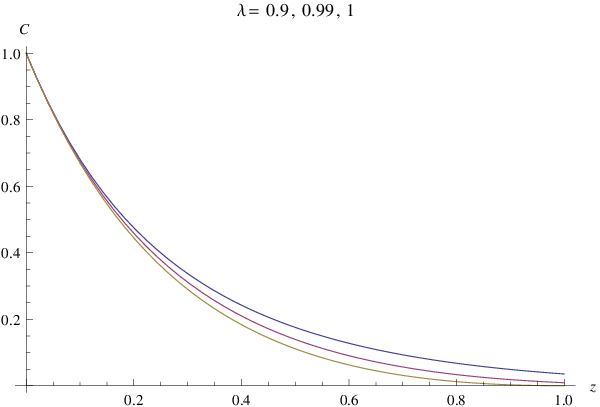
The first two curves are obtained from the Padé approximants of the small time expansion in . The last curve is the function .
The curves show that the Padé approximants give an accurate description of the function at time smaller that 1, and that the limit is achieved smoothly.
II.1 Aging
The previous analysis can be generalized to the aging dynamics. We specialize to the case of the generalized spherical -spin model where the temperature appears explicitly into the equation. The structure of the equation in the aging alpha regime is similar to the equilibrium case and one has [19]
| (15) | |||
Here generalizes the memory kernel of the equilibrium case.
The quantity is the so called fluctuation-dissipation ratio, fixed by the condition that the function
| (16) | |||
has a double root in .
It is well known that equation (15) is reparametrization invariant and admit scaling solutions of the form where the reparametrization function is left undetermined. The short time expansion of the equation predicts a behavior of the kind
| (17) |
where is determined by the condition [18]
| (18) |
As in the equilibrium case, for close to the function behaves as . We can suppose that becomes an analytic function of . Notice that if the function is such that for large , then one can equivalently write . We can then define the scaling function
| (19) |
and repeat verbatim the analysis of the equilibrium case. It turns out that the equation verified by coincide with the one found at the critical point. A fortiori, the same is true for the function .
III Fluctuations
In this section we would like exploit our analysis to investigate fluctuations in the alpha regime. In the last years, research has concentrated in the study of fluctuations of the time dependent correlation functions in terms of 4-point functions. As often in disordered systems one can define different kinds of correlation functions with a-priori different scaling properties. It has been recently proposed that it is useful to disentangle the fluctuations of correlations with respect to thermal noise for fixed initial condition from the fluctuations with respect to initial conditions [20].
Denoting by the thermal average for fixed initial condition (iso-configurational average) and by the average initial condition, we define [21, 20]
| (20) | |||
A theory for this kind of fluctuations in the beta regime has been proposed in [20], using a ”reparametrization invariant” formulation where time is eliminated in favour of the average correlation function. Within a gaussian fluctuation theory it is found that the singularity of doubles the one of .
The basic observation allowing to study now the functions in the regime is the fact that, as proposed in [22], the leading behavior of can be obtained as
| (21) |
Before exploiting this relation we would like to note that it appears naturally in the theory put forward in [20]. In that context that fluctuations can be described through a field theory where the correlation function, which plays the role of fundamental field, couples linearly to the temperature. Moreover, the dependence with respect to the initial configuration turns out to be parameterized by a random variation of the temperature. This has the consequence that the susceptibility is the square of the thermal one multiplied by the variance of the random temperature.
While these consideration strictly hold for the beta and early alpha regime, the time-temperature superposition principle shows how the correlation is very sensitive to any temperature change which can induce large changes in the relaxation time. This is a sort of “beta imprinting” indicating that large fluctuations of the correlation fluctuations in the alpha regime could be just consequence of fluctuations in the initial time of relaxation. In last instance this is a consequence of the emerging scale invariance of the MCT equation when the critical temperature is approached. We see here a link with the theory of fluctuations during aging dynamics below developed by Cugliandolo, Chamon and collaborators [23, 24, 25, 26] where fluctuations are ascribed to the large time emergence of reparametrization invariance
With all this in mind, we can write:
| (22) | |||
Using the relation with for and , one gets
| (23) | |||
The divergence as a function of which just depends on the power law behavior of the relaxation time, confirms the direct dynamical analysis of [22].
Notice that for a finite system the divergence should be cut-off by a function of the volume. It was found in [27] and [20] that the scaling variable describing the cross-over is . This predict an alpha relaxation scaling at where and a finite .
In [20] it was shown that if follows a bimodal distribution as it would be implied by a simple jump process, one should expect the dependence . Notice the form we find differ form this expectation.
We would like to remark that while the square root behavior of at small is only valid in the limit of small that we are considering, the linear behavior for is more general: it is a consequence of the initial power law relaxation of the correlation function , that hold whenever there is a discontinuous transition. As far as the small behavior for finite is concerned, the final exponential relaxation suggests a behavior .
IV Conclusions
The point where the discontinuous transition becomes continuous can be seen as a critical point for Mode Coupling Theory. As such universal properties emerge which do not depend of the details of the model [1]. In this note we have computed the scaling functions for the correlation function both at the MCT transition and in the aging regime, finding that they take the same universal form. We have also analyzed the behavior of fluctuations, finding general expressions of the four point functions as a function of the correlations.
Acknowledgments
We thank G. Szamel for discussions. SF acknowledges hospitality of the Physics Department of the “Sapienza” University of Rome. The European Research Council has provided financial support through European Research Council Grant 247328.
References
- [1] W. Götze, Complex dynamics of glass-forming liquids: A mode-coupling theory, vol. 143 (Oxford University Press, USA, 2009).
- [2] G. Parisi and T. Rizzo, arXiv:1205.3360 (2012).
- [3] F. Caltagirone, U. Ferrari, L. Leuzzi, G. Parisi, F. Ricci-Tersenghi, and T. Rizzo, Phys. Rev. Lett. 108, 085702 (2012a).
- [4] F. Caltagirone, G. Parisi, and T. Rizzo, Physical Review E 85, 051504 (2012b).
- [5] U. Ferrari, L. Leuzzi, G. Parisi, and T. Rizzo, Physical Review B 86, 014204 (2012).
- [6] F. Caltagirone, U. Ferrari, L. Leuzzi, G. Parisi, and T. Rizzo, Physical Review B 86, 064204 (2012c).
- [7] S. Franz, H. Jacquin, G. Parisi, P. Urbani, and F. Zamponi, PNAS Early Edition www.pnas.org/cgi/doi/10.1073/pnas.1216578109 (2012).
- [8] T. Rizzo, arXiv:1209.5578 (2012).
- [9] U. Bengtzelius, W. Gotze, and A. Sjolander, Journal of Physics C: Solid State Physics 17, 5915 (1984), URL http://stacks.iop.org/0022-3719/17/5915.
- [10] V. Krakoviack, Physical review letters 94, 65703 (2005).
- [11] V. Krakoviack, Physical Review E 75, 031503 (2007).
- [12] W. Madden and E. Glandt, Journal of statistical physics 51, 537 (1988).
- [13] J. Given and G. Stell, The Journal of chemical physics 97, 4573 (1992).
- [14] C. Cammarota and G. Biroli, Proceedings of the National Academy of Sciences 109, 8850 (2012).
- [15] W. Gotze and L. Sjogren, Journal of Physics: Condensed Matter 1, 4203 (1999).
- [16] A. Crisanti and H. Sommers, Zeitschrift für Physik B Condensed Matter 87, 341 (1992).
- [17] A. Crisanti, H. Horner, and H. Sommers, Zeitschrift für Physik B Condensed Matter 92, 257 (1993).
- [18] J. Bouchaud, L. Cugliandolo, J. Kurchan, and M. Mézard, Physica A: Statistical Mechanics and its Applications 226, 243 (1996).
- [19] L. F. Cugliandolo and J. Kurchan, Phys. Rev. Lett. 71, 173 (1993).
- [20] S. Franz, G. Parisi, F. Ricci-Tersenghi, and T. Rizzo, The European Physical Journal E: Soft Matter and Biological Physics 34, 1 (2011).
- [21] L. Berthier and R. Jack, Physical Review E 76, 041509 (2007).
- [22] L. Berthier, G. Biroli, J. Bouchaud, W. Kob, K. Miyazaki, and D. Reichman, The Journal of chemical physics 126, 184503 (2007).
- [23] C. Chamon, F. Corberi, and L. Cugliandolo, Journal of Statistical Mechanics: Theory and Experiment 2011, P08015 (2011).
- [24] C. Chamon and L. Cugliandolo, Journal of Statistical Mechanics: Theory and Experiment 2007, P07022 (2007).
- [25] C. Chamon, P. Charbonneau, L. Cugliandolo, D. Reichman, and M. Sellitto, The Journal of Chemical Physics 121, 10120 (2004).
- [26] H. Castillo, C. Chamon, L. Cugliandolo, and M. Kennett, Physical review letters 88, 237201 (2002).
- [27] T. Sarlat, A. Billoire, G. Biroli, and J. Bouchaud, Journal of Statistical Mechanics: Theory and Experiment 2009, P08014 (2009).