An Affine Index Polynomial Invariant of Virtual KnotsThanks: The author was partially supported by UIC
Abstract.
This paper describes a polynomial invariant of virtual knots that is defined in terms of an integer labeling of the virtual knot diagram. This labeling is seen to derive from an essentially unique structure of affine flat biquandle for flat virtual diagrams. The invariant is discussed in detail with many examples,including its relation to previous invariants of this type and we show how to construct Vassiliev invariants from the same data.
Key words and phrases:
virtual knot, virtual link, writhe, Vassiliev invariant, quandle.2000 Mathematics Subject Classification
57M271. Introduction
This paper generalizes invariants of virtual knots defined by Z. Cheng [2] and by A. Henrich [11] to a new polynomial invariant of virtual knots and links. The invariant discussed herein is also related to the generalized parity invariants of H. Dye [5]. In all these cases, an invariant is constructed in terms of weights, , associated to the crossings of an oriented virtual knot and the invariants take the form of a polynomial defined by the equation
where denotes the sign of the crossing in the oriented knot The weights for the authors mentioned above are derived from the combinatorics of chord intersections in Gauss diagrams for the knots. In Cheng’s case the polynomial utilizes parity and the weights are restricted to odd crossings (crossings corresonding to chords that intersect an odd number of other chords in the Gauss diagram). In Henrich’s case the weights utilized are absolute values of the Cheng weights. The invariants in this paper are quite distinct from the index polynomial invariants discussed in [15, 13, 14], while these invariants follow a similar pattern in the form of the polynomial. We call the polynomial invariant given in this paper the Affine Index Polynomial because in our approach the polynomial is a way of assembling a set of crossing weights that are derived from a very simple affine biquandle structure on the underlying flat diagram. This affine structure is explained in detail in the body of the paper.
In this paper, we give a definition of weights that exhibits them as differences related to an integer labeling of a flat virtual diagram associated with the knot diagram. This makes the system of weights very easy to compute and one can then develop the invariant on this basis. We call the resulting polynomial the Affine Index Polynomial for an oriented virtual knot The paper is organized as follows. In section 2 we review the definitions of virtual knot theory and flat virtual knot theory. In section 3 we give the definition of the Affine Index Polynomial and one example. In section 4 we prove the invariance of the polynomial. In section 5 we give a number of examples of computations of the invariant. We give examples where virtual knots with unit Jones polynomial are both shown to be non-classical and examples where this Index invariant cannot show that the knot is non-classical. We give examples where invertibility is detected and we give examples where the non-triviality of a flat virtual knot is detected. We also give examples of cobordant knots and links that can be assigned an invariant. In section 6 we show that the following formulas give Vasiliev invariants of order :
where runs over all the crossings of the knot , is the sign of the crossing, and is the index of the crossing. In section 8 we analyse linear affine flat biquandles and show that for a full biquandle structure, the integer labeling that we have used to define the invariant is essentially unique. It is a consequence of this analysis that there are other affine flat pre-biquandles (made explicit in this section) that can be used to make invariants of flat virtuals without the third Reidemeister move (virtual doodles). This will be the subject of a separate investigation.
Acknowledgement. It gives the author great pleasure to thank Lena Folwaczny for many conversations and to thank the Newton Institute for Mathematical Sciences in Cambridge, UK for its hospitality in the final stages of the preparation of this paper.
2. Recollection of Virtual Knot Theory
This section is a quick recollection of the definition of virtual knot theory. For more information the reader is referred to [17, 10, 19, 20, 21, 24]. The diagrammatic definition of virtual knot theory is that virtual knots and links are represented by diagrams that are like classical knot and link diagrams, except that there is added a new crossing called a virtual crossing. The virtual crossing is here indicated by a flat crossing (neither over nor under) that is encircled by a transparent circle. See Figure 1 and Figure 2. In these figures we indicate how the classical Reidemeister moves are generalized to include moves that involve the virtual crossings. The general principle is that the virtual crossing behaves as an artifact of the projection of the virtual knot diagram to the plane. The actual virtual knot or link is independent of any embedding in the plane, but is assigned cyclic order of edges at each non-virtual crossing. Thus an attempt to embed the virtual knot in the plane can lead to extra crossings just as the embedding of a non-planar graph can require extra crossings. The moves for the virtual crossings are designed to respect this point of view. One can think of the virtual moves as generated by the local moves shown in Figure 1 or one can say that they are generated by classical Reidemeister moves plus the detour move shown in Figure 2. The detour move allows an arc with a consecutive sequence of virtual crossings to be excised and replaced any other such arc with consecutive virtual crossings.


The reader should take note of Figure 3 where we illustrate two moves on virtual knots that are not allowed and that do not follow from the given sets of moves. That these moves are forbidden is crucial in the structure of the theory. Allowing the move we obtain welded knot theory a different variant that is closely related to the theory of welded braids of Rourke, Fenn and Rimiyani [9].
Just as non-planar graphs may be embedded in surfaces of some genus, virtual knots and links can be represented by embeddings without virtual crossings in thickened orientable surfaces. In fact, the theory of virtual knots and links is equivalent to the theory of embeddings of circles in thickened surfaces modulo diffeomorphisms of the surfaces and one-handle stabilization of the surfaces. See [20, 1, 4, 24] for more information about this point of view.
2.1. Flat Virtual Knots and Links.
Flat virtual knots and links are defined in exactly the same way as virtual knots and links except that the classical crossings are replaced by flat crossings indicated by transversely intersecting line segments and no information about over or under crossing. In the diagram of a flat virtual link one has flat classical crossings and the (also flat) virtual crossings. The moves are exactly the moves indicated in Figures 1, 2, 3 with all crossings replaced by flat crossings. This means that once again we have forbidden moves, and it is easy to see that the presence of the forbidden moves gives flat virtual knot theory much non-trivial structure. In our construction of the Affine Index Polynomial, we shall be first make an invariant labeling structure of flat virtual knots, and then use it to make the invariant for regular virtual knots.
3. The Polynomial Invariant
We define a polynomial invariant of of virtual knots by first describing how to calculate the polynomial. We then justify that this definition is invariant under virtual isotopy. Calculation begins with a flat oriented virtual knot diagram (the classical crossings in a flat diagram do not have choices made for over or under). An arc of a flat diagram is an edge of the -regualar graph that it represents. That is, an edge extends from one classical node to the next in orientation order. An arc may have many virtual crossings, but it begins at a classical node and ends at another classical node. We label each arc in the diagram with an integer so that an arc that meets a classical node and crosses to the left increases the label by one, while an arc that meets a classical node and crosses to the right decreases the label by one. See Figure 4 for an illustration of this rule. We will prove that such integer labelling can always be done for any virtual or classical link diagram. In a virtual diagram the labeling is unchanged at a virtual crossing, as indicated in Figure 4. One can start by choosing some arc to have an arbitrary integer label, and then proceed along the diagram labelling all the arcs via this crossing rule. We call such an integer labelling of a diagram a Cheng coloring of the diagram.
Remark. That any virtual knot diagram can receive a Cheng coloring is analogous to the fact that diagrams can be Fox-colored in for appropriate values of In the case of Fox colorings there is a corresponding algebra structure - the quandle. In the case of the Cheng coloring we are looking at an example of a flat affine biquandle. We will discuss this algebraic background to the invariant in section 8 of this paper.


Given a labeled flat diagram we define two numbers at each classical node : and as shown in Figure 1. If we have a labeled classical node with left incoming arc and right incoming arc then the right outgoing arc is labeled and the left outgoing arc is labeled as shown in Figure 4. We then define
and
Note that
in all cases.
Definition. Given a crossing in a diagram we let denote the sign of the crossing. The sign of the crossing is plus or minus one according to the convention shown in Figure 5. The writhe, of the diagram is the sum of the signs of all its crossings. For a virtual link diagram, labeled in the integers according to the scheme above, and a crossing in the diagram, define by the equation
where refers to the underlying flat diagram for . Thus is according as the sign of the crossing is plus or minus. We shall often indicate the weight of a crossing in a knot diagram by rather than
Let be a virtual knot diagram. Define the Affine Index Polynomial of by the equation
where the summation is over all classical crossings in the virtual knot diagram We shall prove that the Laurent polynomial is a highly non-trivial invariant of virtual knots.
In Figure 4 we show the computation of the weights for a given flat diagram and the computation of the polynomial for a virtual knot with this underlying diagram. The knot is an example of a virtual knot with unit Jones polynomial. The polynomial for this knot has the value
showing that this knot is not isotopic to a classical knot. We will examine this example and others in the body of the paper.
4. Invariance of
In order to show the invariance and well-definedness of we must first show the existence of labelings of flat virtual knot diagrams, as defined in section 1. We shall do this by showing that any virtual knot diagram that overlies a given flat diagram can be so labeled.
Proposition. Any flat virtual knot diagram has a Cheng coloring.
Proof. Let be a flat virtual knot diagram. Label the arcs of by the following formula:
where denotes a classical crossing in is the sign of the crossing and denotes the set of crossings first met as overcrossings on traversing, in the direction of its orientation, the diagram starting at the arc The reader can easily check that this function satisfies the formulas in Figure 4 and Figure 6, and hence can be computed for by finding the value for a single arc, and then using the information on the underlying flat diagram to obtain all the other values. The change of across a classical crossing does not depend upon the sign of the crossing, but only on whether one is crossing to the right or to the left. It is the fact that is a signed sum of overcrossing encounters that makes its change independent of local crossing signs. This completes the proof of the Propposition. //

Note also that if we follow the algorithm of the section 1, Figure 4, to compute a labeling, the resulting labeling will differ from the labeling, defined above, by a constant integer at every label. Since the polynomial is defined in terms of the differences at each classical crossing of it follows that the weights as described in section 1, are well-defined.
We can now prove a useful result about the weights. Let denote the diagram obtained by reversing the orientation of and let denote the diagram obtained by switching all the crossings of is called the reverse of and is called the mirror image of
Proposition. Let be a virtual knot diagram and the crossing weights as defined in section 1 and above. If is an arc of let denote the corresponding arc of , the result of reversing the orientation of
- (1)
Let denote the label function, defined above, that counts overcrossings with signs. Then
where denotes the writhe of the oriented diagram
- (2)
Let be a crossing of and let denote the corresponding crossing of , then
- (3)
Consequently, we have
Similarly, we have
Thus this invariant changes to when the orientation of the knot is reversed, and it changes global sign and to when the knot is replaced by its mirror image.
- (4)
If is a classical knot diagram, then for each crossing in , and
Proof. The equation follows immediately from the fact that crossing signs are not changed in reversal of orientation and that where denotes the set of crossings first met as undercrossings on traversing, in the direction of the orientation of Thus
since the sum equals the writhe of for any arc in From this fact and the definition of as a difference of labels it is easy to calculate that The corresponding equation follows immediately from the definition of the polynomial. In the case of the mirror image, the sign of each crossing changes, and weights change sign. The formula is a consequence of that. Finally, if is a classical knot diagram and is a crossing in then The proof of this follows from the structure illustrated in Figure 7. In that figure we remind the reader that the labeling of an arc adds one when the arc crossings another arc going to the right and subtracts one when the arc crosses another arc going to the left. We wish to prove that if we start by labeling a oriented arc at a crossing and then continue the labeling until we emerge at an outgoing arc from that crossing, then the outgoing arc will receive the same label as the ingoing arc. This will be true if and only if the number of right-going arcs crossed in the loop are equal to the number of left-going arcs. First of all one can consider the loop that is traced in this journey. In a classical knot every crossing in that loop will be traversed twice, one with one handedness, and once with the opposite handedness. Thus there is zero total contribution from the self-crossings of the loop. What remains are the contributions from arcs that cross through the loop from the rest of the diagram. It is an easy Jordan curve argument to see that the total contributions from such curves is also zero (their self-crossings are irrelevant). The reader who examines Figure 7 will be able to supply the remaining details that reduce the arguement to an application of the Jordan curve theorem. Since in a classical knot we now know that for each crossing it follows that This completes the proof. //

Remark. We will give examples where mirror images and reversals are distinguished by in the next section. The argument showing that for crossings in a classical knot diagram can be used to understand when is either zero or not zero in a classical crossing in a virtual diagram. We will point out relevant examples in the next section.
We will now prove the invariance of under virtual isotopy. The reader will recall that virtual isotopy consists in the classical Reidemeister moves plus virtual moves that are all generated by one generic detour move. The (unoriented) virtual isotopy moves are illustrated in Figure 1 and Figure 2. In Figure 8 and Figure 9 we show the relevant information for verifying that is an invariant of oriented virtual isotopy.
Theorem. Let be a virtual knot diagram. Then the polynomial is invariant under oriented virtual isotopy and is hence an invariant of virtual knots.
Proof. Note that the definition of makes it independent of the moves in Figure 1 involving virtual crossings. The labeling algorithm is independent of the purely virtual moves and consequently the polynomial is invariant under them. Thus we need only verify invariance under the standard oriented Reidemeister moves, shown as box in Figure 1. Note that the Cheng coloring is uniquely inherited under the Reidemeister moves, and thus we only have to check the local changes in the coloring in relation to given types of move. Since we wish to verify invariance under oriented Reidemeister moves, we use the well-known fact (see [16] page 81) that it is sufficient to verify invariance under type I moves, two orientations of type II moves and the single instance of the type III move where there is a non-cyclic triangle in the center of the pattern and all the crossings have the same type (say positive). In Figure 8 we give the relevant information for the moves of type I and II. For the type I move, we see that the weight equals This means that the contribution of a diagram with a type I move at a crossing is equal to Since this is subtracted by the writhe in the formula we see that the polynomial is invariant under move I. For move II there are two cases or orientation as shown in the Figure 8. In each case, the move is available when the crossings have opposite sign. The calculation shown in the figure proves that when the crossings have opposite sign, the weights of the crossings are identical. Thus the sum of these two crossing contributions cancels out in the polynomial both in the -terms and in the writhe term. Therefore the polynomial is invariant under the II move. Finally, we examine the III move via the information in Figure 9. Here we assume that all three crossings are positive. The labels are calculated from flat versions of the move. We see that the resulting weights are simply permuted and the signs of the crossings remain unchanged. Thus the polynomial is invariant under move III. This completes the proof of the theorem. //
Generalization from Knots to Links. We are now in a position to generalize the invariant to some cases of virtual links and even to some cases of classical links. It is possible that a link diagram can be Cheng colored according to our rules. for example, view Figure 15 to see a labelling of the classical Hopf link. Before analyzing this figure, consider the proof we have given for the invariance of the polynomial Cheng coloring is uniquely inherited under Reidemeister moves and the weights at the three crossings of the third Reidemeister move are permuted under the move. These properties are true for the polynomial that we would write for any Cheng-colored link. Thus we can conclude that if we are given pair where is a link diagram and is a Cheng-coloring of this diagram, then the polynomial , defined just as before, is an invariant of the pair where a Reidemeister move applied to produces where is the diagram obtained from by the move, and is the coloring obtained from by the move.


5. Examples and Cobordisms
In this section we will give a number of examples of computations of the Affine Index Polynomial.
- (1)
We begin with the example in In Figure 4. Note since the Affine Index Polynomial for this knot is it follows that is not equivalent to its mirror image. This knot is an example of a virtual knot with unit Jones polynomial. We refer the reader to examine [17, 21] for the details of this construction. One can produce non-trivial virtual knots with unit Jones polynomial by the specific method of virtualizing a set of crossings in a classical knot that would produce a classical unknot when switched. See Figure 10. In this figure we illustrate virtualization of a crossing consisting in retaining it as an over or under crossing, but reversing its orientation. This is accomplished by redrawing the crossing, first scribing a virtual crossing, then performing the crossing with an opposite orientation, then scribing another virtual crossing. The result is a crossing that is flanked by two virtual crossings such that smoothing the two virtuals gives the original diagram with a switched crossing. The figure also illustrates how the bracket polynomial of a virtualized crossing is the same as the bracket polynomial of the original diagram with a switched crossing. Given a non-trivial classical knot , one can choose a subset of crossings so that the unknot is obtained if they are all switched. If we virtualize this same set of crossings, we obtain a non-trivial [17, 21] virtual knot with unit Jones polynomial. We conjecture that no such is virtually isotopic to a classical knot. This conjecture has so far only been verified in examples. The Affine Index Polynomial promises to be a useful tool in investigating this conjecture.

Figure 10. Switch and Virtualize - (2)
Figure 11 Illustrates an infinite family of virtual knots with the same Affine Index Polynomial.

Figure 11. A Family of Virtual Knots with the Same Polynomial - (3)
Figure 12 gives another example of virtualization. The knot has unit Jones polynomial but a non-trivial Affine Index Polynomial, proving that is not classcial. Then in Figure 13 and Figure 14 we illustrate how the appearance of zeroes in the list of vertex weights for the polynomial can be used to produce labelled knots and links where the crossings with null weights have been smoothed. We will call the smoothing indicated in Figure 13 a basic labeled cobordism. Thus if a knot has crossings with null weights, then it is labeled cobordant to a link with only non-zero weights (or an empty set of weights). While not all links can be labeled, this form of cobordism does produce labeled links, and the Index Invariant can be extended to such links as indicated in Figure 15. Here we write down the most general labeling for the link, and then deduce a set of variable integer exponents for the polynomial invariant. We shall leave the details of this generalization to another paper.
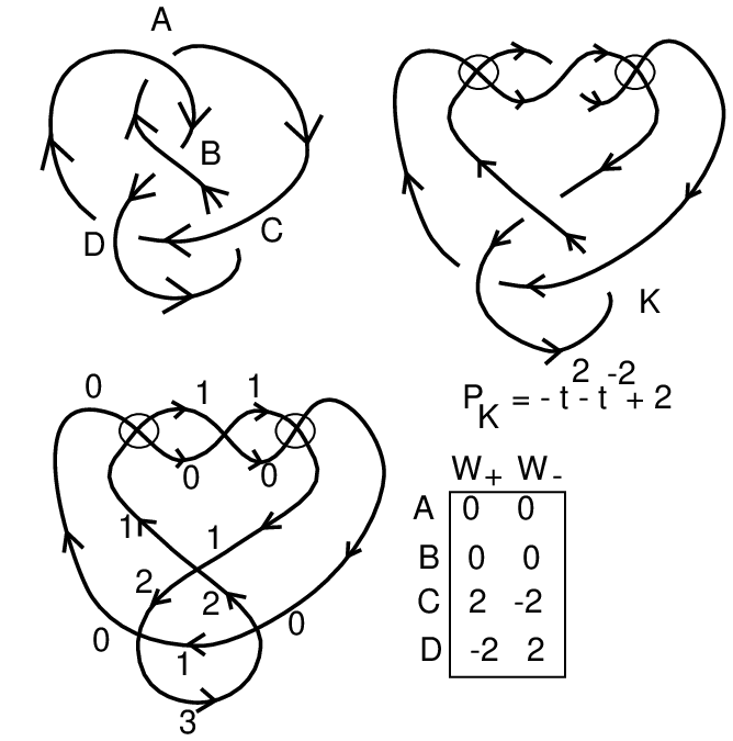
Figure 12. A Virtualization Example 
Figure 13. Basic Labeled Cobordism 
Figure 14. Labeled Cobordism of a Knot to a Link 
Figure 15. Invariant for the Hopf Link - (4)
In Figure 16 we give an example of a classical knot that can be transformed to an unknot by switching three crossings. This knot has unknotting number three. However when we take the corresponding virtualization, we find the the Index invariant is equal to zero. Thus the non-classicality of this virtualization is not detected by the Index invariant. This leads to a question that is worth investigating: Characterize those virtualizations that are detected by the Index invariant.

Figure 16. A Virtualization with Trivial Polynomial - (5)
In Figure 17 we give an example of a flat diagram such that the Index invariant is not zero for any choice of resolution for its crossings. This implies that the flat diagram is itself a non-trival virtual flat becuase it is not hard to see that if there were a flat isotopy that trivializes then it would be overlaid by an trivializing isotopy for some choice of crossings for the flat diagram. This example shows that one can sometimes use the Index invariant to detect non-trivial flat knots. In this last example we see from the Index invariant that all knots overlying this flat diagram are non-classical, non-invertible and inequivalent to their mirror images.

Figure 17. A Non-trivial and Non-invertible Flat Knot - (6)
In Figure 18 we illustrate a non-trivial knot with trivial Affine Index Polynomial. All the crossing weights are zero for this knot. Its non-triviality can be checked by computing its Jones polynomial. But the knot is not shown to be non-classical by the Arrow Polynomial [3], Arrow Polynomial Categorification [6, 7], or by the Sawollek Polynomial [18]. At this writing we do not know whether is non-classical but we conjecture that this is the case. It is not hard to make infinitely many examples of this kind (for example, by adding more twists to the given example) and so we are led to search for new invariants to detect non-classicality. A study of examples of this kind will be the subject of another paper.
Note added in proof. The example in Figure 18 has been shown to be non-classcial by M. V. Zenkina, using results in her paper [25] and it has been shown to be non-classcial by the Author and Slavik Jablan by using results in the paper by V. O. Manturov [22]. In the latter case, the relevant fact is Manturov’s Theorem that states the no classical knot has virtual representatives with the number of classical crossings less than its minimal crossing number as a classical knot.
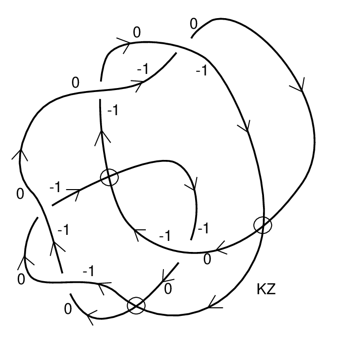
Figure 18. A Non-Trivial Knot With Zero Affine Index Polynomial
6. Vassiliev Invariants From the Affine Index Polynomial
The method of exponential substitution yields an infinite set of Vassiliev invariants for the Affine Index Polynomial. We show how to do this in the present section, and give specific formulas for these invariants in terms of the weights
Note that we have the following skein relation for the Affine Index Polynomial:
where denotes the crossing at which the switch occurs, and is a diagram with a positive crossing at and is the diagram with a negative crossing at that is obtained by changing just this one crossing. We leave the proof of this identity to the reader. Note that the comes from the writhe difference between the two diagrams.
We use the skein difference to extend the Affine Index Polynomial to an invariant of virtual -regular graph embeddings (See [17]) by defining
where denotes the original diagram with a graphical node at the site This formula then defines the graph invariant (by expansion into differences) for any virtual graph Let Then
where is the coefficient of in this power series. Note also, from the skein relation above, that
Since
for any integer , this implies that whenever has more than nodes. This means that whenever In turn, this means that is a Vassiliev invariant of order (A Vassiliev invariant is of order if it vanishes on graphs with more than nodes.)
To obtain formulas for these Vassiliev invariants, consider any Laurent polynomial
where the exponents are an increasing set of integers and the coefficients are also integers. Then
Thus the coefficient of in the exponential substution is
We have proved
Proposition. For the Index invariant, we have a finite type Vassiliev invariant of order given by the formula
where runs over all the crossings of the knot , is the sign of the crossing, and is the index of the crossing.
Remark.
- (1)
While we have used the polynomial to deduce these Vassiliev invariants, it is worth noting that they depend only on the signs and weights of the crossings.
- (2)
Note that since it follows that if is non-zero for any odd then is inequivalent to its reverse orientation
- (3)
It is easy to see that for any virtual knot since the sum of all the signed weghts is equal to the sum of all the across the underlying flat diagram. And this latter sum is zero because every edge label occurs with both a positive and a negative sign in the sum. However, (a Vassiliev invariant of order ) is often non-zero in many examples, showing that irreversibility can be detected at the level of a Vassiliev invariant of order two.
- (4)
A specific example that has this property is shown in Figure 17 with the specific knot with polynomial We then have the formula
Thus but proving (again) that is inequivalent to its reverse.
7. Flat Biquandles
We have seen that the Affine Index Polynomial is based upon a labeling of a flat virtual diagram by integers that follows the rule given in Figure 6. The form of this labeling, following the rules of this figure, is invariant under virtual isotopy in the sense that for each virtual move, there is a unique way to extend the labelling to the new diagram, changing it only locally at the site of the move. It is the purpose of this section to give the Affine Index Polynomial a context by discussing the algebraic structure behind this labeling. To this purpose we make the following definition.


Definition. A flat biquandle is an algebraic system with two binary operations denote and satisfying the following axioms.
- (1)
For each there is a unique such that and And for each there is a unique such that and
- (2)
For all
and
For all there exist unique elements such that
- (3)
For all
The motivation for this definition is supplied in Figure 19, Figure 20 and Figure 21. In Figure 19 we interpret the operations and in terms of labeling a flat diagram at a classical flat crossing. At a virtual crossing, there is no change in the labeling for arcs going through the virtual crossing. In this figure we show how the relation above corresponds to the flat first Reidemeister move and we show how the first part of relation above corresponds to the oriented flat second Reidemeister move. In Figure 20 we show how the second part of relation corresponds to the reverse oriented second Reidemeister move. Finally, in Figure 21 we show how relation above corresponds to invariance of labeling under the flat third Reidemeister move. This means that if a flat virtual diagram is consistently colored with the elements of a flat biquandle, then this coloring can be uniquely modified to produce colorings on diagrams that are equivalent to the given diagram under flat virtual equivalence. And also, we can define the flat biquandle for a virtual diagram by taking the free flat biquandle (in the sense of universal algebra) on labels for the arcs of the diagram (extending from classical crossing to classical crossing) modulo the relations introduced by the definition of operations in Figure 19. Flat biquandles have been studied in [12] and are called there semiquandles. We shall call an algebraic system that satisfies only and above a flat pre-biquandle. and for short we will use the term preflat. If is a preflat then it can be used to examine invariance under the first and second flat Reidemeister moves.
It is our purpose here to introduce flat biquandles in relation to the Affine Index Polynomial invariant for virtual knots and links. In particular, it is easy to see that the following structure on the integers is a flat biquandle:
This is exactly the underlying label rule for the Index polynomial. Thus we see that the underlying structure for this polynomial invariant is a very specific flat biquandle structure on the integers, that allows labeling of any flat virtual knot diagram. In this light of this, we wish to determine when a flat biquandle structure can be given by an affine formula of the following type:
Here we assume that the underlying set of the flat biquandle is a module over a commutative ring with elements of and specific elements of If these formulas define the structure of a flat biquandle on the set then we say that is an affine biquandle.
Theorem. Let be a module over a commutative ring with unit and no zero divisors. Let be any element of and let an invertible element of Then the following formulas define the general affine linear flat biquandle with coefficients in
and
When this flat biquandle is the root structure of the Index polynomial studied in the present paper. Note that we have chosen the notations to indicate that the operations in this flat biquandle are actually unary operations on the set
Proof. We begin with
and
We first look at the pair of equations
and
We then have
and
From the first equation we have
From this we conclude that we shall need that is invertible in and that
Putting this into the second equation, we have
Thus
Since this must be true for all , we require that the two coefficients vanish. Rewriting, we have
and
Now we turn to the second flat Reidemeister move.This corresponds to the equations
and
A calculation shows that
Thus we demand that
The analogous calculation with the other equation from the second move yields the further conditions
Using our assumption that the ring does not have zero-divisors, we conclude that either or Consider the case where It is easy to see that in this case the resulting operations are not invariant under the reversed orientation form of the second Reidemeister move. We leave this for the reader to verify. Therefore, we shall assume that and find that the equations reduce to
with
Now we apply the further condition of invariance under the reverse oriented Reidemeister two move. This is the requirement that there exist unique elements such that , , and Thus we have
Hence
Using these forms for and , we have as the equation
This is equivalent to the condition
Similarly, yields the condition
Thus we conclude that the following conditions will ensure invariance under the first and both of the second flat Reidemeister moves:
With and invertible, we have
so that
and
This is our final set of general equations for a possible linear affine flat biquandle. It then remains to check invariance under the flat third Reidemeister move. We checked this invariance by using a small computer program and found that it demands that Thus we are left with the equations
and
This completes the proof of the theorem.//

Remark. Our purpose in this section is put the index polynomial into the context of the flat biquandle. To this end, lets determine when one can use this flat affine biquandle of the above theorem to produce a weight system for a polynomial invariant. In Figure 22 we have illustrated a crossing with biquandle labels. We see from the figure that generalized weights at this crossing would be
and
In order to generalize our results that gave an invariant polynomial from the weight system, we need that
Lemma. In order to have with in a lableling by a general preflat, we need that
Proof. This follows immediately from the discussion above. //
Lemma. Let the preflat defined by the equations below be called the basic affine preflat:
This structure is a preflat by the argument in the last theorem (let ), and the weights defined as
and
satisfy the condition
Thus the basic affine preflat can be used to define invariants of flat oriented virtual diagrams up to the equivalence relation generated by the first and second flat Reidemeister moves.
Proof. We find
Thus we conclude that this preflat will yield a weight system for any value of This completes the proof of the Lemma. //
We leave it to the reader to check that for the more general preflat in the proof of the theorem, the restriction added by requiring that
gives exactly that and ) It follows that the basic affine preflat can be used to create pre-invariants of virtual knots where a pre-invariant is invariant under the first and second Reidemeister moves, but not invariant under the third flat Reidemeister move. The pre-invariant can be written formally as
where is a formal variable and denotes the weight of the crossing defined as above for a labeling of the knot by the preflat. This invariant also depends upon the choice of coloring of the knot diagram by elements of the preflat. To make an invariant that is dependent only on the diagram, one can form a further sum over all such colorings. There is more work to be done in this domain.
Remark. We can call flat virtual diagrams taken up to all oriented versions of the flat first and second Reidemeister moves virtual doodles following [8, 23]. In these papers by Fenn and Khovanov one considers flat link diagrams (not virtual) taken up to the equivalence relation generated by the first two Reidemeister moves. Study of virtual doodles will be undertaken in a separate paper.
Remark. In the theorem, we arrived at the affine biquandle given by the unary operations
and
It is easy to see that if a flat biquandle is defined by unary operations
and
then it suffices that these operations be inverses of one another with
for the structure to define a flat biquandle. We leave this verification to the reader.
Note that for this simple affine flat biquandle we have
Thus for the operations above, we have
We conclude that exactly when This shows that for a direct invariant there is no choice other then the very simple flat biquandle structure on which our Index polynomial is based.
References
- [1] J.S.Carter, S. Kamada and M. Saito, Stable equivalence of knots on surfaces and virtual knot cobordisms, in “Knots 2000 Korea, Vol. 1 (Yongpyong)”, JKTR 11, No. 3 (2002), 311–320.
- [2] Zhiyun Cheng, A polynomial invariant of virtual knots. arXiv:1202.3850
- [3] H. A. Dye and L. H. Kauffman , Virtual Crossing Number and the Arrow Polynomial, JKTR, Vol. 18, No. 10 (October 2009). Page: 1335-1357.
- [4] H. A. Dye and L. H. Kauffman, Minimal surface representations of virtual knots and links. Algebr. Geom. Topol. 5 (2005), 509–535.
- [5] H. A. Dye, Vassiliev Invariants from Parity Mappings. arXiv:1203.2939
- [6] H. A. Dye L. H. Kauffman and V. O. Manturov, (Chapeter 4) On two categorifications of the arrow polynomial for virtual knots. In M. Banagl and C. Vogel, editors, The Mathematics of Knots, Theory and Application, Vol. 1, Contributions in Mathematical and Computational Sciences, pp. 95-124, Heidelberg University, Springer-Verlag, 2011.
- [7] A. Kaestner and L. H. Kaufman. Parity, skein polynomials and categorification. JKTR, Vol. 21, No. 13 (2012), 1240011 - 124027. .http://front.math.ucdavis.edu/1110.4911
- [8] Fenn, R.; Taylor, P., Introducing doodles. Topology of low-dimensional manifolds (Proc. Second Sussex Conf., Chelwood Gate, 1977), pp. 37Ð43, Lecture Notes in Math., 722, Springer, Berlin, 1979.
- [9] R. Fenn, R. Rimanyi, C. Rourke, The braid permutation group, Topology 36 (1997), 123–135.
- [10] M. Goussarov, M.Polyak and O. Viro, Finite type invariants of classical and virtual knots, Topology 39 (2000), 1045–1068.
- [11] A. Henrich, A Sequence of Degree One Vassiliev Invariants for Virtual Knots. Journal of Knot Theory and its Ramifications 19, 4 (2010), pp. 461–487. arXiv:0803.0754
- [12] A. Henrich and S. Nelson, Semiquandles and flat virtual knots, Pacific Journal of Mathematics, Vol. 248 (2010), No. 1, 155–170.
- [13] , Y.H. Im, K. Lee, H. Son, An index polynomial for flat virtual knots, European J. Comb. 31, (2010), pp. 2130-2140.
- [14] Y.H. Im, K. Lee, H. Son, Index polynomial invariant of virtual links, JKTR Vol. 19, No. 5 (2010), pp. 709-725.
- [15] N. Kamada, Index polynomial invariants of twisted links, (to appear in JKTR).
- [16] L. H. Kauffman, “Knots and Physics”, Fourth Editiion (2012), World Sci. Pub. Co.
- [17] L. H. Kauffman, Virtual Knot Theory , European J. Comb. 20 (1999), 663–690.
- [18] L. H. Kauffman and D. E. Radford. Bioriented quantum algebras and a generalized Alexander polynomial for virtual links. in ”Diagrammatic Morphisms and Applications (San Fransico, CA 2000), 113-140. contemp. Math. 318, AMS, Providence, RI (2003)
- [19] L. H. Kauffman, A Survey of Virtual Knot Theory, Proceedings of Knots in Hellas ’98, World Sci. 2000, 143–202.
- [20] L. H. Kauffman, Detecting Virtual Knots, Atti. Sem. Mat. Fis. Univ. Modena Supplemento al Vol. IL (2001), 241–282.
- [21] L. H. Kauffman, Introduction to virtual knot theory, JKTR, Vol. 21, No. 13 (2012), 1240007 (37 pages), arXiv:1101.0665.
- [22] V. O. Manturov, A Functorial Map from Virtual Knots to Classical Knots and Generalisations of Parity, arXiv:1011.4640.
- [23] Khovanov, M., Doodle groups. Trans. Amer. Math. Soc. 349 (1997), no. 6, 2297Ð2315.
- [24] G. Kuperberg, What is a virtual link?, Algebraic and Geometric Topology 3 2003, 587–591.
- [25] M. V. Zenkina, The parity hierarchy and new invariants of knots in thickened surfaces, (to appear).