Floquet Majorana Fermions for Topological Qubits
Abstract
We introduce and develop an approach to realizing a topological phase transition and non-Abelian statistics with dynamically induced Floquet Majorana fermions (FMFs). When the periodic driving potential does not break fermion parity conservation, FMFs can encode quantum information. Quasi-energy analysis shows that a stable FMF zero mode and two other satellite modes exist in a wide parameter space with large quasi-energy gaps, which prevents transitions to other Floquet states under adiabatic driving. We also show that in the asymptotic limit FMFs preserve non-Abelian statistics and, thus, behave like their equilibrium counterparts.
pacs
74.78.Na, 03.67.Lx, 05.30.Pr, 74.40.GhIntroduction — Proposals of solid state [1, 2, 3, 4, 5, 6, 7] and cold atomic [8, 9, 10] systems hosting Majorana fermions (MFs) have been a recent focus of attention. These systems present novel prospects for quantum computation since a widely separated pair of MF bound states, that formally correspond to zero-energy states of an effective Bogoliubov-de Gennes (BdG) Hamiltonian, forms a nonlocal fermionic state that is immune to local sources of decoherence. Moreover, MFs obey non-Abelian statistics and thus have potential for topological quantum information processing. Among the key signatures of MFs are a zero-bias resonance in tunneling [11, 12], half-integer conductance quantization [13, 14], and a Josephson effect [15]. Some of these predictions have already received possible experimental support [16, 17, 18].
Topological states of matter can be induced dynamically by time-periodic driving, the so-called Floquet approach [19, 20, 21]. This brought to the agenda the new concept of Floquet Majorana fermion (FMFs) [10]. It turns out that even if the system is initially in the topologically trivial state, its Floquet version may exhibit topological properties. A realization of such states where they can be readily manipulated and precisely tuned in a wide parameter space is therefore highly desirable. The natural questions for FMF systems are: whether they are robust and tunable, whether they can encode quantum information, and whether they follow non-Abelian statistics as for their equilibrium counterparts. Our study aims to answer these questions.
We consider a generic platform to investigate non-Abelian statistics and potentially to realize topological quantum computation based on FMFs. The model is broadly applicable to both semiconductor-superconductors heterostructures with strong spin-orbit interaction and in-plane magnetic field [6, 7], and to cold atomic systems where superconducting order is controlled by Feshbach resonances while spin-orbit coupling and Zeeman field effects are induced by an optical Raman transition [10]. The latter realization is practically more promising since it allows a greater degree of control. Furthermore, atomic condensates can be isolated thus suppressing dissipation on long time scales.
We show, first, that if FMFs exist, they will exist at any instantaneous time. Therefore, FMFs can encode quantum information if the driving potential does not break fermion parity conservation. We study the quasi-energy spectrum of the problem analytically by using a rotating frame analysis in the limit that the frequency is large compared to the band width. We also perform exact numerical calculations which capture certain features of the spectrum beyond the rotating wave approximation (RWA). A broad range of parameters supporting FMFs is identified as a function of driving frequency and amplitude for three specific driving scenarios: periodic modulation of the chemical potential, or the Zeeman field. Finally, by using a two-time formalism [7, 8], we show that FMFs follow the same non-Abelian statistics as their stationary counterparts. This conclusion stems from the observation that a generalized Floquet Berry matrix does not affect the non-Abelian statistics of FMFs since large quasi-energy gap ensures no transitions to other Floquet quasi-energy states in the adiabatic movement.
Floquet Theorem for Majorana Fermion — Let us consider Floquet theory [24]. Suppose that the Hamiltonian has an explicit time dependence with period , where is the driving frequency. The solution of the Schrödinger equation can be described by a complete set of time-dependent state , where quasi-energies satisfy the equation and are Floquet states (hereafter ). The evolution operator has the following property
| (1) |
One can define an effective Hamiltonian through the relation [20, 21]
| (2) |
with . We treat as just a parameter. The effective Floquet Hamiltonian is defined at each instantaneous time, and the topological properties of each of these Hamiltonians is the same [20, 21].
If the system is described by a BdG Hamiltonian, the quasi-particle excitation spectrum will possess a particle-hole symmetry even if the time-dependent potential is added [20]. For any quasi-energy state , the relation is guaranteed. So, the zero quasi-energy state reveals the existence of a Floquet MF [10]. The full wavefunction for can be written as , with . Since quasi-energy is only defined in a interval of (e.g. from to ), another type of Floquet MF exists at with [10]. From the argument above, we can show that if the zero quasi-energy state exists, a zero energy Floquet MF mode exists at any instantaneous time . The MF operator evolves in time periodically ; in general, it is different at different instantaneous times, .
Quasi-Energy Spectrum and Floquet Majorana Fermion — To demonstrate the existence of FMFs consider a one dimensional wire with Rashba spin-orbit interaction , Zeeman splitting , and proximity-induced superconducting term . The system can be described by a tight-binding Hamiltonian [6, 7, 10]:
| (3) | |||||
Here, and denote fermion site and spin indices while are corresponding operators, is the hopping term along the chain which yields a band width , and is the chemical potential of the lattice model which is set to the particle-hole symmetric point [25]. Note that Hamiltonian Eq. (3) is equally generic for a system of cold atoms [10].
To add time dependence, it is natural to consider modulating one of the parameters in : the chemical potential, the spin-orbit coupling [28], or the Zeeman field. We first consider periodic modulation of the chemical potential; the Hamiltonian is with
| (4) |
where . To calculate the quasi-energy, one can choose a basis in the rotating frame [1]
| (5) |
where is the basis of the unperturbed system, and labels the photon sector of the Floquet basis. The quasi-energy can be obtained by diagonalizing the Floquet operator in this basis. The orthonormality condition of the Floquet states is only defined in an extended Hilbert space [2], so the inner product must include an extra time integral over a full period: . The matrix elements read
| (6) | |||||
Since different photon sectors are separated by an energy gap of order , in the limit , the admixture of photon sectors can be neglected; this is in essence the rotating wave approximation. Then, we can consider only the zero photon sector and obtain an effective Floquet Hamiltonian by computing the matrix element. The key point to notice is that only the superconducting term in (3) fails to commute with the chemical potential operator . Evaluation of Eq. (6) within the RWA yields an effective Floquet Hamiltonian with exactly the same form as with the pairing coupling effectively renormalized to
| (7) |
( is the zero order Bessel function of the first kind.)
We conclude from Eq. (7) that in Floquet systems one may induce a topological phase transition dynamically. Indeed, recall that the regime for a topological superconducting phase of , which supports MFs, requires the condition [6, 7, 25]. Even if initially this condition is not satisfied so that the system is in the topologically trivial state, the renormalization may make a topological phase possible since . Thus, periodic modulation of the chemical potential provides a way to tune the topological phase and so realize MFs by varying the parameter . The rescaling Eq. (7) holds only, of course, to the extent that off-diagonal couplings can be neglected; we address the generic case numerically below and show that more dramatic changes in behavior are entirely possible.
For periodic modulation of the Zeeman field, a similar analysis can be carried out by adding to . Since only the Rashba term in Eq. (3) does not commute with the Zeeman term, the spin-orbit parameter is modified in the effective Floquet Hamiltonian: . Thus, periodic Zeeman modulation cannot induce a topological phase transition if one keeps only the zero photon sector. However, numerical investigation beyond the RWA [keeping all off-diagonal blocks of the effective Floquet Hamiltonian ] reveals that FMFs do, in fact, appear, and so we now turn to our numerical results.

For numerical convenience we consider square-wave driving of the chemical potential or Zeeman field: for , and for (with ), and similarly for . The evolution operator for the full period reads then , and the quasi-energy spectrum is obtained numerically using Eq. (1). In all cases here, the parameters at any instantaneous time correspond in the static system to the topologically trivial phase.
The results for periodically modulated chemical potential are shown in Fig. 1. Clearly, one obtains stable Floquet Majorana zero modes (left panels) for a large range of parameters, as well as modes (upper right panel) [32]. Note that the parameters used in Fig. 1 are very far from those for which the RWA result Eq. (7) yields a FMF: here at all times, so no renormalized can yield a non-trivial phase. Nevertheless, FMF appear once surpasses a threshold . The figure shows that the threshold for an FMF can be very small compared to that for an FMF, and also that the quasi-energy gap can be tuned by varying . The splitting of a mode due to finite size effects is plotted in the right lower panel; it shows the expected decay of the level splitting as the number of sites, and hence the separation between the two FMF, increases.
The quasi-energy spectrum with periodic Zeeman splitting is shown in Fig. 2. It also reveals FMFs. We stress once again that to obtain FMF in this case, the RWA is not enough and off-diagonal blocks of the Floquet Hamiltonian are crucial.

Floquet Topological Qubit and Non-Abelian Statistics — A natural question is whether FMFs can form topological qubits, as their static counterparts do. FMF can certainly encode quantum information: an FMF exists at all instantaneous times, and neither chemical potential driving nor Zeeman driving changes the total fermion parity. Then, a more difficult question is whether FMFs obey non-Abelian statistics. We will provide an argument for a 2D system, which can then be generalized to a 1D network following the argument for static MF [29].
Suppose that FMFs are moved (which can be achieved by tuning the driving potential on and off, or changing the driving amplitude,) along a path with the Schrödinger equation . The position of the FMF is assumed to vary on a very slow time scale compared to the fast periodic driving. Then, it is convenient to separate the fast and slow time scales, and apply the two-time formalism of Floquet theory [7, 8]: , where indicates the fast time and denotes the slow time. Then the Schrödinger equation becomes
| (8) |
When we consider the dynamics on the slow time scale, the fast time can be considered as a parameter. It was pointed out by Breuer and Holthaus [7] (also see a recent discussion [30]) that a Floquet system follows a generalized adiabatic theorem. Define the instantaneous (for ) quasi-energy eigenstates using the Floquet operator
| (9) |
Suppose the system is initially in a Floquet state . Standard procedures in quantum mechanics can be applied to Floquet states as long as the extended inner product mentioned above, , is used. Second order perturbation theory then yields [7, 30]
| (10) |
where is the dynamical phase, and is the generalized Berry phase. Therefore, to avoid transitions to other quasi-energy states, the change in time scale must be slow and the quasi-energy gap should be large: . We assume this condition is satisfied so that the system will stay in its initial Floquet state.
The Floquet Majorana excitations can be described by a Bogoliubov quasi-particle operator,
| (11) |
where () creates (annihilates) a fermion at r, and for a MF. A gauge transformation which changes the superconducting order parameter phase by [3] is allowed by using the extended space of the Floquet system [32]. This causes a minus sign on both and , changing the sign of the FMF operator as well. Due to such multivaluedness, a branch cut is necessary to define the phase of the wave function. So, the exchange of two FMFs and can induce a transformation: and (since one of the FMF, say , must pass through the branch cut). For a 1D network, the exchange of two FMFs (through a T-junction, for instance) flips the sign of the superconducting pairing term, which results in exactly the same transformation as in the 2D case [29].
Given two FMFs and , one can form a non-local regular fermion . Let be the Floquet BCS state which is annihilated by any Floquet quasi-energy operators. and form a two-fold degenerate space. The exchange of two MFs results in and . The phase difference after the transformation signifies non-Abelian statistics [33, 34].
The exchange of two MF can also induce an extra unitary evolution involving a non-Abelian Berry matrix [9]. The form of the matrix can be generalized to a Floquet system [32] by replacing with ; the unitary evolution then reads
| (12) |
where denotes path-ordering and is the generalized non-Abelian Berry matrix [32]. We want to test whether causes any extra phase difference that breaks the non-Abelian statistics of FMFs. First, the non-diagonal matrix elements of are zero since fermion parity is conserved (as emphasized above this is true for all driving scenarios). Second, we follow a procedure similar to that for a stationary MF [33, 34] where the odd parity element is written as the sum of the even parity element and an extra term . It is just this term that might affect the the phase difference and so the non-Abelian statistics. By using Eq. (11) and the MF condition one finds
| (13) |
This term is exponentially small since it contains an overlap of wave functions for spatially separated MFs; furthermore, it actually vanishes in the adiabatic limit. We conclude that the non-Abelian Berry phase does not destroy the desired statistics of FMFs.
Summary — Periodic modulation of the chemical potential or the Zeeman field appears to be a promising way to produce FMFs, both of which can be realized in 1D cold atom condensates. We find that Floquet MFs are robust and can be generated in a wide parameter range. This system may have potential for topological quantum computation since FMFs obey the same non-Abelian statistics as their equilibrium counterparts.
D.E.L and A.L. acknowledge support from Michigan State University. The work at Duke was supported by US DOE, Division of Materials Sciences and Engineering, under Grant No. DE-SC0005237.
References
- [1] G. Moore and N. Read, Nuc. Phys. B 360, 362 (1991).
- [2] N. Read and D. Green, Phys. Rev. B 61, 10267 (2000).
- [3] L. Fu and C. L. Kane, Phys. Rev. Lett. 100, 096407 (2008).
- [4] J. D. Sau, R. M. Lutchyn, S. Tewari, and S. Das Sarma, Phys. Rev. Lett. 104, 040502 (2010).
- [5] J. Alicea, Phys. Rev. B 81, 125318 (2010).
- [6] R. M. Lutchyn, J. D. Sau, and S. Das Sarma, Phys. Rev. Lett. 105, 077001 (2010).
- [7] Y. Oreg, G. Refael, and F. von Oppen, Phys. Rev. Lett. 105, 177002 (2010).
- [8] M. Sato, Y. Takahashi, and S. Fujimoto, Phys. Rev. Lett. 103, 020401 (2009).
- [9] S.-L. Zhu, L.-B. Shao, Z. D. Wang, and L.-M. Duan, Phys. Rev. Lett. 106, 100404 (2011).
- [10] L. Jiang, T. Kitagawa, J. Alicea, A. R. Akhmerov, D. Pekker, G. Refael, J. I. Cirac, E. Demler, M. D. Lukin, and P. Zoller, Phys. Rev. Lett. 106, 220402 (2011).
- [11] K. T. Law, P. A. Lee, and T. K. Ng, Phys. Rev. Lett. 103, 237001 (2009).
- [12] J. D. Sau, S. Tewari, R. M. Lutchyn, T. D. Stanescu, and S. Das Sarma, Phys. Rev. B 82, 214509 (2010).
- [13] M. Wimmer, A. R. Akhmerov, J. P. Dahlhaus and C. W. J. Beenakker, New J. Phys. 13, 053016 (2011).
- [14] D. E. Liu and H. U. Baranger, Phys. Rev. B 84, 201308 (2011).
- [15] A. Y. Kitaev, Phys. Usp. 44, 131 (2001).
- [16] V. Mourik, K. Zuo, S. M. Frolov, S. R. Plissard, E. P. A. M. Bakkers, and L. P. Kouwenhoven, Science 336, 1003 (2012).
- [17] J. R. Williams, A. J. Bestwick, P. Gallagher, S. S. Hong, Y. Cui, A. S. Bleich, J. G. Analytis, I. R. Fisher, D. Goldhaber-Gordon, Phys. Rev. Lett. 109, 056803 (2012).
- [18] L. P. Rokhinson, X. Liu, and J. K. Furdyna, arXiv:1204.4212 (2012).
- [19] J.-i. Inoue and A. Tanaka, Phys. Rev. Lett. 105, 017401 (2010).
- [20] T. Kitagawa, E. Berg, M. Rudner, and E. Demler, Phys. Rev. B 82, 235114 (2010).
- [21] N. H. Lindner, G. Refael, and V. Galitski, Nat. Phys. 7, 490 (2011).
- [22] H. Breuer and M. Holthaus, Phys. Lett. A 140, 507 (1989).
- [23] S. C. Althorpea, D. J. Kouria, D. K. Hoffmanb, and N. Moiseyev, Chemical Physics 217, 289 (1997).
- [24] J. H. Shirley, Phys. Rev. 138, B979 (1965).
- [25] The chemical potential in Ref. [6, 7] is .
- [26] A. Eckardt, C. Weiss, and M. Holthaus, Phys. Rev. Lett. 95, 260404 (2005).
- [27] H. Sambe, Phys. Rev. A 7, 2203 (1973).
- [28] A. A. Reynoso and D. Frustaglia, arXiv:1208.2742v2 (2012).
- [29] J. Alicea, Y. Oreg, G. Refael, F. von Oppen, andM. P. A. Fisher, Nat. Phys. 7, 412 (2011).
- [30] T. Kitagawa, T. Oka, A. Brataas, L. Fu, and E. Demler, Phys. Rev. B 84, 235108 (2011).
- [31] D. A. Ivanov, Phys. Rev. Lett. 86, 268 (2001).
- [32] See supplementary materials for further details.
- [33] M. Stone and S.-B. Chung, Phys. Rev. B 73, 014505 (2006).
- [34] M. Cheng, V. Galitski, and S. Das Sarma, Phys. Rev. B 84, 104529 (2011).
- [35] F. Wilczek and A. Zee, Phys. Rev. Lett. 52, 2111 (1984).
I Supplementary Information
In this supplementary information we (i) provide more details about the rotating frame analysis (specifically, the derivation of Eq. (7) in the main text), (ii) provide more data on the quasi-energy spectrum, (iii) discuss gauge invariance in the extended space of Floquet system, and (iv) develop a generalization of the non-Abelian Berry matrix to Floquet system.
I.1 Derivation of Eq. (7) in the main text
We want to calculate matrix elements of the effective Floquet Hamiltonian in a basis of the rotating frame [1]. The starting point is Eq. (6) in the main text:
| (S14) | |||||
where is shown in Eq. (3) in the main text. We note that the operator fails to commute only with the superconducting term
| (S15) |
Therefore, we have
| (S16) | |||||
where is an anti-Hermitian operator
| (S17) |
Since different photon sectors (labeled by ) are separated by the energy , then in the limit ( is the band-width), we need consider only the zero photon sector, . This is the rotating wave approximation (RWA). Then, the effective Floquet Hamiltonian becomes
| (S18) |
Here, denotes zero order Bessel Function of the first type. The effective Floquet Hamiltonian within RWA has exactly the same form as in Eq. (3) in the main text except that the pairing coupling is renormalized to . Note that the integral of the second term, , is zero for . As we emphasized in the text, non-diagonal terms, , proportional to , may be important. We have given one example for the case of Zeeman field modulation.
I.2 More data for Quasi-energy spectrum
In the main text we showed a few representative examples of the quasi-energy spectrum as a function of driving period or amplitude. In this section we elaborate on this analysis and uncover a rather complicated structure of the quasi-energy states. This spectrum was found by numerical diagonalization keeping all the non-diagonal terms in the effective Floquet Hamiltonian.

Fig.S3 shows the quasi-energy spectrum as a function of driving period for square-wave chemical potential driving. As the driving amplitude increases from to , the Floquet MF in the region appears gradually, and the quasi-energy gap becomes larger for the FMF in the region . However, as the driving amplitude further increases, the quasi-energy gap becomes smaller (from to ) for FMFs in the region . The FMFs are even be killed for .

Fig. S4 shows the the quasi-energy spectrum near with periodic chemical potential as a function of driving period . Clearly, one can see the FMF mode appears in large region of parameter space. The quasi-energy spectrum near with periodic Zeeman splitting is shown in Fig. S5, which also reveals FMFs.

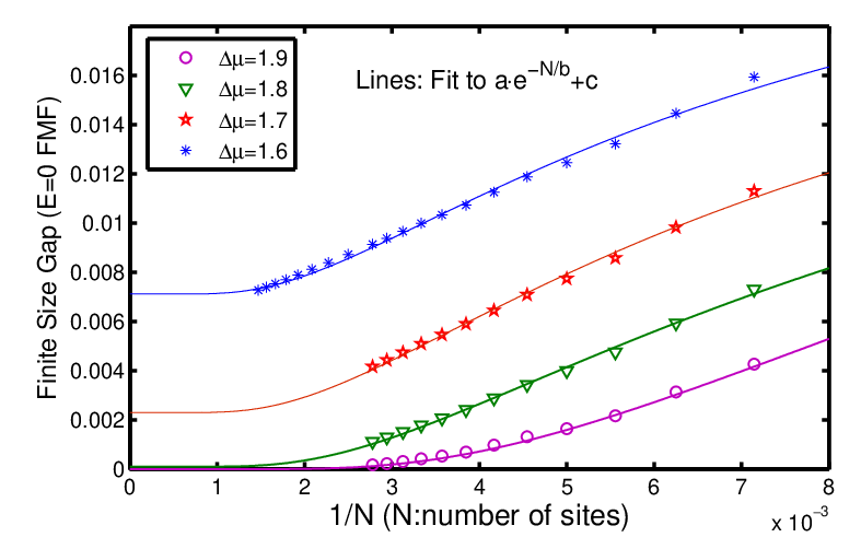
Fig. S6 shows finite size splitting, which indicates the coupling between two FMFs at wire ends, as a function of for the mode. is the number of sites in the chain. The splitting of two FMFs should decay exponentially as the length of the wire increase: , where the length of the wire with lattice spacing , and is the superconducting coherent length. We fit the data using the function form . As , the finite size splitting goes to zero for , and goes to finite values for , which shows the threshold for the FMF is larger than and smaller than .
One important quantity in Floquet theory is the mean energy [4] corresponding to the average expectation value of Hamiltonian over a full period: . Numerical data shown indicate that the partial derivative part of this expression vanishes for MF zero modes (except near the transition point), so and . Once weak heating effects are considered, one expects that the driven system tends to occupy the Floquet state with the lowest mean energy [5, 6]. Therefore, we focus on the FMF, that have the lowest mean energy.
I.3 gauge invariance in the extended space of Floquet system
For the system described by the BdG Hamiltonian, there is a gauge invariance [3]: if the global phase of the superconducting order parameter is shifted by , i.e. , it is equivalent to rotating electron creation and annihilation operator and .
Let us consider the instantaneous quasi-energy eigenstates (also shown in Eq. (9) in the main text)
| (S19) |
The quasi-energy state of the Floquet system is defined in a extended Hilbert space [2], therefore, one can expand the operator and state as the sum of different photon-sector [2]
| (S20) | |||||
| (S21) |
Then, the Floquet Hamiltonian of the extended Hilbert space can be written as
| (S22) |
It is easy to check that the invariance exists for all the matrix elements: . Therefore, the gauge invariance also exists for the Floquet system defined in the extended Hilbert space.
The Floquet MF excitations shown in Eq.(10) in the main text can also be written as
| (S23) |
where
| (S24) |
When the over all phase of the superconducting order parameter change , the Floquet MF excitation change sign: and thus .
I.4 Non-Abelian Berry Matrix for Floquet System
As shown in Eq.(8) in the main text, the adiabatic evolution of the Floquet system can be described by a two-time Schrödinger equation [7, 8] (also see Eq.(8) in the main text)
| (S25) |
Here, we will show if the quasi-energy degeneracy occurs in Floquet system, the adiabatic evolution of the Floquet system can be described by a generalized non-Abelian Berry matrix, as in the static counterpart [9].
Consider an instantaneous quasi-energy equation for a -fold degenerate Floquet states
| (S26) |
where . If the quasi-energy difference is large between this subspace and other states, the transitions to the states outside the -fold subspace can be neglected within the adiabatic approximation. For any time , the wave function of the system can be decomposed into a linear combination of the Floquet quasi-energy state
| (S27) |
Feed Eq. (S27) into Eq. (S25), one can obtain
| (S28) |
Projecting the equation to the state and carrying out the integral , one finds
| (S29) |
where
| (S30) |
corresponds to elements of the -by- matrix . Then, it is easy to check if the system is initially in the Floquet state , the time () evolution of such state can be written as
| (S31) |
where
| (S32) |
and denotes the path-ordering. This is the evolution operator given in Eq.(12) of the main text.
References
- [1] A. Eckardt, C. Weiss, and M. Holthaus, Phys. Rev. Lett. 95, 260404 (2005).
- [2] H. Sambe, Phys. Rev. A 7, 2203 (1973).
- [3] D. A. Ivanov, Phys. Rev. Lett. 86, 268 (2001).
- [4] A. G. Fainshtein, N. L. Manakov, and L. P. Rapoport, Journal of Physics B: Atomic and Molecular Physics, 11, 2561 (1978).
- [5] E. Arimondo, D. Ciampini, A. Eckardt, M. Holthaus, and O. Morsch, arXiv:1203.1259v2 (2012).
- [6] R. Ketzmerick and W. Wustmann, Phys. Rev. E 82, 021114 (2010).
- [7] H. Breuer and M. Holthaus, Phys. Lett. A 140, 507 (1989).
- [8] S. C. Althorpea, D. J. Kouria, D. K. Hoffmanb, and N. Moiseyev, Chemical Physics 217, 289 (1997).
- [9] F. Wilczek and A. Zee, Phys. Rev. Lett. 52, 2111 (1984).