1Introduction

FLAVOUR(267104)-ERC-25

BARI-TH/12-658

The Anatomy of Quark Flavour Observables
in 331 Models in the Flavour Precision Era
Andrzej J. Buras^a,b, Fulvia De Fazio^c, Jennifer Girrbach^a,b, Maria V. Carlucci^a
^aTUM Institute for Advanced Study, Lichtenbergstr. 2a, D-85747 Garching, Germany
^bPhysik Department, Technische Universität München, James-Franck-Straße,
D-85747 Garching, Germany
^cIstituto Nazionale di Fisica Nucleare, Sezione di Bari, Via Orabona 4, I-70126 Bari, Italy

Abstract

The coming flavour precision era will allow to uncover various patterns of flavour violation in different New Physics (NP) scenarios that are presently washed out by hadronic and experimental uncertainties. We illustrate this by performing the anatomy of flavour violation in the 331 models, based on the gauge group $SU(3)_{C}\times SU(3)_{L}\times U(1)_{X}$ that are among the simplest NP scenarios with new sources of flavour and CP violation. The latter originate dominantly through the flavour violating interactions of ordinary quarks and leptons with a new heavy $Z^{\prime}$ gauge boson. After discussing first these models in some generality, we present a detailed study of $\Delta F=2$ observables and of rare $K$ and $B$ meson decays in the specific “ $\beta=1/\sqrt{3}$ ” model (to be called $\overline{331}$ model) assuming significantly smaller uncertainties in CKM and hadronic parameters than presently available. The most prominent roles in our analysis play $\varepsilon_{K}$ , $\Delta M_{q}$ $(q=d,s)$ , the mixing induced CP asymmetries $S_{\psi K_{S}}$ and $S_{\psi\phi}$ , rare decays $B_{s,d}\to\mu^{+}\mu^{-}$ and in particular the CP-asymmetry $S_{\mu^{+}\mu^{-}}^{s}$ in $B_{s}\to\mu^{+}\mu^{-}$ . As the phenomenology of $Z^{\prime}$ contributions is governed only by $M_{Z^{\prime}}$ and four new parameters $\tilde{s}_{13}$ , $\tilde{s}_{23}$ , $\delta_{1}$ and $\delta_{2}$ , we identify a number of correlations between various observables that differ from those known from CMFV models. While, the $\Delta F=2$ observables allow still for four oases in the new parameter space, we demonstrate how the inclusion of $\Delta F=1$ observables can in the future identify the optimal oasis for this model. Favouring the inclusive value of $|V_{ub}|$ , for $1\,{\rm TeV}\leq M_{Z^{\prime}}\leq 3\,{\rm TeV}$ , the $\overline{331}$ model is in good agreement with the recent data for $B^{+}\to\tau^{+}\nu_{\tau}$ , it removes the $\varepsilon_{K}-S_{\psi K_{S}}$ tension present in the SM and the $\varepsilon_{K}-\Delta M_{s,d}$ tension present in CMFV models. Simultaneously, while differing from the SM, it is consistent with the present data on $\mathcal{B}(B_{s,d}\to\mu^{+}\mu^{-})$ and $S_{\psi\phi}$ . We identify the triple correlation $\mathcal{B}(B_{s}\to\mu^{+}\mu^{-})-S_{\psi\phi}-S_{\mu^{+}\mu^{-}}^{s}$ that constitutes an important test of this NP scenario.

1 Introduction

The LHCb experiment opened this year a new era of precision flavour physics [1]. This indirect route to shortest distance scales with the goal to discover new physics (NP) is also followed by ATLAS and CMS to be joined later in this decade in particular by SuperKEKB, SuperB in Rome and dedicated Kaon experiments NA62 at CERN, KOTO at J-Parc and ORKA at Fermilab.

While, as discussed below and reviewed in [2], there are several anomalies in the present data, none of them are conclusive and we should be prepared that NP effects in flavour observables will be present at most at the $50\%$ level of the Standard Model (SM) predictions and not an order of magnitude as initially expected and hoped for. In order to identify NP appearing at this level through flavour violating processes, it will be crucial to have both precise experiments and precise theory.

Indeed in indirect searches for NP through particle-antiparticle mixings in $K$ , $B_{s,d}$ and $D$ meson systems and rare decays of $K$ , $B_{s,d}$ and $D$ mesons it is crucial to know the background to NP: the predictions for various flavour observables within SM. If these predictions suffer from large uncertainties also the room left for NP is rather uncertain and if a given NP model contains many free parameters, the characteristic flavour violating features of this model cannot be transparently seen. They are simply often washed out by hadronic and parametric uncertainties even in the presence of accurate data. Most prominent examples of this type are the mass differences $\Delta M_{d,s}$ and the parameter $\varepsilon_{K}$ .

While the sophisticated model independent analyses of NP by professionals like UTfitters [3], CKMfitters [4], other bayesian [5] and frequentist analyses [6] and analyses using sophisticated Markov-chain Monte Carlos, in particular improved versions of the classical Metropolis algorithm [7, 8, 9, 10] should be appreciated, it is evident from the plots presented in these papers that several correlations between various observables are not clearly visible when all present hadronic and parametric uncertainties are taken into account.

In our view a complementary and a useful route to the identification of NP is a simplified approach in which one investigates how a given NP model would face the future more precise data with more precise hadronic and parametric input ¹¹ 1 The recent lattice results reviewed in [11, 12] and future experimental prospects [1, 13] assure us that the flavour precision era is just ahead of us.. In this manner some of the characteristic features of the particular NP model are not washed out and one discovers patterns of flavour violations, in particular correlations between different observables, that could distinguish between different NP models. While this approach has been already partially followed in the papers reviewed in [2], one recent study in this spirit of a concrete model shows that such studies could give interesting results.

Indeed, by proceeding in this manner and analysing the dependence of the allowed size of NP contributions in models with $U(2)^{3}$ flavour symmetry on the value of $|V_{ub}|$ , it was possible to identify the correlation $S_{\psi K_{S}}-S_{\psi\phi}-|V_{ub}|$ [14] characteristic for this class of models. This correlation was washed out in a much more sophisticated earlier analysis in [7] and could not be identified by these authors. Other similar examples in the literature could be given here.

While the more sophisticated analyses listed above are clearly legimitate and possibly could appear as the only way to analyze NP models at present, the example in [14] shows that it is also useful to work in a different spirit, even if it is a bit futuristic, and investigate how the pattern of flavour violation becomes visible when the uncertainties in CKM parameters and hadronic uncertainies are reduced. Such studies are not entirely new and can be found occasionally in various proposals, like the one in [13], but here we will illustrate them in a concrete model stressing the role of correlations between various observables that become visible in this approach. Our strategy is explained in concrete terms in Section 8.

One of the important questions in this context is whether the frameworks of constrained Minimal Flavour Violation (CMFV) [15] and the more general framework of MFV [16] will be capable of describing the future data. In models of this class, when flavour blind phases (FBPs) are absent or set to zero, stringent relations between various observables in $K$ , $B_{d}^{0}$ and $B_{s}^{0}$ systems are present [17]. Consequently the departures from Standard Model (SM) expectations in this class of models in these three meson systems are correlated with each other allowing very transparent tests of these simple NP scenarios. However, generally these relations can be strongly violated, implying often other correlations between observables characteristic for a given NP scenario. Such correlations being less sensitive to the model parameters can often allow a transparent distinction between various models proposed in the literature [18, 2]. In this manner the CMFV relations can be considered as standard candles of flavour physics [2].

Among the simplest extensions of the SM which go beyond the concept of MFV are the so-called 331 models based on the gauge group $SU(3)_{C}\times SU(3)_{L}\times U(1)_{X}$ (331) [19, 20]. Here the new sources of flavour and CP violation originate dominantly through the flavour violating interactions of ordinary quarks and leptons with a new heavy $Z^{\prime}$ gauge boson. Also one-loop contributions involving new charged gauge bosons and new heavy quarks with exotic electric charges can be relevant in certain processes.

The difference between the 331 models and CMFV models can be transparently seen in the formulation of FCNC processes in terms of master one-loop functions [17]. This formulation can be used here because the 331 models have the same operator structure as the SM and the CMFV models except that the real and universal master functions in the latter models become here complex quantities and the property of the universality of these functions is lost. Consequently the usual CMFV relations between $K$ , $B_{d}$ and $B_{s}$ systems can be significantly violated. Explicitly, the new functions in the 331 models, similarly to the case of the LHT model [21], will be denoted as follows ( $i=K,d,s$ ):

S_{i}\equiv|S_{i}|e^{i\theta_{S}^{i}},\quad X_{i}\equiv\left|X_{i}\right|e^{i\theta_{X}^{i}},\quad Y_{i}\equiv\left|Y_{i}\right|e^{i\theta_{Y}^{i}},\quad Z_{i}\equiv\left|Z_{i}\right|e^{i\theta_{Z}^{i}}\,,

(1)

Explicit expressions for these functions in specific 331 models will be given in the course of our presentation.

In 2007 two detailed analyses of flavour violation in the minimal 331 model to be defined below have been presented [22, 23]. During the last five years a number of changes both in the experiment and theory took place so that a new analysis of this model and other 331 models is required. In particular:

•

The $\varepsilon_{K}-S_{\psi K_{S}}$ tension in the SM has been identified [24, 25, 26, 27, 28, 29].
•

The branching ratio for $B^{+}\to\tau^{+}\nu_{\tau}$ has been found to be roughly by a factor of two larger than the SM prediction, even though the most recent data seem to be consistent with the SM (see Section 5).
•

The new lattice input appears to imply some tension between $\varepsilon_{K}$ and the mass differences $\Delta M_{s,d}$ within the CMFV models [2].
•

Most importantly the recent LHCb, ATLAS and CMS data imply SM-like values for $\mathcal{B}(B_{s}\to\mu^{+}\mu^{-})$ and for the mixing induced asymmetry $S_{\psi\phi}$ in the $B_{s}$ system, whereas in 2007 still large departures from SM predictions for both observables were possible.

The goal of the present paper is to make a fresh look at 331 models and to confront their flavour and CP violation structure with recent very improved data on $S_{\psi\phi}$ and rare decays $B_{s,d}\to\mu^{+}\mu^{-}$ from the LHCb, ATLAS and CMS taking into account the most recent lattice input that has a definite impact on various observables, in particular CMFV relations. Therefore in addition to $S_{\psi\phi}$ and $B_{s,d}\to\mu^{+}\mu^{-}$ we address simultaneously the $\varepsilon_{K}-S_{\psi K_{S}}$ tension still present in the SM, the mass differences $\Delta M_{s,d}$ , the rare decays $K^{+}\rightarrow\pi^{+}\nu\bar{\nu}$ and $K_{L}\rightarrow\pi^{0}\nu\bar{\nu}$ and the tree-level decay $B^{+}\to\tau^{+}\nu_{\tau}$ . We will also consider $K_{L}\to\mu^{+}\mu^{-}$ , $B\to X_{s,d}\nu\bar{\nu}$ and $B\to X_{s}\gamma$ , while leaving the analysis of $B\to X_{s}\ell^{+}\ell^{-}$ and $B\to K^{*}\ell^{+}\ell^{-}$ for the future.

We should announce already at this stage that in 2012 the minimal 331 model analyzed in [22, 23], the so-called “ $\beta=\sqrt{3}$ ”-model, does not imply any longer an interesting phenomenology of processes considered by us: new physics (NP) effects are simply very small. Therefore, we will dominantly discuss non-minimal 331 models with $\beta\not=\sqrt{3}$ . While a significant part of our presentation will apply to arbitrary $\beta$ , we will present a detailed phenomenology of flavour observables in a specific 331 model with $\beta=1/\sqrt{3}$ to be named $\overline{331}$ model in what follows. This model, while being rather economical, implies much more interesting phenomenology than the minimal model. In particular, while consistent with the present data, among rare decays, the largest deviations from SM expectations are found in $B_{s,d}\to\mu^{+}\mu^{-}$ branching ratios and the CP asymmetries $S_{\mu^{+}\mu^{-}}^{s,d}$ in $B_{s,d}\to\mu^{+}\mu^{-}$ , recently introduced in [30, 31].

Our paper is organized as follows. In Section 2 we recall in some details basic features of 331 models that are relevant for understanding of our analysis. In particular, we derive all Feynman rules for this class of models that we need for our phenomenology. In Section 3 we present the formulae for the effective Hamiltonians governing particle-antiparticle mixings $K^{0}-\bar{K}^{0}$ and $B_{d,s}-\bar{B}_{d,s}$ that in addition to the usual SM box diagrams receive tree-level contributions from $Z^{\prime}$ exchanges and new box diagram contributions. We also give a compendium of formulae relevant for numerical analysis of $\Delta F=2$ observables. In Section 4 the effective Hamiltonians for $s\to d\nu\bar{\nu}$ , $b\to q\nu\bar{\nu}$ , $b\to q\ell^{+}\ell^{-}$ ( $q=d,s$ ) and $b\to s\gamma$ transitions are given. In particular we present an improved QCD analysis of $Z^{\prime}$ contribution to $B\to X_{s}\gamma$ , demonstrating that it is negligibly small compared to the SM contribution. In Section 5 we calculate the most interesting rare decay branching ratios in the $K$ and $B$ meson systems, including those for the processes $K^{+}\rightarrow\pi^{+}\nu\bar{\nu}$ , $K_{L}\rightarrow\pi^{0}\nu\bar{\nu}$ , $B\to X_{s,d}\nu\bar{\nu}$ , $B_{s,d}\to\mu^{+}\mu^{-}$ , $B^{+}\to\tau^{+}\nu_{\tau}$ and $K_{L}\to\mu^{+}\mu^{-}$ . In Section 6 we recall the most important CMFV relations with the goal to find out how these relations are violated in the 331 models. In Section 7 we emphasize stringent relations between various observables in the 331 models that originate in the dominance of NP contributions by the tree-level $Z^{\prime}$ exchanges. In fact even without a detailed numerical analysis, it will be possible to deduce from these relations the pattern of deviations from the SM expectations predicted by the $\overline{331}$ model. In Section 8 we present first our strategy for numerical analysis and summarize the recent LHCb data and new lattice input. Subsequently, we demonstrate how already $\Delta F=2$ observables allow to identify four allowed oases in the new parameter space. We demonstrate how the inclusion of $\Delta F=1$ observables can in the future select the optimal oasis for this model. In this context the branching ratios $\mathcal{B}(B_{s,d}\to\mu^{+}\mu^{-})$ , the CP-asymmetry $S_{\mu^{+}\mu^{-}}^{s}$ in $B_{s}\to\mu^{+}\mu^{-}$ and $S_{\psi\phi}$ , when considered simultaneously, play the prominent roles. The correlations between these observables in the $\overline{331}$ model should allow to monitor how this model will face the data in the coming years. We also analyze how these correlations differ from the ones present in the CMFV models. The highlights of our analysis are listed in Section 9. There we also make a comparison of our findings with those known from other simple models. Few technicalities are collected in Appendices.

2 Flavour Structure of the 331 Models

2.1 Preliminaries

Among the many scenarios that have been proposed to extend the Standard Model (SM), one with rather appealing features is that based on the gauge group $SU(3)_{C}\times SU(3)_{L}\times U(1)_{X}$ , originally developed in [19, 20]. This group is spontaneously broken to the SM group $SU(2)_{L}\times U(1)_{X}$ , subsequently broken down to $U(1)_{Q}$ . Therefore, the 331 model has an extended Higgs sector [32], with the first symmetry breaking occurring at a scale much larger than the electroweak scale.

One of the nice features of this model is that the requirement of anomaly cancelation, together with that of asymptotic freedom of QCD, constrains the number of generations to be equal to the number of colours, thus providing an explanation for the existence of 3 generations, long sought for in the SM. Requirement of anomaly cancelation has also consequences on the transformation properties of fermions. In fact, as a first consequence of the extension of the SM gauge group $SU(2)_{L}$ to $SU(3)_{L}$ , one has that left-handed fermions transform as triplets (or antitriplets) under the action of $SU(3)_{L}$ . In order to have an anomaly-free theory, the number of triplets should be equal to the number of antitriplets. A possible choice is to assume that the three lepton generations transform as antitriplets, so that, taking into account the three colour possibilities for the quarks, the number of quark triplets should be equal to the number of antitriplets plus one. Hence two quark generations should transform as triplets, one as an antitriplet. The common choice of having the third generation with different transformation properties might be at the origin of the large mass of the top quark with respect to the other quarks. However, in contrast to the SM, where anomaly is canceled for each generation of fermions, in the 331 model the cancelation is fulfilled only when all the generations are considered.

As for the content of the (anti)triplets, the upper two components coincide with the known SM fermions. In the case of quarks, the third members of the generations correspond to new heavy quarks, while for leptons different choices are possible. The minimal version of the model makes the choice that no new leptons are introduced, so that the third component of the lepton antitriplet is chosen as the conjugate of the charged lepton (in practice, all the three possible helicity states for the SM leptons are contained). In this minimal version, among the three new heavy quarks two have charge $-\displaystyle{4\over 3}$ and one $\displaystyle{5\over 3}$ . Other variants are possible. In particular, in the lepton sector, another possibility could be that of having new heavy neutrinos as third components of the lepton antitriplets [33]. Indeed in the present analysis we choose a variant of this latter kind that has phenomenological implications that are more interesting than found in the minimal model.

The extension of the SM gauge group $SU(2)_{L}$ to $SU(3)_{L}$ also implies the existence of 5 new gauge bosons. These are a new neutral boson ( $Z^{\prime}$ ) plus other four that might be charged depending on the variant of the model that one chooses. We denote them generically as $V^{\pm Q_{V}}$ and $Y^{\pm Q_{Y}}$ . As we shall see when describing the model in details, the new bosons $V^{\pm Q_{V}}$ and $Y^{\pm Q_{Y}}$ couple two SM leptons, while this is not possible for SM quarks, which can only be coupled to new heavy quarks by means of these gauge bosons. Therefore the latter are assigned lepton number $L=\mp 2$ , but carry no lepton generation number so that the lepton generation number can be violated and indeed processes like $\mu\to e\gamma$ or $\mu\to 3e$ might proceed due to such new gauge boson mediation. Therefore, bounds on this model could come from the MEG experiment [34] the physics programme of which is devoted to the search for the lepton flavour violating process $\mu\to e\gamma$ . Detailed studies of the lepton sector of the model have been performed in [35, 36], in particular in [35] a mechanism to suppress large CP violation in this sector as well as large leptonic electric dipole moments was found.

The new neutral gauge boson $Z^{\prime}$ also introduces new features with respect to the SM as well as with respect to other NP scenarios that also contain a new neutral $Z^{\prime}$ , as for example grand unified theories (GUTs). In fact, in contrast to most of them, the $Z^{\prime}$ mass in some 331 models cannot be arbitrary, but is limited from above. ²² 2 Another similar case is for example represented by heterotic string models with supergravity mediated supersymmetry breaking [37] where also the $Z^{\prime}$ mass cannot be larger than around a TeV. This occurs because the $U(1)_{X}$ gauge coupling $g_{X}$ and the $SU(3)_{L}$ one $g$ are related by:

{g_{X}^{2}\over g^{2}}={6\sin^{2}\theta_{W}\over 1-(1+\beta^{2})\sin^{2}\theta_{W}}

(2)

where $\theta_{W}$ is Weinberg angle and $\beta$ is a parameter of the model (see next subsection) that defines its variants. Therefore, considering for example the minimal model with $\beta=\sqrt{3}$ , one should require $\sin^{2}\theta_{W}(M_{Z^{\prime}})<\displaystyle{1\over 4}$ . Since we know that $\sin^{2}\theta_{W}(M_{Z})\simeq 0.23$ , the evolution up to $M_{Z^{\prime}}$ constrains $M_{Z^{\prime}}$ below a few TeV [38]. On the other hand for $\beta=1/\sqrt{3}$ , as dominatly considered in our paper, this bound does not apply.

Also lower bounds on $M_{Z^{\prime}}$ were discussed in literature, stemming from study of $\mu$ decay within the model [38, 35, 39], from the analysis of $S$ , $T$ , $U$ parameters [33] and from comparison with experimental results from CDF Collaboration for possible $Z^{\prime}$ decays to $e^{+}\,e^{-}$ or $\mu^{+}\mu^{-}$ [40]. In principle those bounds are model dependent, since they depend also on the entries of the unitarity matrices that transform the quark gauge eigenstates into mass eigenstates. However, taking into account the results of the aforementioned analyses, we adopt as working range $1\,{\rm TeV}\leq M_{Z^{\prime}}\leq 3\,{\rm TeV}$ , which also shows that present experiments, mainly those at the LHC, have the possibility to test the model in the nearby future. Along the same lines, a possible mixing angle between the SM $Z$ and the new $Z^{\prime}$ has been considered, with the result that $\theta_{Z-Z^{\prime}}<{\cal O}(10^{-3})$ [40]. In what follows we will neglect this mixing.

The main novelty with respect to the SM related to the $Z^{\prime}$ is the existence of tree level flavour changing neutral currents (FCNC). However, these arise only in the quark sector, since the universality of the coupling of the $Z^{\prime}$ to leptons guarantees that no FCNC show up in this case. Furthermore, universality is also realized in the $Z^{\prime}$ couplings to right-handed quarks, so that the new FCNC are purely left-handed. The relevant couplings in this case are anyway small enough to make such tree level transition not larger than the corresponding loop induced SM contribution. Many processes induced by FCNC have been considered in the framework of the 331 model. Mixing of neutral mesons as well as a number of rare $K$ and $B_{d,s}$ decays have been considered in [39, 41]. Some of the results have been updated in [22], with particular attention to the neutral meson mixing and the study of possible new CP violating effects. The main result contained there is that the most sensitive quantity is the phase of $B_{s}$ mixing $\beta_{s}$ , as determined from $B_{s}\to J/\psi\phi$ . This is partly a consequence of the expectation that purely hadronic decays are potentially more sensitive to the $Z^{\prime}$ contributions since in addition to being flavour violating, the flavour conserving couplings of $Z^{\prime}$ to quarks is enhanced with respect to its coupling to leptons. We shall see this explicitly below. Finally, $b\to s\gamma$ was considered in [42] and reanalysed in [23]. Notice that this mode is loop-induced also in the 331 model.

As a final remark, we mention that the 331 model naturally possesses the Peccei-Quinn symmetry [43], solving the strong CP problem [44].

2.2 The Model

2.2.1 Gauge Bosons

In this section we provide a description of the 331 model in general terms and some of its variants parametrized by $\beta$ .

Leaving aside the case of $SU(3)_{C}$ , that presents no differences with respect to the SM, the generators of the gauge group are: $T^{a}=\displaystyle{\lambda^{a}\over 2}$ for $SU(3)_{L}$ ( $\lambda^{a}$ being the Gell-Mann matrices and $a=1,\dots 8$ ) plus $T^{9}$ which generates $U(1)_{X}$ . $T^{9}$ can be conveniently defined as $T^{9}=\displaystyle{\mathbb{1}\over\sqrt{6}}$ , the unit matrix being $3\times 3$ , when acting on triplets and just 1 when acting on singlets. With this definition, the generators satisfy the same relation as the eight generators of $SU(3)$ : $Tr[T^{a}T^{b}]=\displaystyle{\delta^{ab}\over 2}$ . In the case of antitriplets, transforming as $\bar{3}$ , the generators are $\bar{T}^{a}=-(T^{a})^{T}$ , $T$ meaning transpose.

The gauge bosons of the group $SU(3)_{L}$ are denoted as $W^{a}$ , $a=1,\dots 8$ and transform according to the adjoint representation of the group, while the gauge boson of $U(1)_{X}$ is denoted by $X$ . As a consequence, the covariant derivatives acting on the various fields read as follows:

•

triplet $\psi_{L}$ : $D_{\mu}\psi_{L}=\partial_{\mu}\psi_{L}-i\,g\,W^{a}_{\mu}T^{a}\,\psi_{L}-ig_{X}\,X\,X_{\mu}T^{9}\psi_{L}$ ;
•

antitriplet $\bar{\psi}_{L}$ : $D_{\mu}\bar{\psi}_{L}=\partial_{\mu}\bar{\psi}_{L}+i\,g\,W^{a}_{\mu}(T^{a})^{T}\,\bar{\psi}_{L}-ig_{X}\,X\,X_{\mu}T^{9}\bar{\psi}_{L}$ ;
•

singlet $\psi_{R}$ : $D_{\mu}\psi_{R}=\partial_{\mu}\psi_{R}-ig_{X}\,X\,X_{\mu}T^{9}\psi_{R}$ .

In the previous formulae, $g$ , $g_{X}$ denote coupling constants and $X$ is the new quantum number corresponding to $U(1)_{X}$ .

The matrix $W^{a}T^{a}$ can be rearranged as follows:

W_{\mu}=W^{a}_{\mu}T^{a}={1\over 2}\,\left(\begin{array}[]{ccc}W_{\mu}^{3}+{1\over\sqrt{3}}W_{\mu}^{8}&\sqrt{2}W_{\mu}^{+}&\sqrt{2}Y_{\mu}^{Q_{Y}}\\ \sqrt{2}W_{\mu}^{-}&-W_{\mu}^{3}+{1\over\sqrt{3}}W_{\mu}^{8}&\sqrt{2}V_{\mu}^{Q_{V}}\\ \sqrt{2}Y_{\mu}^{-Q_{Y}}&\sqrt{2}V_{\mu}^{-Q_{V}}&-{2\over\sqrt{3}}W_{\mu}^{8}\end{array}\right)

(3)

where the following definitions have been introduced:

$\displaystyle W_{\mu}^{\pm}$	$\displaystyle=$	$\displaystyle{1\over\sqrt{2}}(W_{\mu}^{1}\mp i\,W_{\mu}^{2}),$	(4)
$\displaystyle Y_{\mu}^{\pm Q_{Y}}$	$\displaystyle=$	$\displaystyle{1\over\sqrt{2}}(W_{\mu}^{4}\mp i\,W_{\mu}^{5}),$	(5)
$\displaystyle V_{\mu}^{\pm Q_{V}}$	$\displaystyle=$	$\displaystyle{1\over\sqrt{2}}(W_{\mu}^{6}\mp i\,W_{\mu}^{7}).$	(6)

$W^{3}$ and $W^{8}$ correspond to neutral gauge bosons; $W^{\pm}$ to the charged gauge bosons of the SM, while $V^{\pm Q_{V}}$ and $Y^{\pm Q_{Y}}$ might be charged or neutral. In order to assess this precisely, we have to define the electric charge matrix. In analogy with the SM, we introduce the following operator:

	$\displaystyle{\hat{Q}}_{W}$	$\displaystyle=$	$\displaystyle{\hat{T}}^{3}+{{\hat{Y}}\over 2}$		(7)
	$\displaystyle{{\hat{Y}}\over 2}$	$\displaystyle=$	$\displaystyle\beta{\hat{T}}^{8}+X\mathbb{1}\,\,.$		(8)

The constant $\beta$ that has been just introduced plays a key role in the model: according to its value various versions of the model have been proposed, which significantly differ from each other. In particular, only for some values of $\beta$ the gauge bosons turn out to have integer charges. In the case of the minimal 331 model, the choice $\beta=\sqrt{3}$ is adopted.

Even though we shall recall the features of the minimal model, we shall instead consider the variant with $\beta=\displaystyle{1\over\sqrt{3}}$ , which is phenomenologically more interesting than the $\beta=\sqrt{3}$ case. Moreover, in contrast to the minimal model, it does not introduce exotic electric charges of fermions in order to cancel the anomalies. We also note that $|\beta|=1/\sqrt{3}$ is the smallest value of this parameter for which the heavy gauge bosons have integer electric charges.

In (7,8), the hat reminds us that we are dealing with operators and their action should be distinguished from the simple multiplication with the corresponding matrices. Let us consider in turn the various cases:

•

Triplets: ${\hat{Q}}_{W}\,\psi_{L}=Q_{W}^{triplet}\psi_{L}$ with

Q_{W}^{triplet}=\left(\begin{array}[]{ccc}{1\over 2}+{\beta\over 2\sqrt{3}}+X&0&0\\ 0&-{1\over 2}+{\beta\over 2\sqrt{3}}+X&0\\ 0&0&-{\beta\over\sqrt{3}}+X\end{array}\right)

(9)

•

Antitriplets: ${\hat{Q}}_{W}\,{\bar{\psi}}_{L}=Q_{W}^{antitriplet}{\bar{\psi}}_{L}$ with

Q_{W}^{antitriplet}=\left(\begin{array}[]{ccc}-{1\over 2}-{\beta\over 2\sqrt{3}}+X&0&0\\ 0&{1\over 2}-{\beta\over 2\sqrt{3}}+X&0\\ 0&0&{\beta\over\sqrt{3}}+X\end{array}\right)

(10)

•

Singlets ${\hat{Q}}_{W}\,\psi_{R}=Q_{W}^{singlet}\psi_{R}$ with $Q_{W}^{singlet}=X$ .

•

Gauge bosons: ${\hat{Q}}_{W}\,W_{\mu}=[Q_{W},W_{\mu}]=Q_{W}^{GB}W_{\mu}$ so that the charges of the entries in (3) can be read from the matrix $Q_{W}^{GB}$ (GB standing for gauge bosons):

Q_{W}^{GB}=\left(\begin{array}[]{ccc}0&1&{1\over 2}+\beta{\sqrt{3}\over 2}\\ -1&0&-{1\over 2}+\beta{\sqrt{3}\over 2}\\ -{1\over 2}-\beta{\sqrt{3}\over 2}&{1\over 2}-\beta{\sqrt{3}\over 2}&0\end{array}\right)

(11)

We can see that there are three neutral gauge bosons, two singly charged ones, that can be identified with the SM $W^{\pm}$ bosons, and other four bosons. Choosing $\beta=\displaystyle{1\over\sqrt{3}}$ these are two singly charged bosons $Y^{\pm}$ and two additional neutral bosons $V^{0},\,{\bar{V}}^{0}$ . For comparison, in the minimal model one finds instead two new singly charged bosons $V^{\pm}$ and two new doubly charged ones $Y^{\pm\pm}$ .

After these general discussion we now consider the particle content of the model, that is fermions, Higgs particles and gauge bosons. The main target in this step is the derivation of the interaction Lagrangian in the mass eigenstate basis for all fields involved. This will allow to find directly the relevant Feynman rules. We begin with fermions.

2.2.2 Fermions

As already stated, left-handed fermions fit in (anti)triplets, while right-handed ones are singlets under the action of $SU(3)_{L}$ . In the case of the quarks, the first two generations fill the two upper components of a triplet, while the third one fills those of an antitriplet; the third member of the quark (anti)triplet is a new heavy fermion. Therefore we have:

\displaystyle\left(\begin{array}[]{c}u\\ d\\ D\\ \end{array}\right)_{L}\hskip 56.9055pt\left(\begin{array}[]{c}c\\ s\\ S\\ \end{array}\right)_{L}\hskip 56.9055pt\left(\begin{array}[]{c}b\\ -t\\ T\\ \end{array}\right)_{L}.\hskip 56.9055pt

The corresponding right handed quarks are singlets. Notice that in the third generation of quarks a different order is chosen with respect to the SM. This stems from the requirement of the anomaly cancelation, as discussed at the beginning of this section. The sign of the fields in the antitriplet is fixed requiring that the SM couplings are reproduced.

The case of leptons is more involved. As already stated, left-handed leptons fit in antitriplets, and again the SM fields fill the upper two components of the antitriplets. The third member of the antitriplet is chosen in a different manner depending on the considered variant of the model. In the minimal version it is just the conjugate of the charged lepton in the same antitriplet, while in a generic version of the model it could be a new heavy lepton. In the latter case, one needs to introduce the right handed charged leptons as singlets. Therefore, the antitriplets look as follows.

\displaystyle\left(\begin{array}[]{c}e\\ -\nu_{e}\\ E_{e}\\ \end{array}\right)_{L}\hskip 56.9055pt\left(\begin{array}[]{c}\mu\\ -\nu_{\mu}\\ E_{\mu}\\ \end{array}\right)_{L}\hskip 56.9055pt\left(\begin{array}[]{c}\tau\\ -\nu_{\tau}\\ E_{\tau}\\ \end{array}\right)_{L},\hskip 56.9055pt\,\,

with $E_{e}=e^{c},\,E_{\mu}=\mu^{c},\,E_{\tau}=\tau^{c}$ only in the minimal version. Hence, in the minimal model one can avoid the introduction of new leptons as well as right-handed leptons in separate multiplets. Right-handed neutrinos are not compatible with the minimal model. In the case of $\beta=1/\sqrt{3}$ we have $E_{e}=\nu_{e}^{c},\,E_{\mu}=\nu_{\mu}^{c},\,E_{\tau}=\nu_{\tau}^{c}$ .

The electric charge of all fermions can be read from $Q_{W}^{triplet}$ , $Q_{W}^{antitriplet}$ and $Q_{W}^{singlet}$ . Furthermore, imposing that the SM fermions have the usual charge, the value of $X$ for such fields can be fixed. Due to gauge invariance, $X$ is the same for all the members of a given (anti)triplet. Therefore, fixing for example the charge of the $u_{L}$ quark ${1\over 2}+{\beta\over 2\sqrt{3}}+X={2\over 3}$ allows to assign the value $X(u_{L})={1\over 6}-{\beta\over 2\sqrt{3}}$ which in turn fixes the charge of the new heavy quark $D_{L}$ in the same triplet to $Q_{D}=-{\beta\over\sqrt{3}}+X={1\over 6}-{\sqrt{3}\beta\over 2}$ , while correctly reproducing the $d_{L}$ quark charge. Finally, for right-handed fields one has $Q_{W}=X$ , $Q_{W}$ being of course the same as for left-handed fields. In Table 1 we collect the electric charges of all the fermions and their $X$ quantum numbers, both for arbitrary $\beta$ and for $\beta=\displaystyle{1\over\sqrt{3}}$ . In the latter case we see that no exotic charges appear.

	arbitrary $\beta$		$\beta={1\over\sqrt{3}}$
fermions	$Q_{W}$	$X$	$Q_{W}$	$X$
$u_{L},\,c_{L}$	${2\over 3}$	${1\over 6}-{\beta\over 2\sqrt{3}}$	${2\over 3}$	0
$u_{R},\,c_{R}$	${2\over 3}$	${2\over 3}$	${2\over 3}$	${2\over 3}$
$d_{L},\,s_{L}$	$-{1\over 3}$	${1\over 6}-{\beta\over 2\sqrt{3}}$	$-{1\over 3}$	0
$d_{R},\,s_{R}$	$-{1\over 3}$	$-{1\over 3}$	$-{1\over 3}$	$-{1\over 3}$
$D_{L},\,S_{L}$	${1\over 6}-{\sqrt{3}\beta\over 2}$	${1\over 6}-{\beta\over 2\sqrt{3}}$	$-{1\over 3}$	0
$D_{R},\,S_{R}$	${1\over 6}-{\sqrt{3}\beta\over 2}$	${1\over 6}-{\sqrt{3}\beta\over 2}$	$-{1\over 3}$	$-{1\over 3}$
$b_{L}$	$-{1\over 3}$	${1\over 6}+{\beta\over 2\sqrt{3}}$	$-{1\over 3}$	${1\over 3}$
$t_{L}$	${2\over 3}$	${1\over 6}+{\beta\over 2\sqrt{3}}$	${2\over 3}$	${1\over 3}$
$b_{R}$	$-{1\over 3}$	$-{1\over 3}$	$-{1\over 3}$	$-{1\over 3}$
$t_{R}$	${2\over 3}$	${2\over 3}$	${2\over 3}$	${2\over 3}$
$T_{L}$	${1\over 6}+{\sqrt{3}\beta\over 2}$	${1\over 6}+{\beta\over 2\sqrt{3}}$	${2\over 3}$	${1\over 3}$
$T_{R}$	${1\over 6}+{\sqrt{3}\beta\over 2}$	${1\over 6}+{\sqrt{3}\beta\over 2}$	${2\over 3}$	${2\over 3}$
$\ell_{L}$	$-1$	$-{1\over 2}+{\beta\over 2\sqrt{3}}$	$-1$	$-{1\over 3}$
$\ell_{R}$	$-1$	$-1$	$-1$	$-1$
$\nu_{\ell\,L}$	0	$-{1\over 2}+{\beta\over 2\sqrt{3}}$	0	$-{1\over 3}$
$\nu_{\ell\,R}$	0	0	0	0
$E_{\ell L}$	$-{1\over 2}+{\sqrt{3}\beta\over 2}$	$-{1\over 2}+{\beta\over 2\sqrt{3}}$	0	$-{1\over 3}$
$E_{\ell R}$	$-{1\over 2}+{\sqrt{3}\beta\over 2}$	$-{1\over 2}+{\sqrt{3}\beta\over 2}$	0	0

Table 1: Electric charges and

X

quantum numbers of the fermions in the 331 model for arbitrary

\beta

and for

\beta={1\over\sqrt{3}}

. In the case of leptons

\ell=e,\,\mu,\,\tau

2.2.3 Higgs sector

Symmetry breaking is accomplished in two steps. At first one has to recover the SM as a low energy effective theory deriving from the 331 model after the spontaneous symmetry breaking $SU(3)_{L}\times U(1)_{X}\to SU(2)_{L}\times U(1)_{X}$ at a given scale, that has to be properly identified with a vev of a Higgs field. Denoting with $<\phi_{1}>$ such a vev, in this step it should be required that

{\hat{T}}^{1}<\phi_{1}>={\hat{T}}^{2}<\phi_{1}>={\hat{T}}^{3}<\phi_{1}>=(\beta{\hat{T}}^{8}+X\mathbb{1})<\phi_{1}>=0\,\,,

(32)

while all the other generators, when acting on the vacuum, give a non vanishing result.

In the second step, the familiar SM symmetry breaking $SU(2)_{L}\times U(1)_{X}\to U(1)_{Q}$ should be realized at the electroweak (EW) scale, the corresponding Higgs vev being denoted by $<\phi_{2}>$ . Now the only generator that leaves the vacuum invariant should be $Q_{W}$ :

{\hat{Q}}_{W}<\phi_{2}>=0\,\,.

(33)

Since the final goal is to give masses to the fermions and all the gauge bosons except the photon, the procedure to be followed is still the building of a Lagrangian for the Higgs fields containing the coupling to gauge bosons through the covariant derivative and a Yukawa Lagrangian coupling such fields to fermions, in such a manner that the symmetries of the model are preserved. In particular, the $X$ conservation should be guaranteed. It turns out that invariant terms involving a fermion triplet and a singlet can be built introducing a Higgs field that transforms either as a triplet or as a sextet. However, in the case of the sextet, requiring that the conditions (32) are satisfied constrains the parameter $\beta$ to specific values (different for quarks and leptons) that are not compatible with the scenario considered in this paper. Therefore, we are left with the choice of a Higgs triplet, that we denote as $\chi$ . In this case, the first three conditions in (32) constrain the vev of $\chi$ to the following structure:

<\chi>={1\over\sqrt{2}}\left(\begin{array}[]{c}0\\ 0\\ u\\ \end{array}\right)\,\,.

(34)

Furthermore, imposing the last condition in (32), i.e. $(\beta{\hat{T}}^{8}+X\mathbb{1})<\chi>=0$ , fixes the quantum number $X$ for $\chi$ to the value $X_{\chi}=\displaystyle{\beta\over\sqrt{3}}$ .

We now turn to the second step in the spontaneous symmetry breaking. Again, the Higgs field can transform under the action of $SU(3)_{L}$ either as a triplet or as a sextet. Let us start with the first possibility. Requiring that all the generators except $Q_{W}$ are broken implies that one can choose two possible Higgs triplets, with the following vevs:

<\rho>={1\over\sqrt{2}}\left(\begin{array}[]{c}0\\ v\\ 0\\ \end{array}\right)\,\,,\hskip 56.9055pt<\eta>={1\over\sqrt{2}}\left(\begin{array}[]{c}v^{\prime}\\ 0\\ 0\\ \end{array}\right)\,\,.

(35)

The last condition: ${\hat{Q}}_{W}<\rho>={\hat{Q}}_{W}<\eta>=0$ finally fixes:

X_{\rho}=\displaystyle{1\over 2}-\displaystyle{\beta\over 2\sqrt{3}},\qquad X_{\eta}=-\displaystyle{1\over 2}-\displaystyle{\beta\over 2\sqrt{3}}.

(36)

The case of the sextet can be carried out following the same steps and recalling that the action of the $SU(3)$ matrices $T^{a}$ on a generic sextet $\tilde{S}$ is defined as: ${\hat{T}}^{a}\tilde{S}=\tilde{S}T^{a}+(T^{a})^{T}\tilde{S}$ . The result is that there are four possible independent sextets. A usual choice, that we adopt in this paper as well, is to keep only the following Higgs sextet:

\displaystyle\tilde{S}={1\over 2}\left(\begin{array}[]{ccc}0&0&0\\ 0&0&w\\ 0&w&0\\ \end{array}\right)\,;\hskip 14.22636ptX_{\tilde{S}}={1\over 4}+{\beta\over 4\sqrt{3}}\,.

The $X$ value reported above has been fixed as done in the case of the Higgs triplets.

Notice that, since the EW symmetry breaking should occur at a scale much lower than the scale at which $SU(3)_{L}$ is broken down to $SU(2)_{L}$ , the following hierarchy among the vevs should hold: $u\gg v,\,v^{\prime},\,w$ .

The charge of the fields in the three Higgs triplets $\chi$ , $\rho$ , $\eta$ can be read from $Q^{triplet}$ by inserting the corresponding value of $X$ . As for the Higgs sextet $\tilde{S}$ , the electric charge matrix is:

Q_{W}^{sextet}=\left(\begin{array}[]{ccc}1+{\beta\over\sqrt{3}}+2X&{\beta\over\sqrt{3}}+2X&{1\over 2}-{\beta\over 2\sqrt{3}}+2X\\ {\beta\over\sqrt{3}}+2X&-1+{\beta\over\sqrt{3}}+2X&-{1\over 2}-{\beta\over 2\sqrt{3}}+2X\\ {1\over 2}-{\beta\over 2\sqrt{3}}+2X&-{1\over 2}-{\beta\over 2\sqrt{3}}+2X&-{2\beta\over\sqrt{3}}+2X\end{array}\right)\,.

(41)

It turns out that the electric charges for complete set of Higgs fields can be expressed in terms of the following $\beta$ -dependent quantities $Q_{A}={1\over 2}+{\sqrt{3}\beta\over 2}$ , $Q_{B}=-{1\over 2}+{\sqrt{3}\beta\over 2}$ and $Q_{C}=-{3\over 2}+{\sqrt{3}\beta\over 2}$ :

	$\displaystyle Q_{\chi}$	$\displaystyle=$	$\displaystyle\left(\begin{array}[]{ccc}Q_{A}&0&0\\ 0&Q_{B}&0\\ 0&0&0\\ \end{array}\right)\,,\hskip 5.69046ptQ_{\rho}=\left(\begin{array}[]{ccc}1&0&0\\ 0&0&0\\ 0&0&-Q_{B}\\ \end{array}\right)\,,\hskip 5.69046ptQ_{\eta}=\left(\begin{array}[]{ccc}0&0&0\\ 0&-1&0\\ 0&0&-Q_{A}\\ \end{array}\right)\,,$
	$\displaystyle Q_{S}$	$\displaystyle=$	$\displaystyle\left(\begin{array}[]{ccc}Q_{A}&Q_{B}&0\\ Q_{B}&Q_{C}&-1\\ 0&-1&-Q_{A}\\ \end{array}\right)\,.$

For $\beta=\displaystyle{1\over\sqrt{3}}$ one has: $Q_{A}=1$ , $Q_{B}=0$ and $Q_{C}=-1$ (for comparison, in the minimal model one finds $Q_{A}=2$ , $Q_{B}=1$ and $Q_{C}=0$ ). Since the sextet does not enter in the quark-Higgs interactions, we shall only concentrate on the three triplets and, on the basis of their electric charges, we adopt the following notation:

\chi=\left(\begin{array}[]{c}\chi_{A}\\ \chi_{B}\\ \chi^{0}\\ \end{array}\right)\,,\hskip 14.22636pt\rho=\left(\begin{array}[]{c}\rho^{+}\\ \rho^{0}\\ \rho_{B}\\ \end{array}\right)\,,\hskip 14.22636pt\eta=\left(\begin{array}[]{c}\eta^{0}\\ \eta^{-}\\ \eta_{A}\\ \end{array}\right)\,.

(56)

The neutral fields $\chi^{0}$ , $\rho^{0}$ and $\eta^{0}$ can be decomposed into their real and imaginary parts:

$\displaystyle\chi^{0}$	$\displaystyle=$	$\displaystyle{1\over\sqrt{2}}(\xi_{\chi}+i\zeta_{\chi})\,\,,\hskip 5.69046pt<\xi_{\chi}>=u\,\,,$	(57)
$\displaystyle\rho^{0}$	$\displaystyle=$	$\displaystyle{1\over\sqrt{2}}(\xi_{\rho}+i\zeta_{\rho})\,\,,\hskip 5.69046pt<\xi_{\rho}>=v\,\,,$	(58)
$\displaystyle\eta^{0}$	$\displaystyle=$	$\displaystyle{1\over\sqrt{2}}(\xi_{\eta}+i\zeta_{\eta})\,\,,\hskip 5.69046pt<\xi_{\eta}>=v^{\prime}\,\,,$	(59)

with the ratios of the vevs defining three angles that govern the mixing among the fields in this rich Higgs sector:

\sin^{2}\beta_{v^{\prime}v}={v^{\prime 2}\over v^{2}+v^{\prime 2}}\,,\hskip 28.45274pt\sin^{2}\beta_{vu}={v^{2}\over u^{2}+v^{2}}\,,\hskip 28.45274pt\sin^{2}\beta_{v^{\prime}u}={v^{\prime 2}\over u^{2}+v^{\prime 2}}\,\,.

(60)

Introducing the Higgs potential:

$\displaystyle V_{Higgs}(\rho,\eta,\chi)$	$\displaystyle=$	$\displaystyle\mu_{1}^{2}(\rho^{\dagger}\rho)+\lambda_{1}(\rho^{\dagger}\rho)^{2}+\mu_{2}^{2}(\eta^{\dagger}\eta)+\lambda_{2}(\eta^{\dagger}\eta)^{2}+\mu_{3}^{2}(\chi^{\dagger}\chi)+\lambda_{3}(\chi^{\dagger}\chi)^{2}$	(61)
	$\displaystyle+$	$\displaystyle\lambda_{12}(\rho^{\dagger}\rho)(\eta^{\dagger}\eta)+\lambda_{13}(\rho^{\dagger}\rho)(\chi^{\dagger}\chi)+\lambda_{23}(\eta^{\dagger}\eta)(\chi^{\dagger}\chi)+$
	$\displaystyle+$	$\displaystyle{\tilde{\lambda}}_{12}(\rho^{\dagger}\eta)(\eta^{\dagger}\rho)+{\tilde{\lambda}}_{13}(\rho^{\dagger}\chi)(\chi^{\dagger}\rho)+{\tilde{\lambda}}_{23}(\eta^{\dagger}\chi)(\chi^{\dagger}\eta)+$
	$\displaystyle+$	$\displaystyle\sqrt{2}f_{1}(\epsilon_{ijk}\rho^{i}\eta^{j}\chi^{k}+h.c.)$

and minimizing it with respect to $u,\,v,\,v^{\prime}$ one can express $\mu^{2}_{i}$ , $i=1,2,3$ in terms of the other parameters in $V_{Higgs}(\rho,\eta,\chi)$ .

Higgs fields mix, giving rise to the mass eigenstates listed below.

•

Singly charged states having $|L=0|$ :

\left(\begin{array}[]{c}\phi_{W}^{\pm}\\ H_{0}^{\pm}\\ \end{array}\right)=\left(\begin{array}[]{cc}\cos\beta_{v^{\prime}v}&-\sin\beta_{v^{\prime}v}\\ \sin\beta_{v^{\prime}v}&\cos\beta_{v^{\prime}v}\\ \end{array}\right)\left(\begin{array}[]{c}\rho^{\pm}\\ \eta^{\pm}\\ \end{array}\right)

(62)

with $M_{\phi_{W}^{\pm}}=0$ and $M_{H_{0}^{\pm}}^{2}={f_{1}u\over\sin\beta_{v^{\prime}v}\cos\beta_{v^{\prime}v}}$ , where we have exploited the hierarchy $u\gg v,\,v^{\prime}$ .

•

States with $L=2$ and charge $Q_{B}$ :

\left(\begin{array}[]{c}\phi_{V}^{B}\\ H_{2}^{B}\\ \end{array}\right)=\left(\begin{array}[]{cc}\cos\beta_{13}&-\sin\beta_{13}\\ \sin\beta_{13}&\cos\beta_{13}\\ \end{array}\right)\left(\begin{array}[]{c}\rho^{B}\\ \chi^{B}\\ \end{array}\right)

(63)

with $M_{\phi_{V}^{B}}=0$ and $M_{H_{2}^{B}}^{2}=f_{1}u\tan\beta_{v^{\prime}v}+u^{2}\displaystyle{{\tilde{\lambda}_{13}}\over 2}$ and $\beta_{13}=\displaystyle{\pi\over 2}-\beta_{vu}$ .

•

States with charge $Q_{A}$ :

\left(\begin{array}[]{c}\phi_{Y}^{A}\\ H_{2}^{A}\\ \end{array}\right)=\left(\begin{array}[]{cc}\cos\beta_{23}&-\sin\beta_{23}\\ \sin\beta_{23}&\cos\beta_{23}\\ \end{array}\right)\left(\begin{array}[]{c}\eta^{A}\\ \chi^{A}\\ \end{array}\right)

(64)

with $M_{\phi_{Y}^{A}}=0$ and $M_{H_{2}^{A}}^{2}=f_{1}u\cot\beta_{v^{\prime}v}+u^{2}\displaystyle{{\tilde{\lambda}_{23}}\over 2}$ and $\beta_{13}=\displaystyle{\pi\over 2}-\beta_{v^{\prime}u}$ .

•

Neutral pseudoscalar states:

\left(\begin{array}[]{c}\phi_{Z}\\ \phi_{{\bar{H}}_{0}}\\ \phi_{Z^{\prime}}\\ \end{array}\right)=\left(\begin{array}[]{ccc}\cos\beta_{v^{\prime}v}&-\sin\beta_{v^{\prime}v}&0\\ \sin\beta_{v^{\prime}v}&\cos\beta_{v^{\prime}v}&0\\ 0&0&-1\end{array}\right)\left(\begin{array}[]{c}\xi_{\rho}\\ \xi_{\chi}\\ \xi_{\eta}\\ \end{array}\right)

(65)

with $M_{\phi_{Z}}^{2}=M_{\phi_{Z^{\prime}}}^{2}=0$ and $M^{2}_{\phi_{{\bar{H}}_{0}}}=\displaystyle{f_{1}u\over 2\sin\beta_{v^{\prime}v}\cos\beta_{v^{\prime}v}}$ . The real parts of the neutral Higgs fields gives raise to scalar states, with a complicated mixing pattern. Quarks and gauge bosons couple to the various Higgs fields defined by the above mixing.

2.2.4 Masses of the gauge bosons.

Having fixed the quantum numbers of the various Higgs fields, we can proceed to derive the masses of the gauge bosons. These stem from the covariant derivative in the Higgs Lagrangian:

L_{Higgs}=(D_{\mu}\chi)^{\dagger}(D^{\mu}\chi)+(D_{\mu}\rho)^{\dagger}(D^{\mu}\rho)+(D_{\mu}\eta)^{\dagger}(D^{\mu}\eta)+Tr[(D_{\mu}{\tilde{S}})^{\dagger}(D^{\mu}{\tilde{S}})]\,\,.

(66)

The masses of the $W^{\pm}$ , $V^{\pm Q_{V}}$ , $Y^{\pm Q_{Y}}$ bosons read:

$\displaystyle M^{2}_{W^{\pm}}$	$\displaystyle=$	$\displaystyle{g^{2}\over 4}v_{+}^{2}\,\,,$	(67)
$\displaystyle M^{2}_{V^{\pm Q_{V}}}$	$\displaystyle=$	$\displaystyle{g^{2}\over 4}u^{2}\left[1-{v_{-}^{2}\over 2u^{2}}+{v_{+}^{2}\over 2u^{2}}\right]\,\,,$	(68)
$\displaystyle M^{2}_{Y^{\pm Q_{Y}}}$	$\displaystyle=$	$\displaystyle{g^{2}\over 4}u^{2}\left[1+{v_{-}^{2}\over 2u^{2}}+{v_{+}^{2}\over 2u^{2}}+4{w^{2}\over u^{2}}\right]\,\,,$	(69)

where we have defined: $v_{+}^{2}=v^{2}+v^{\prime 2}+w^{2}$ and $v_{-}^{2}=v^{\prime 2}-v^{2}-w^{2}$ . The remaining neutral gauge bosons mix with each other. In a first step, the two neutral gauge bosons $W^{8}_{\mu}$ and $X_{\mu}$ mix, giving rise to the two bosons $B_{\mu}$ and $Z^{\prime}_{\mu}$ . The mixing angle is denoted by $\theta_{331}$ and is given by $\sin\theta_{331}=\displaystyle{g\over\sqrt{g^{2}+{g_{X}^{2}\beta^{2}\over 6}}}$ . $B_{\mu}$ and $Z^{\prime}_{\mu}$ mix with $W_{\mu}^{3}$ . However, taking into account the hierarchy $u\gg v,\,v^{\prime},\,w$ , it turns out that the mixing involves only $B_{\mu}$ and $W^{3}_{\mu}$ finally giving a massless photon $A_{\mu}$ and the $Z_{\mu}$ to be identified with the SM $Z$ . Introducing a new constant

{1\over g_{Y}^{2}}={6\over g_{X}^{2}}+{\beta^{2}\over g^{2}}

(70)

it turns out that the mixing angle that defines the rotation matrix providing the mass eigenstates $A,\,Z$ starting from $W^{3},\,B$ is given by

\sin\theta_{W}={g_{Y}\over\sqrt{g^{2}+g_{Y}^{2}}}\,\,.

(71)

Therefore, in this model the following relation between the two mixing angles $\theta_{331}$ and $\theta_{W}$ holds:

\cos\theta_{331}=\beta\tan\theta_{W}\,\,.

(72)

Thus the mixing of these neutral gauge bosons can be summarized as follows:

X_{\mu}\,,W^{8}_{\mu}\,,W^{3}_{\mu}\,\,\xrightarrow{\theta_{331}}\,\,Z^{\prime}_{\mu}\,,B_{\mu}\,,W^{3}_{\mu}\,\,\xrightarrow{\theta_{W}}\,\,Z^{\prime}_{\mu}\,,Z_{\mu}\,,A_{\mu}\,.

(73)

The resulting masses for the neutral gauge bosons are:

$\displaystyle M_{A}^{2}$	$\displaystyle=$	$\displaystyle 0\,\,,$	(74)
$\displaystyle M_{Z}^{2}$	$\displaystyle=$	$\displaystyle{g^{2}\over 4\cos\theta_{W}}v_{+}^{2}\,\,,$	(75)
$\displaystyle M^{2}_{Z^{\prime}}$	$\displaystyle=$	$\displaystyle{g^{2}u^{2}\cos^{2}\theta_{W}\over 3[1-(1+\beta^{2})\sin^{2}\theta_{W}]}\left[1+{v_{+}^{2}\over 4u^{2}}\left(1+3\beta^{2}{\sin^{4}\theta_{W}\over\cos^{4}\theta_{W}}\right)+{\sqrt{3}\beta\over 2}{v_{-}^{2}\over u^{2}}{\sin^{2}\theta_{W}\over\cos^{2}\theta_{W}}\right]\,\,.$	(76)

Considering again that $u\gg v,\,v^{\prime},\,w$ one is lead to the final expressions for all the gauge boson masses:

$\displaystyle M^{2}_{W^{\pm}}$	$\displaystyle=$	$\displaystyle{g^{2}\over 4}v_{+}^{2}\,\,,$	(77)
$\displaystyle M^{2}_{V^{\pm Q_{V}}}$	$\displaystyle=$	$\displaystyle M^{2}_{Y^{\pm Q_{Y}}}={g^{2}\over 4}u^{2}\,\,,$	(78)
$\displaystyle M^{2}_{A}$	$\displaystyle=$	$\displaystyle 0\,\,,$	(79)
$\displaystyle M_{Z}^{2}$	$\displaystyle=$	$\displaystyle{g^{2}\over 4\cos\theta_{W}}v_{+}^{2}\,\,,$	(80)
$\displaystyle M^{2}_{Z^{\prime}}$	$\displaystyle=$	$\displaystyle{g^{2}u^{2}\cos^{2}\theta_{W}\over 3[1-(1+\beta^{2})\sin^{2}\theta_{W}]}\,\,.$	(81)

Therefore, as in the SM, one has that $\displaystyle{M_{W}^{2}\over M_{Z}^{2}}=\cos\theta_{W}$ , which allows to identifiy the angle $\theta_{W}$ with the Weinberg angle.

2.2.5 Yukawa Lagrangian and interaction Lagrangian terms in their final form.

The next step is the definition of the quark mass eigenstates. The pattern is similar to the 2HDM or SUSY one, with up-type quarks getting mass from the coupling to the Higgs triplet $\rho$ and down-type quarks from the coupling to the Higgs triplet $\eta$ . The new quarks $D,\,S,\,T$ get mass from the coupling to the Higgs triplet $\chi$ . The most general Yukawa Lagrangian coupling left and right handed quarks to Higgs fields in a gauge invariant way is

$\displaystyle L_{Yuk}=$		$\displaystyle\lambda^{d}_{i,a}{\bar{Q}}_{i}\rho d_{a,R}+\lambda^{d}_{3,a}{\bar{Q}}_{3}\eta^{\star}d_{a,R}$	(82)
	$\displaystyle+$	$\displaystyle\lambda^{u}_{i,a}{\bar{Q}}_{i}\eta u_{a,R}+\lambda^{u}_{3,a}{\bar{Q}}_{3}\rho^{\star}u_{a,R}$
	$\displaystyle+$	$\displaystyle\lambda^{J}_{i,j}{\bar{Q}}_{i}\chi J_{j,R}+\lambda^{J}_{3,3}{\bar{Q}}_{3}\chi^{\star}T_{R}+h.c.$

where $Q_{i}$ , $i=1,2$ , are the left-handed triplets of the first two quark generations while $Q_{3}$ is the corresponding one of the third generation; $J_{1,\,2}=D,\,S$ ; $a=1,2,3$ with $d_{(1,2,3)R}=d_{R},\,s_{R},\,b_{R}$ and $u_{(1,2,3)R}=u_{R},\,c_{R},\,t_{R}$ .

Upon rotation through unitary matrices one defines the mass eigenstates:

\left(\begin{array}[]{c}u^{\prime}_{L}\\ c^{\prime}_{L}\\ t^{\prime}_{L}\\ \end{array}\right)=U_{L}^{-1}\left(\begin{array}[]{c}u_{L}\\ c_{L}\\ t_{L}\\ \end{array}\right)\,,\hskip 28.45274pt\left(\begin{array}[]{c}d^{\prime}_{L}\\ s^{\prime}_{L}\\ b^{\prime}_{L}\\ \end{array}\right)=V_{L}^{-1}\left(\begin{array}[]{c}d_{L}\\ s_{L}\\ b_{L}\\ \end{array}\right)\,,

(83)

where the rotation matrices are unitary

U_{L}^{\dagger}U_{L}=U_{L}U_{L}^{\dagger}=V_{L}^{\dagger}V_{L}=V_{L}V_{L}^{\dagger}=1

(84)

and their matrix elements will be denoted as follows

v_{ij}=(V_{L})_{ij},\qquad u_{ij}=(U_{L})_{ij}.

(85)

They will be crucial ingredients in the interaction Lagrangians below. In the following we shall omit the prime in the notation for these fields, understanding that we are considering the mass eigenstates. It can be noticed that, among the new quarks, $T$ cannot mix, since its charge is different from that of the other new quarks.

As for the $D\,,S$ quarks, in principle they could also mix; however, as discussed in [22, 39], a convenient choice is that of taking them simultaneously as gauge and mass eigenstates. Indeed the mass matrix $M_{J}$ of $D,S,T$ is block-diagonal, since $T$ cannot mix. With two block-diagonal rotation matrices $W_{L}$ and $W_{R}$ , $M_{J}$ can be diagonalized. Then $W_{R}$ can be removed by a redefinition of right-handed heavy quark fields and $W_{L}$ can be absorbed into the definition of $U_{L}$ and $V_{L}$ . Below in Eq. (100) we will choose a parametrization for $V_{L}$ that is compatible with this redefinition as discussed in [22].

As in the SM, the rotation of the quark fields affects the charged currents. In complete analogy with the SM, it is possible to define a CKM matrix as

V_{CKM}=U_{L}^{\dagger}V_{L},

(86)

which weights the transitions between up-type and down-type SM quarks belonging to different generations mediated by the $W^{\pm}$ .

However, in the present model also neutral currents mediated by the $Z^{\prime}$ are affected by the quark mixing. This happens because the couplings of the $Z^{\prime}$ to the third generation of quarks differ from the ones to the first two generations resulting in tree-level FCNC mediated by $Z^{\prime}$ . In order to see this explicitly, we look at $Z^{\prime}$ couplings to SM quarks

		$\displaystyle\mathcal{L}^{Z^{\prime}}=J_{\mu}Z^{\prime\mu}\,,$		(87)
		$\displaystyle J_{\mu}=\bar{u}_{L}\gamma_{\mu}U_{L}^{\dagger}\begin{pmatrix}a&&\\ &a&\\ &&b\end{pmatrix}U_{L}u_{L}+\bar{d}_{L}\gamma_{\mu}V_{L}^{\dagger}\begin{pmatrix}a&&\\ &a&\\ &&b\end{pmatrix}V_{L}d_{L}\,,$		(88)

where the couplings $a$ and $b$ depend on the chosen $\beta$ . Separating the flavour conserving and flavour changing parts we find

\displaystyle\begin{split}J_{\mu}=&a\left(\bar{u}_{L}\gamma_{\mu}u_{L}+\bar{d}_{L}\gamma_{\mu}d_{L}\right)\\ &+\bar{u}_{L}\gamma_{\mu}U_{L}^{\dagger}\begin{pmatrix}0&&\\ &0&\\ &&b-a\end{pmatrix}U_{L}u_{L}+\bar{d}_{L}\gamma_{\mu}V_{L}^{\dagger}\begin{pmatrix}0&&\\ &0&\\ &&b-a\end{pmatrix}V_{L}d_{L}\,,\end{split}

(89)

which shows that the different treatment of the third generation in 331 models generates FCNCs at tree level.

We are now ready to list the interaction Lagrangian densities (multiplied by $i$ , in order to directly have the Feynman rules) that give the couplings of fermions to various gauge bosons. We list first the terms containing the currents generalizing the analogous SM ones and then those containing the currents mediated by the new gauge bosons.

•

charged current mediated by $W^{\pm}$

	$\displaystyle i\,L_{int}^{W}$	$\displaystyle=$	$\displaystyle i{g\over\sqrt{2}}\sum_{\ell=e,\mu,\tau}\left({\bar{\nu}}_{\ell\,L}\gamma_{\mu}\ell_{L}\,W^{+\mu}+{\bar{\ell}}_{L}\gamma_{\mu}\nu_{\ell\,L}\,W^{-\mu}\right)$		(90)
		$\displaystyle+$	$\displaystyle i{g\over\sqrt{2}}\left(\left({\bar{u}}_{L}\,\,{\bar{c}}_{L}\,\,{\bar{t}}_{L}\right)\gamma_{\mu}V_{CKM}\left(\begin{array}[]{c}d_{L}\\ s_{L}\\ b_{L}\\ \end{array}\right)W^{+\mu}+h.c.\right)$		(90)

•

e.m. current

$i\,L_{int}^{\gamma}=\sum_{f}i\,Qe{\bar{f}}\gamma_{\mu}f\,A^{\mu}\,\,,$ (95)

$f$ is a generic lepton or quark field of charge $Q$ in units of the positron charge $e=g\,\sin\theta_{W}$ .

•

neutral current mediated by $Z$ boson

$\displaystyle i\,L_{int}^{Z}$	$\displaystyle=$	$\displaystyle{ig\over 2c_{W}}Z^{\mu}\,$	(96)
	$\displaystyle\Bigg\{$	$\displaystyle\sum_{\ell=e,\mu,\tau}\Big[{\bar{\nu}}_{\ell\,L}\gamma_{\mu}\nu_{\ell L}-(1-2s_{W}^{2}){\bar{\ell}}_{L}\gamma_{\mu}\ell_{L}+2s_{W}^{2}{\bar{\ell}}_{R}\gamma_{\mu}\ell_{R}+(1-\sqrt{3}\beta)s_{W}^{2}{\bar{E}}_{\ell}\gamma_{\mu}E_{\ell}\Big]$
	$\displaystyle+$	$\displaystyle\sum_{q_{u}=u,c,t}\Big[\left(1-{4\over 3}s_{W}^{2}\right){\bar{q}}_{uL}\gamma_{\mu}q_{uL}-{4\over 3}s_{W}^{2}{\bar{q}}_{uR}\gamma_{\mu}q_{uR}\Big]$
	$\displaystyle+$	$\displaystyle\sum_{q_{d}=d,s,b}\Big[\left(-1+{2\over 3}s_{W}^{2}\right){\bar{q}}_{dL}\gamma_{\mu}q_{dL}+{2\over 3}s_{W}^{2}{\bar{q}}_{dR}\gamma_{\mu}q_{dR}\Big]$
	$\displaystyle+$	$\displaystyle 2\left(-{1\over 6}+{\sqrt{3}\beta\over 2}\right)s_{W}^{2}\left[{\bar{D}}\gamma_{\mu}D+{\bar{S}}\gamma_{\mu}S\right]-2\left({1\over 6}+{\sqrt{3}\beta\over 2}\right)s_{W}^{2}{\bar{T}}\gamma_{\mu}T\Bigg\}$

where we adopted the notation $s_{W}=\sin\theta_{W}$ , $c_{W}=\cos\theta_{W}$ . As in the SM, for ordinary quarks this current contains a piece proportional to the e.m. current plus a term in which only left-handed fermions are involved. In the case of the new quarks, only the contribution proportional to the e.m. current is present.

•

current mediated by $V^{\pm Q_{V}}$

$\displaystyle i\,L_{int}^{V}$	$\displaystyle=$	$\displaystyle i{g\over\sqrt{2}}\sum_{\ell=e,\mu,\tau}\left[{\bar{\nu}}_{\ell\,L}\gamma_{\mu}E_{\ell L}\,V^{-Q_{V}\mu}+{\bar{E}}_{\ell L}\gamma_{\mu}\nu_{\ell\,L}\,V^{+Q_{V}\mu}\right]$	(97)
	$\displaystyle+$	$\displaystyle i{g\over\sqrt{2}}\Big\{\sum_{i=1,2,3;\,j=1,2}\left[({\bar{q}}_{dL})_{i}\gamma_{\mu}(Q_{DL})_{j}v_{ij}^{*}V^{+Q_{V}\mu}+(\bar{Q}_{DL})_{j}\gamma_{\mu}(q_{dL})_{i}v_{ij}V^{-Q_{V}\mu}\right]$
	$\displaystyle+$	$\displaystyle\sum_{i=1,2,3}\left[{\bar{T}}_{L}\gamma_{\mu}(q_{uL})_{i}u_{3i}V^{+Q_{V}\mu}+({\bar{q}}_{uL})_{i}\gamma_{\mu}T_{L}u_{3i}^{*}V^{-Q_{V}\mu}\right]\Big\}$

where $q_{ui}$ $i=1,2,3$ correspond to $u,c,t$ ; $q_{di}$ $i=1,2,3$ correspond to $d,s,b$ ; $Q_{Di}$ $i=1,2$ correspond to $D,S$ . The elements of the matrices $U_{L}$ and $V_{L}$ have been denoted by $u_{ij}$ and $v_{ij}$ respectively.

•

current mediated by $Y^{\pm Q_{Y}}$

$\displaystyle i\,L_{int}^{Y}$	$\displaystyle=$	$\displaystyle-i{g\over\sqrt{2}}\sum_{\ell=e,\mu,\tau}\left[{\bar{E}}_{\ell L}\gamma_{\mu}\ell_{L}\,Y^{+Q_{Y}\mu}+{\bar{\ell}}_{L}\gamma_{\mu}E_{\ell L}\,Y^{-Q_{Y}\mu}\right]$	(98)
	$\displaystyle+$	$\displaystyle i{g\over\sqrt{2}}\Big\{\sum_{i=1,2,3;\,j=1,2}\left[({\bar{q}}_{uL})_{i}\gamma_{\mu}(Q_{DL})_{j}u_{ij}^{*}Y^{+Q_{Y}\mu}+({\bar{Q}}_{DL})_{i}\gamma_{\mu}(q_{uL})_{j}u_{ij}Y^{-Q_{Y}\mu}\right]$
	$\displaystyle-$	$\displaystyle\sum_{i=1,2,3}\left[{\bar{T}}_{L}\gamma_{\mu}(q_{dL})_{i}v_{3i}Y^{+Q_{Y}\mu}+({\bar{q}}_{dL})_{i}\gamma_{\mu}T_{L}v_{3i}^{*}Y^{-Q_{Y}\mu}\right]\Big\}$

•

neutral current mediated by $Z^{\prime}$

$\displaystyle i\,L_{int}^{Z^{\prime}}$	$\displaystyle=$	$\displaystyle i{gZ^{\prime\mu}\over 2\sqrt{3}c_{W}\sqrt{1-(1+\beta^{2})s_{W}^{2}}}$	(99)
		$\displaystyle\Bigg\{\sum_{\ell=e,\mu,\tau}\Big\{\left[1-(1+\sqrt{3}\beta)s_{W}^{2}\right]\left({\bar{\nu}}_{\ell\,L}\gamma_{\mu}\nu_{\ell\,L}+{\bar{\ell}}_{L}\gamma_{\mu}\ell_{L}\right)-2\sqrt{3}\beta s_{W}^{2}{\bar{\ell}}_{R}\gamma_{\mu}\ell_{R}$
	$\displaystyle-$	$\displaystyle\left[2-\left(2-\sqrt{3}\beta(1-\sqrt{3}\beta)\right)s_{W}^{2}\right]{\bar{E}}_{\ell L}\gamma_{\mu}E_{\ell L}-\sqrt{3}(1-\sqrt{3}\beta)\beta s_{W}^{2}{\bar{E}}_{\ell R}\gamma_{\mu}E_{\ell R}\Big\}$
	$\displaystyle+$	$\displaystyle\sum_{i,j=1,2,3}\Big\{\big[-1+(1+{\beta\over\sqrt{3}})s_{W}^{2}\big]({\bar{q}}_{uL})_{i}\gamma_{\mu}(q_{uL})_{j}\delta_{ij}+2c_{W}^{2}({\bar{q}}_{uL})_{i}\gamma_{\mu}(q_{uL})_{j}u_{3i}^{*}u_{3j}$
	$\displaystyle+$	$\displaystyle\big[-1+(1+{\beta\over\sqrt{3}})s_{W}^{2}\big]({\bar{q}}_{dL})_{i}\gamma_{\mu}(q_{dL})_{j}\delta_{ij}+2c_{W}^{2}({\bar{q}}_{dL})_{i}\gamma_{\mu}(q_{dL})_{j}v_{3i}^{*}v_{3j}$
	$\displaystyle+$	$\displaystyle{4\over\sqrt{3}}\beta s_{W}^{2}({\bar{q}}_{uR})_{i}\gamma_{\mu}(q_{uR})_{j}\delta_{ij}-{2\over\sqrt{3}}\beta s_{W}^{2}({\bar{q}}_{dR})_{i}\gamma_{\mu}(q_{dR})_{j}\delta_{ij}\Big\}$
	$\displaystyle+$	$\displaystyle\sum_{i=1,2}\Big\{\big[2+{-2\sqrt{3}+\beta(1-3\sqrt{3}\beta)\over\sqrt{3}}s_{W}^{2}\big]({\bar{Q}}_{DL})_{i}\gamma_{\mu}(Q_{DL})_{i}$
	$\displaystyle+$	$\displaystyle{\beta(1-3\sqrt{3}\beta)\over\sqrt{3}}s_{W}^{2}({\bar{Q}}_{DR})_{i}\gamma_{\mu}(Q_{DR})_{i}$
	$\displaystyle+$	$\displaystyle\big[-2+{2\sqrt{3}+\beta(1+3\sqrt{3}\beta)\over\sqrt{3}}s_{W}^{2}\big]{\bar{T}}_{L}\gamma_{\mu}T_{L}+{\beta(1+3\sqrt{3}\beta)\over\sqrt{3}}s_{W}^{2}{\bar{T}}_{R}\gamma_{\mu}T_{R}\Big\}\Bigg\}\,\,.$

It can be noticed that while the current mediated by the SM $W^{\pm}$ bosons depends on the CKM matrix elements, the currents mediated by the new gauge bosons $V,\,Y$ and $Z^{\prime}$ depend on the elements of the two rotation matrices $U_{L}$ and $V_{L}$ introduced above. Due to the relation $U_{L}^{\dagger}V_{L}=V_{CKM}$ one can choose $V_{L}$ and $V_{CKM}$ as independent matrices. In the following we adopt the parametrization of the matrix $V_{L}$ reported below [22]³³ 3 A similar parametrization had been proposed in [39] with the difference that the weak phases were neglected.:

V_{L}=\left(\begin{array}[]{ccc}\tilde{c}_{12}\tilde{c}_{13}&\tilde{s}_{12}\tilde{c}_{23}e^{i\delta_{3}}-\tilde{c}_{12}\tilde{s}_{13}\tilde{s}_{23}e^{i(\delta_{1}-\delta_{2})}&\tilde{c}_{12}\tilde{c}_{23}\tilde{s}_{13}e^{i\delta_{1}}+\tilde{s}_{12}\tilde{s}_{23}e^{i(\delta_{2}+\delta_{3})}\\ -\tilde{c}_{13}\tilde{s}_{12}e^{-i\delta_{3}}&\tilde{c}_{12}\tilde{c}_{23}+\tilde{s}_{12}\tilde{\tilde{s}}_{13}\tilde{s}_{23}e^{i(\delta_{1}-\delta_{2}-\delta_{3})}&-\tilde{s}_{12}\tilde{s}_{13}\tilde{c}_{23}e^{i(\delta_{1}-\delta_{3})}-\tilde{c}_{12}\tilde{s}_{23}e^{i\delta_{2}}\\ -\tilde{s}_{13}e^{-i\delta_{1}}&-\tilde{c}_{13}\tilde{s}_{23}e^{-i\delta_{2}}&\tilde{c}_{13}\tilde{c}_{23}\end{array}\right)

(100)

One advantage of this parametrization is that the elements of the third line which will appear in the $Z^{\prime}$ contributions to FCNC observables have a small number of parameters, e.g. $\tilde{s}_{12}$ , $\tilde{c}_{12}$ and the CP violating phase $\delta_{3}$ do not occur. As pointed out in [22] this parametrization is compatible with the choice to treat $D$ and $S$ both as mass and interaction eigentstates.

3 $\Delta F=2$ Transitions

3.1 Preliminaries

In order to have transparent formulae for various observables we introduce a compact notation for the couplings presented above. First of all we denote the $Z^{\prime}$ couplings to down-quarks as follows:

i\mathcal{L}_{L}(Z^{\prime})=i\left[\Delta_{L}^{sd}(Z^{\prime})(\bar{s}\gamma^{\mu}P_{L}d)+\Delta_{L}^{bd}(Z^{\prime})(\bar{b}\gamma^{\mu}P_{L}d)+\Delta_{L}^{bs}(Z^{\prime})(\bar{b}\gamma^{\mu}P_{L}s)\right]Z^{\prime}_{\mu}

(101)

with the first upper index denoting outgoing quark and the second incoming one. Consequently

\Delta_{L}^{ji}(Z^{\prime})=(\Delta_{L}^{ij}(Z^{\prime}))^{*}.

(102)

The expressions for $\Delta_{L}^{ij}(Z^{\prime})$ in terms of the fundamental parameters of the 331 models considered are collected in Appendix A. There the $Z^{\prime}$ couplings to leptons, like $\Delta_{L}^{\nu\bar{\nu}}(Z^{\prime})$ and $\Delta_{L,R}^{\mu\bar{\mu}}(Z^{\prime})$ , are defined in analogy to (101).

3.2 Standard Model Results

We begin the presentation of $\Delta F=2$ transitions by summarizing the known results within the SM. SM contributions to the off-diagonal elements $M^{i}_{12}$ in the neutral $K$ and $B_{q}$ meson mass matrices are given as follows

	$\displaystyle\left(M_{12}^{K}\right)^{*}_{\text{SM}}$	$\displaystyle=$	$\displaystyle\frac{G_{F}^{2}}{12\pi^{2}}F_{K}^{2}\hat{B}_{K}m_{K}M_{W}^{2}\left[\lambda_{c}^{2}\eta_{1}S_{0}(x_{c})+\lambda_{t}^{2}\eta_{2}S_{0}(x_{t})+2\lambda_{c}\lambda_{t}\eta_{3}S_{0}(x_{c},x_{t})\right]\,,$		(103)
	$\displaystyle\left(M_{12}^{q}\right)^{*}_{\text{SM}}$	$\displaystyle=$	$\displaystyle{\frac{G_{F}^{2}}{12\pi^{2}}F_{B_{d}}^{2}\hat{B}_{B_{d}}m_{B_{d}}M_{W}^{2}\left[\left(\lambda_{t}^{(q)}\right)^{2}\eta_{B}S_{0}(x_{t})\right]}\,,$		(104)

where $x_{i}=m_{i}^{2}/M_{W}^{2}$ and

\lambda^{(K)}_{i}=V_{is}^{*}V_{id},\hskip 22.99988pt\lambda_{t}^{(q)}=V_{tb}^{*}V_{tq}

(105)

with $V_{ij}$ being the elements of the CKM matrix. Here, $S_{0}(x_{i})$ and $S_{0}(x_{c},x_{t})$ are one-loop box functions for which explicit expressions are given e. g. in [45]. The factors $\eta_{i}$ are QCD corrections evaluated at the NLO level in [46, 47, 48, 49, 50]. For $\eta_{1}$ and $\eta_{3}$ also NNLO corrections have been calculated [51, 52]. Finally $\hat{B}_{K}$ and $\hat{B}_{B_{q}}$ are the well-known non-perturbative factors.

In the SM only a single operator

{Q}_{1}^{\text{VLL}}(K)=\left(\bar{s}\gamma_{\mu}P_{L}d\right)\left(\bar{s}\gamma^{\mu}P_{L}d\right)\,\hskip 22.99988pt{Q}_{1}^{\text{VLL}}(B_{q})=\left(\bar{b}\gamma_{\mu}P_{L}q\right)\left(\bar{b}\gamma^{\mu}P_{L}q\right)\,

(106)

contributes to $M_{12}^{K}$ and $M_{12}^{q}\;(q=d,s)$ , respectively. Moreover flavour and CP violation is governed totally by the CKM matrix.

In the 331 model the operator structure remains unchanged, which does not increase the hadronic uncertainties relatively to the SM. But there are new flavour violating and CP-violating interactions originating dominantly in tree-level $Z^{\prime}$ exchanges shown in Fig. 1. Also box diagrams with new charged and neutral gauge bosons and new quark exchanges can contribute and we comment on their importance soon.

The effect of these new contributions can be summarized by replacing the flavour independent $S_{0}(x_{t})$ in the SM formulae by the functions $S_{i}$ ( $i=K,d,s$ ):

S_{i}=S_{0}(x_{t})+\Delta S_{i}(Z^{\prime})+\Delta S_{i}({\rm Box})\equiv|S_{i}|e^{i\theta_{S}^{i}}.

(107)

The important new property is the flavour dependence in these functions and the fact that they carry new complex phases. In what follows we will give the formulae for the new contributions in (107).

Figure 1: Tree-level flavour changing

Z^{\prime}

contribution to

K^{0}-\bar{K}^{0}

mixing (the diagram rotated with

90^{\circ}

also exists).

3.3 Tree Level $Z^{\prime}$ Contributions

We begin our discussion with the tree level $Z^{\prime}$ exchanges contributing to $\Delta F=2$ transitions in Fig. 1. Defining

g_{\text{SM}}^{2}=4\frac{G_{F}}{\sqrt{2}}\frac{\alpha}{2\pi\sin^{2}\theta_{W}}\,

(108)

we find

\Delta S_{q}(Z^{\prime})=\left[\frac{\Delta_{L}^{bq}(Z^{\prime})}{\lambda_{t}^{(q)}}\right]^{2}\frac{4\tilde{r}}{M^{2}_{Z^{\prime}}g_{\text{SM}}^{2}},\hskip 22.99988pt\Delta S_{K}(Z^{\prime})=\left[\frac{\Delta_{L}^{sd}(Z^{\prime})}{\lambda_{t}^{(K)}}\right]^{2}\frac{4\tilde{r}}{M^{2}_{Z^{\prime}}g_{\text{SM}}^{2}}

(109)

where

\tilde{r}=\frac{C_{1}^{\rm VLL}(M_{Z^{\prime}})}{0.985}\eta_{6}^{6/21}\left[1+1.371\frac{\alpha_{s}^{(6)}(m_{t})}{4\pi}(1-\eta_{6})\right].

(110)

Here

C_{1}^{\text{VLL}}(\mu)=1+\frac{\alpha_{s}}{4\pi}\left(-2\log\frac{M_{Z^{\prime}}^{2}}{\mu^{2}}+\frac{11}{3}\right)

(111)

represents $\mathcal{O}(\alpha_{s})$ QCD corrections to $Z^{\prime}$ tree-level exchange [53] and the two factors involving

\eta_{6}=\frac{\alpha_{s}^{(6)}(M_{Z^{\prime}})}{\alpha_{s}^{(6)}(m_{t})}

(112)

represent together NLO QCD renormalization group evolution from $m_{t}$ to $M_{Z^{\prime}}$ as given in [54]. The renormalization scheme dependence of this evolution is cancelled by the one of $C_{1}^{\text{VLL}}$ . We now explain the origin of $\tilde{r}$ .

As the operator structure in 331 models is unchanged with respect to the SM, the $\hat{B}_{q}$ and $\hat{B}_{K}$ parameters that have been factored out are the same as in the SM. The same applies to the renormalization group evolution in the SM and 331 models between low-energy scales relevant for hadronic matrix elements and $\mu_{t}=\mathcal{O}(m_{t})$ entering the evaluation of $\eta_{2}$ and $\eta_{B}$ [49] that have also been factored out. Therefore the departure of $\tilde{r}$ from unity is governed by the renormalization group effects between $\mu_{t}$ and $\mu_{Z^{\prime}}=\mathcal{O}(M_{Z^{\prime}})$ , absent in the SM, and the difference in matching conditions between full and effective theories, involving tree diagrams in the 331 models but box diagrams in the SM. These are represented by $C_{1}^{\rm VLL}(M_{Z^{\prime}})$ and the numerical factor $0.985$ [49], respectively. The latter factor describes flavour universal QCD correction to $S_{0}(x_{t})$ in the SM and is usually included in $\eta_{B}$ and $\eta_{2}$ [49]. The coefficient 1.371, calculated in [54], corresponds to the effective theory with six flavours $f=6$ . We assume tacitly that the new fermions $S,D,T$ are heavier than $Z^{\prime}$ . Their inclusion into this formula would have a very small impact on $\tilde{r}$ . Note that $\tilde{r}$ is free from hadronic uncertainties. It is also flavour universal, as all the flavour dependence is already included in $\eta_{2}$ , $\eta_{B}$ , $\hat{B}_{q}$ and $\hat{B}_{K}$ that have been factored out.

We find then

\tilde{r}(M_{Z^{\prime}}=1\,{\rm TeV})=0.985,\hskip 11.49994pt\tilde{r}(M_{Z^{\prime}}=3\,{\rm TeV})=0.9534.

(113)

3.4 New Box Contributions

In principle one would also have to include new box diagram contributions with new charged and neutral gauge bosons and new quark exchanges. Also charged Higgs particles can contribute. However, without any calculation one can convince oneself that these contributions are negligible. Indeed, compared to the SM contributions the new box contributions are suppressed automatically by a factor $M_{W}^{2}/M^{2}_{V}\leq 0.006$ , where $M_{V}\geq 1\,{\rm TeV}$ stands for a new gauge boson. In models with new LR operators, like left-right symmetric models this suppression could be compensated by enhanced hadronic matrix elements of new operators and QCD renormalization group effects. But in 331 models only SM operator is present and such enhancements are absent. Another enhancement could be present through enhanced values of the elements of the mixing matrix $V_{L}$ . However, our analysis shows that in order to suppress sufficiently tree-level $Z^{\prime}$ contributions to $\Delta F=2$ processes, the hierarchical structure of $V_{L}$ resembles the structure of the CKM matrix.

Box diagrams are also suppressed with respect to $Z^{\prime}$ tree-level contributions by a loop factor like $1/(16\pi^{2})$ and two additional vertices. Therefore they cannot compete with the latter.

In summary it is safe to keep only $Z^{\prime}$ contributions, which significantly simplifies the analysis as new box diagrams depend generally on new parameters, like masses of new gauge bosons and fermions and new mixing parameters, which are absent in $Z^{\prime}$ contributions.

3.5 Basic formulae for $\Delta F=2$ observables

Having the mixing amplitudes $M^{i}_{12}$ at hand we can calculate all relevant $\Delta F=2$ observables. To this end we collect below those formulae that we used in our numerical analysis.

The $K_{L}-K_{S}$ mass difference is given by

\Delta M_{K}=2\left[\Re\left(M_{12}^{K}\right)_{\text{\rm SM}}+\Re\left(M_{12}^{K}\right)_{\text{NP}}\right]\,,

(114)

and the CP-violating parameter $\varepsilon_{K}$ by

\varepsilon_{K}=\frac{\kappa_{\epsilon}e^{i\varphi_{\epsilon}}}{\sqrt{2}(\Delta M_{K})_{\text{exp}}}\left[\Im\left(M_{12}^{K}\right)_{\text{\rm SM}}+\Im\left(M_{12}^{K}\right)_{\text{NP}}\right]\,,

(115)

where $\varphi_{\epsilon}=(43.51\pm 0.05)^{\circ}$ and $\kappa_{\epsilon}=0.94\pm 0.02$ [25, 55] takes into account that $\varphi_{\epsilon}\neq\tfrac{\pi}{4}$ and includes long distance effects in $\Im(\Gamma_{12})$ and $\Im(M_{12})$ .

For the mass differences in the $B_{d,s}^{0}-\bar{B}_{d,s}^{0}$ systems we have

\Delta M_{q}=2\left|\left(M_{12}^{q}\right)_{\text{\rm SM}}+\left(M_{12}^{q}\right)_{\text{NP}}\right|\hskip 22.99988pt(q=d,s)\,.

(116)

Let us then write [56]

M_{12}^{q}=\left(M_{12}^{q}\right)_{\text{\rm SM}}+\left(M_{12}^{q}\right)_{\text{NP}}=\left(M_{12}^{q}\right)_{\text{\rm SM}}C_{B_{q}}e^{2i\varphi_{B_{q}}}\,,

(117)

where

\left(M_{12}^{d}\right)_{\text{\rm SM}}=\left|\left(M_{12}^{d}\right)_{\text{\rm SM}}\right|e^{2i\beta}\,,\hskip 22.99988pt\beta\approx 22^{\circ}\,,

(118)

\left(M_{12}^{s}\right)_{\text{\rm SM}}=\left|\left(M_{12}^{s}\right)_{\text{\rm SM}}\right|e^{2i\beta_{s}}\,,\hskip 22.99988pt\beta_{s}\simeq-1^{\circ}\,.

(119)

Here the phases $\beta$ and $\beta_{s}$ are defined through

V_{td}=|V_{td}|e^{-i\beta}\hskip 11.49994pt\textrm{and}\hskip 11.49994ptV_{ts}=-|V_{ts}|e^{-i\beta_{s}}\,.

(120)

We find then

\Delta M_{q}=(\Delta M_{q})_{\text{\rm SM}}C_{B_{q}}\,,

(121)

and

S_{\psi K_{S}}=\sin(2\beta+2\varphi_{B_{d}})\,,\hskip 22.99988ptS_{\psi\phi}=\sin(2|\beta_{s}|-2\varphi_{B_{s}})\,,

(122)

with the latter two observables being the coefficients of $\sin(\Delta M_{d}t)$ and $\sin(\Delta M_{s}t)$ in the time dependent asymmetries in $B_{d}^{0}\to\psi K_{S}$ and $B_{s}^{0}\to\psi\phi$ , respectively. Note that new phases are directly related to the phases of the functions $S_{q}$ :

2\varphi_{B_{q}}=-\theta_{S}^{q}.

(123)

At this stage a few comments on the assumptions leading to expressions in (122) are in order. These simple formulae follow only if there are no weak phases in the decay amplitudes for $B_{d}^{0}\to\psi K_{S}$ and $B_{s}^{0}\to\psi\phi$ as is the case in the SM and also in the LHT model, where due to T-parity there are no new contributions to decay amplitudes at tree level so that these amplitudes are dominated by SM contributions [45]. Similarly in the model discussed in the present paper there are no new contributions to decay amplitudes relevant for $S_{\psi K_{S}}$ and $S_{\psi\phi}$ and the formulae given above apply.

4 Effective Hamiltonians for $\Delta F=1$ Decays

4.1 Preliminaries

The goal of the present section is to give formulae for the effective Hamiltonians relevant for rare $K$ and $B$ decays that in addition to SM one-loop contributions include tree level contributions from the $Z^{\prime}$ gauge boson. While new penguin and box diagrams involving other gauge bosons and heavy quarks can also contribute, they are subleading with respect to $Z^{\prime}$ tree-level contributions and we will neglect them in what follows. Moreover, in contrast to $Z^{\prime}$ contributions they involve additional parameters and are more model dependent.

4.2 Effective Hamiltonian for $\bar{s}\to\bar{d}\nu\bar{\nu}$

The effective Hamiltonian for $\bar{s}\rightarrow\bar{d}\nu\bar{\nu}$ transitions resulting from $Z$ –penguin and box diagrams is given in the SM as follows

\left[H_{eff}^{\nu\bar{\nu}}\right]^{K}_{\text{SM}}=g_{\text{SM}}^{2}\sum_{\ell=e,\mu,\tau}{\left[\lambda_{c}^{(K)}{X_{\text{NNL}}^{\ell}(x_{c})}+\lambda_{t}^{(K)}X(x_{t})\right]}(\bar{s}\gamma_{\mu}P_{L}d)(\bar{\nu}_{\ell}\gamma_{\mu}P_{L}\nu_{\ell})+h.c.\,,

(124)

where $x_{i}=m_{i}^{2}/M_{W}^{2}$ , $\lambda_{i}^{(K)}=V_{is}^{*}V_{id}$ and $V_{ij}$ are the elements of the CKM matrix. $X_{\text{NNL}}^{\ell}(x_{c})$ and $X(x_{t})$ comprise internal charm and top quark contributions, respectively. They are known to high accuracy including QCD corrections [57, 58, 59] and electroweak corrections [60, 61]. For convenience we have introduced $g_{\text{SM}}^{2}$ that is defined in (108).

Figure 2: Tree level contribution of

Z^{\prime}

to the

s\to d\nu\bar{\nu}

effective Hamiltonian.

In the 331 model (124) is modified by the tree-level diagram in Fig. 2. A straightforward calculation of the diagram in Fig. 2 results in a new contribution to $\left[H_{eff}^{\nu\bar{\nu}}\right]^{K}$ . Combining this contribution with the SM contribution in (124) we find

	$\displaystyle\left[H_{eff}^{\nu\bar{\nu}}\right]^{K}$	$\displaystyle=$	$\displaystyle g_{\text{SM}}^{2}\sum_{\ell=e,\mu,\tau}{\left[\lambda_{c}^{(K)}{X_{\text{NNL}}^{\ell}(x_{c})}+\lambda_{t}^{(K)}X(K)\right]}(\bar{s}\gamma^{\mu}P_{L}d)(\bar{\nu}_{\ell}\gamma_{\mu}P_{L}\nu_{\ell})$		(125)
			$\displaystyle{}+h.c.\,.$		(125)

where $X(K)$ is given as follows⁴⁴ 4 In this section in order to increase the transparency of basic formulae we use the notation $X_{K}\equiv X(K)$ and $X_{q}\equiv X(B_{q})$ and similarly for other functions.

X(K)=X(x_{t})+\frac{\Delta_{L}^{\nu\bar{\nu}}(Z^{\prime})}{g^{2}_{\rm SM}M_{Z^{\prime}}^{2}}\frac{\Delta_{L}^{sd}(Z^{\prime})}{V_{ts}^{*}V_{td}}\equiv\left|X(K)\right|e^{i\theta_{X}^{K}}.

(126)

Here

X(x_{t})=\eta_{X}~{\frac{x_{t}}{8}}\;\left[{\frac{x_{t}+2}{x_{t}-1}}+{\frac{3x_{t}-6}{(x_{t}-1)^{2}}}\;\ln x_{t}\right],\hskip 22.99988pt\eta_{X}=0.994

(127)

results within the SM from $Z$ -penguin and box diagrams. $\eta_{X}$ is QCD correction to these diagrams [57, 62] when $m_{t}\equiv m_{t}(m_{t})$ .

The relevant couplings $\Delta^{ij}(Z^{\prime})$ are defined in the Appendix A. As all NP contributions have been collected in the term proportional to $\lambda_{t}^{(K)}$ , $X_{\text{NNL}}^{\ell}(x_{c})$ contains only the SM contributions as stated above.

4.3 Effective Hamiltonian for $b\to d\nu\bar{\nu}$ and $b\to s\nu\bar{\nu}$

In order to generalize the result just obtained to the case of $b\to d\nu\bar{\nu}$ and $b\to s\nu\bar{\nu}$ transitions only two steps have to be performed:

1.

All flavour indices have to be adjusted appropriately.
2.

The charm quark contribution can be safely neglected in $B$ physics.

The effective Hamiltonian for $b\to q\nu\bar{\nu}$ ( $q=d,s$ ) is then given as follows:

	$\displaystyle\left[H_{eff}^{\nu\bar{\nu}}\right]^{B_{q}}$	$\displaystyle=$	$\displaystyle g_{\text{SM}}^{2}\sum_{\ell=e,\mu,\tau}{\left[V_{tq}^{\ast}V_{tb}X(B_{q})\right]}(\bar{q}\gamma^{\mu}P_{L}b)(\bar{\nu}_{\ell}\gamma_{\mu}P_{L}\nu_{\ell})$		(128)
			$\displaystyle+h.c.\,,$		(128)

with

X(B_{q})=X(x_{t})+\left[\frac{\Delta_{L}^{\nu\nu}(Z^{\prime})}{g^{2}_{\rm SM}M_{Z^{\prime}}^{2}}\right]\frac{\Delta_{L}^{qb}(Z^{\prime})}{V_{tq}^{\ast}V_{tb}}\equiv\left|X(B_{q})\right|e^{i\theta_{X}^{q}}

(129)

Again all relevant $\Delta_{L}^{bq}$ entries in the 331 model can be found in Appendix A.

Note that the functions $X(K)$ and $X(B_{q})$ presented above depend on the quark flavours involved, through the flavour indices in the $\Delta_{L}^{ij}(Z^{\prime})$ $(i,j=s,d,b)$ couplings and through the CKM elements that have been factored out. While in principle $\Delta_{L}^{ij}(Z^{\prime})$ could be aligned with the corresponding CKM factors, this is generally not the case and the functions in question become complex quantities that are flavour dependent. This should be contrasted with the case of the SM and CMFV models where $K$ , $B_{d}$ and $B_{s}$ systems are governed by a flavour-universal loop function $X(x_{t})$ and the only flavour dependence enters through the CKM factors. Consequently, as we will see below, certain SM-relations and more generally CMFV-relations will be violated in the 331 model.

Figure 3: Tree level contribution of

Z^{\prime}

to the

b\to s\ell^{+}\ell^{-}

effective Hamiltonian.

4.4 Effective Hamiltonian for $b\to d\ell^{+}\ell^{-}$ and $b\to s\ell^{+}\ell^{-}$

The effective Hamiltonian for $b\to q\ell^{+}\ell^{-}$ ( $q=d,s$ ) transitions in the 331 model is a simple generalization of the SM one. For ( $q=d,s$ ) we have

\left[\mathcal{H}_{\text{eff}}^{\ell\bar{\ell}}\right]^{B_{q}}=H_{eff}(b\to q\gamma)-\frac{g_{\rm SM}^{2}}{2}V_{tq}^{\star}V_{tb}\sum_{i=A,V}C_{i}(\mu)Q_{i}(\mu),

(130)

where

Q_{A}=(\bar{q}\gamma_{\mu}P_{L}b)(\bar{\ell}\gamma^{\mu}\gamma_{5}\ell),\hskip 22.99988ptQ_{V}=(\bar{q}\gamma_{\mu}P_{L}b)(\bar{\ell}\gamma^{\mu}\ell)

(131)

and $H_{eff}(b\to s\gamma)$ stands for the effective Hamiltonian for the $b\to s\gamma$ transition that involves the dipole operators. An explicit formula for the latter Hamiltonian will be presented in the next subsection.

In the 331 model the second term in (130) receives contributions from the usual SM penguin and box diagrams and the tree-level $Z^{\prime}$ contribution shown in Fig. 3 that dominates NP contributions. Usually such tree-level gauge boson exchanges generate primed operators obtained from the ones in (131) by replacing $P_{L}$ with $P_{R}$ . But in the 331 model similarly to the SM right-handed FCNC’s are absent and primed operators are irrelevant. We find then for the Wilson coefficients

	$\displaystyle C_{V}$	$\displaystyle=Y(x_{t})-4\sin^{2}\theta_{W}Z(x_{t})-\frac{1}{g_{\text{SM}}^{2}}\frac{1}{M_{Z^{\prime}}^{2}}\frac{\Delta_{L}^{qb}(Z^{\prime})\Delta_{V}^{\mu\bar{\mu}}(Z^{\prime})}{V_{tq}^{\star}V_{tb}},$		(132)
	$\displaystyle C_{A}$	$\displaystyle=-Y(x_{t})-\frac{1}{g_{\text{SM}}^{2}}\frac{1}{M_{Z^{\prime}}^{2}}\frac{\Delta_{L}^{qb}(Z^{\prime})\Delta_{A}^{\mu\bar{\mu}}(Z^{\prime})}{V_{tq}^{\star}V_{tb}},$		(133)

where we have defined

\displaystyle\begin{split}&\Delta_{V}^{\mu\bar{\mu}}(Z^{\prime})=\Delta_{R}^{\mu\bar{\mu}}(Z^{\prime})+\Delta_{L}^{\mu\bar{\mu}}(Z^{\prime}),\\ &\Delta_{A}^{\mu\bar{\mu}}(Z^{\prime})=\Delta_{R}^{\mu\bar{\mu}}(Z^{\prime})-\Delta_{L}^{\mu\bar{\mu}}(Z^{\prime}).\end{split}

(134)

Here $Y(x_{t})$ and $Z(x_{t})$ are SM one-loop functions, analogous to $X(x_{t})$ , that result from various penguin and box diagrams. The relevant entries have been collected in Appendix A. In particular,

Y(x_{t})=\eta_{Y}~\frac{x_{t}}{8}\left(\frac{x_{t}-4}{x_{t}-1}+\frac{3x_{t}\log x_{t}}{(x_{t}-1)^{2}}\right),\hskip 22.99988pt\eta_{Y}=1.012,

(135)

where $\eta_{Y}$ is QCD correction to these diagrams [57, 62] when $m_{t}\equiv m_{t}(m_{t})$ . All other relevant entries have been collected in Appendix A.

Introducing

Y(B_{q})=Y(x_{t})+\left[\frac{\Delta_{A}^{\mu\bar{\mu}}(Z^{\prime})}{M_{Z^{\prime}}^{2}g^{2}_{\rm SM}}\right]\frac{\Delta_{L}^{qb}(Z^{\prime})}{V_{tq}^{\ast}V_{tb}}\equiv\left|Y(B_{q})\right|e^{i\theta_{Y}^{q}},

(136)

Z(B_{q})=Z(x_{t})+\frac{1}{4\sin^{2}\theta_{W}}\left[\frac{2\Delta_{R}^{\mu\bar{\mu}}(Z^{\prime})}{M_{Z^{\prime}}^{2}g^{2}_{\rm SM}}\right]\frac{\Delta_{L}^{qb}(Z^{\prime})}{V_{tq}^{\ast}V_{tb}}\equiv\left|Z(B_{q})\right|e^{i\theta_{Z}^{q}}\,,

(137)

the Wilson coefficients $C_{V}$ and $C_{A}$ can be cast in a SM-like form:

	$\displaystyle C_{V}$	$\displaystyle=V_{tq}^{\star}V_{tb}[Y(B_{q})-4\sin^{2}\theta_{W}Z(B_{q})],$		(138)
	$\displaystyle C_{A}$	$\displaystyle=-V_{tq}^{\star}V_{tb}Y(B_{q}).$		(139)

The effective Hamiltonian for $s\to d\ell^{+}\ell^{-}$ transition can be obtained directly from formulae given above by replacing $q$ by $K$ , appropriately changing the flavour indices and neglecting the contributions of primed operators. Then the functions $Y(K)$ and $Z(K)$ enter:

Y(K)=Y(x_{t})+\left[\frac{\Delta_{A}^{\mu\bar{\mu}}(Z^{\prime})}{M_{Z^{\prime}}^{2}g^{2}_{\rm SM}}\right]\frac{\Delta_{L}^{sd}(Z^{\prime})}{V_{ts}^{\ast}V_{td}}\equiv\left|Y(K)\right|e^{i\theta_{Y}^{K}},

(140)

Z(K)=Z(x_{t})+\frac{1}{4\sin^{2}\theta_{W}}\left[\frac{2\Delta_{R}^{\mu\bar{\mu}}(Z^{\prime})}{M_{Z^{\prime}}^{2}g^{2}_{\rm SM}}\right]\frac{\Delta_{L}^{sd}(Z^{\prime})}{V_{ts}^{\ast}V_{td}}\equiv\left|Z(K)\right|e^{i\theta_{Z}^{K}}\,.

(141)

As seen in the Appendix, in the $\overline{331}$ model the coupling $\Delta_{V}^{\mu\bar{\mu}}(Z^{\prime})$ is strongly suppressed and by one order of magnitude smaller than $\Delta_{A}^{\mu\bar{\mu}}(Z^{\prime})$ . Consequently $Z^{\prime}$ contribution to the coefficient $C_{V}$ is very small and NP enters $b\to s\ell^{+}\ell^{-}$ and $b\to d\ell^{+}\ell^{-}$ transitions dominantly through the coefficient $C_{A}$ , that governs the decays $B_{s,d}\to\mu^{+}\mu^{-}$ . In our numerical analysis we will discuss only these decays, but we have checked that NP effects in $b\to s\,d\ell^{+}\ell^{-}$ transitions are within present experimental and theoretical uncertainties.

In the case of the minimal 331 model, $\Delta_{V}^{\mu\bar{\mu}}(Z^{\prime})$ is by a factor of three larger than $\Delta_{A}^{\mu\bar{\mu}}(Z^{\prime})$ but as the NP contributions in this model are tiny, this change is irrelevant for all practical purposes.

4.5 Effective Hamiltonian for the $B\to X_{s}\gamma$ Decay

4.5.1 Preliminaries

Very detailed analyses of $B\to X_{s}\gamma$ decay in 331 models have been presented in [42, 23], where further references can be found. It has been found that the dominant NP contributions come from the Higgs sector, while the gauge boson contributions are subleading. As the Higgs contributions involve other set of new parameters than the ones involved in our analysis, there is no impact on our analysis from the constraints on Higgs contributions to $B\to X_{s}\gamma$ [23]. Similarly the subleading contributions involving the new gauge bosons $V^{0},\,{\bar{V}}^{0}$ and $Y^{\pm}$ and the new heavy quarks involve new parameters and their contributions can be suppressed if necessary without any impact on our analysis.

Figure 4: New magnetic penguin diagram contributing to

B\to X_{s}\gamma

with intermediate

Z^{\prime}

q

denotes a SM quark.

An exception is the $Z^{\prime}$ contribution in Fig. 4 which involves only SM quarks and the parameters that enter our analysis. While on the basis of [23] we expect this contribution to be small, we present here a new analysis which, as far as QCD corrections are concerned, goes beyond the analysis of the latter paper. Even if finally this contribution will turn out to be negiligible in the 331 models, the formulae presented below could be useful for other models.

Adopting the overall normalisation of the SM effective Hamiltonian we have

{\cal H}_{\rm eff}(b\to s\gamma)=-\frac{4G_{\rm F}}{\sqrt{2}}V_{ts}^{*}V_{tb}\left[C_{7\gamma}(\mu_{b})Q_{7\gamma}+C_{8G}(\mu_{b})Q_{8G}\right]\,,

(142)

where $\mu_{b}=\mathcal{O}(m_{b})$ . The dipole operators are defined as

Q_{7\gamma}=\frac{e}{16\pi^{2}}m_{b}\bar{s}_{\alpha}\sigma^{\mu\nu}P_{R}b_{\alpha}F_{\mu\nu}\,,\hskip 22.99988ptQ_{8G}=\frac{g_{s}}{16\pi^{2}}m_{b}\bar{s}_{\alpha}\sigma^{\mu\nu}P_{R}T^{a}_{\alpha\beta}b_{\beta}G^{a}_{\mu\nu}\,.

(143)

In writing (142) we have dropped the primed operators that are obtained from (143) by replacing $P_{R}$ by $P_{L}$ . In the SM the primed operators (RL) are suppressed by $m_{s}/m_{b}$ relative to the ones in (142). This is also the case of the 331 models. We have also suppressed current-current operators which are important for the QCD analysis. We will include these effects in the final formulae at the end of this subsection.

The coefficients $C_{i}(\mu_{b})$ are calculated from their initial values at high energy scales by means of renormalisation group methods. We distinguish between SM quark contributions with the matching scale $\mu_{t}=\mathcal{O}(m_{t})$ and the $Z^{\prime}$ quark contributions with the matching scale $\mu_{Z^{\prime}}=\mathcal{O}(M_{Z^{\prime}})$ . While in the LO approximation the results depend on the choice of the matching scale, the experience shows that taking as the matching scale the largest mass in the diagram appears to be a very good choice at LO. The choices made above follow this strategy.

We decompose next the Wilson coefficients at the scale $\mu_{b}=\mathcal{O}(m_{b})$ as the sum of the SM contribution and the $Z^{\prime}$ contributions:

C_{i}(\mu_{b})=C_{i}^{\rm SM}(\mu_{b})+\Delta C^{Z^{\prime}}_{i}(\mu_{b}).\,

(144)

We recall that for the SM coefficients at $\mu_{t}=\mathcal{O}(m_{t})$ we have ( $x_{t}=m_{t}^{2}/M_{W}^{2}$ ) without QCD corrections

C^{\rm SM}_{7\gamma}(\mu_{t})=\frac{3x_{t}^{3}-2x_{t}^{2}}{4(x_{t}-1)^{4}}\ln x_{t}+\frac{-8x_{t}^{3}-5x_{t}^{2}+7x_{t}}{24(x_{t}-1)^{3}}\equiv C^{\rm SM}_{7\gamma}(x_{t})\,,

(145)

C^{\rm SM}_{8G}(\mu_{t})=\frac{-3x_{t}^{2}}{4(x_{t}-1)^{4}}\ln x_{t}+\frac{-x_{t}^{3}+5x_{t}^{2}+2x_{t}}{8(x_{t}-1)^{3}}\,\equiv C^{\rm SM}_{8G}(x_{t}).

(146)

4.5.2 $Z^{\prime}$ contribution without QCD Corrections

A general analysis of neutral gauge boson contributions to $B\to X_{s}\gamma$ decay has been presented in [63]. In addition to SM-like LL contribution from $Z^{\prime}$ we have a new LR one, where $L$ ( $R$ ) stands for the $P_{L}$ ( $P_{R}$ ) projector in the basic penguin diagram involving the $s$ ( $b$ )-quark. In the 331 models the LR contributions to $B\to X_{s}\gamma$ originate from flavour conserving $\bar{b}bZ^{\prime}$ and $\bar{s}sZ^{\prime}$ couplings which in addition to left-handed component have also a right-handed component as clearly seen in (99).

In what follows we present the results for a contribution of a fermion $f$ carrying electric charge $-1/3$ and having the mass $m_{f}$ . As only SM quarks with $m_{f}\ll M_{Z^{\prime}}$ contribute, we can set $m_{f}=0$ , whenever it is justified.

We first decompose the Wilson coefficients $\Delta C^{\text{Z'}}_{i}$ at the $\mu_{Z^{\prime}}$ scale as the sum of the SM-like LL contribution and a new LR one:

	$\displaystyle\Delta C^{Z^{\prime}}_{7\gamma}(\mu_{Z^{\prime}})$	$\displaystyle=\Delta^{LL}C^{Z^{\prime}}_{7\gamma}(\mu_{Z^{\prime}})+\Delta^{LR}C^{Z^{\prime}}_{7\gamma}(\mu_{Z^{\prime}})\,,$		(147)
	$\displaystyle\Delta C^{Z^{\prime}}_{8G}(\mu_{Z^{\prime}})$	$\displaystyle=\Delta^{LL}C^{Z^{\prime}}_{8G}(\mu_{Z^{\prime}})+\Delta^{LR}C^{Z^{\prime}}_{8G}(\mu_{Z^{\prime}})\,.$		(147)

Adapting the general formulae of [63] to our notation and denoting by $f$ the down-quark exchanged in the diagram we find

	$\displaystyle\Delta^{LL}C^{Z^{\prime}}_{7\gamma}(\mu_{Z^{\prime}})$	$\displaystyle=-\frac{2}{9}\,\frac{1}{g^{2}}\,\frac{M_{W}^{2}}{M_{Z^{\prime}}^{2}}\,\sum_{f}\frac{\Delta_{L}^{fs}(Z^{\prime})\,\Delta_{L}^{fb}(Z^{\prime})}{V_{ts}^{}\,V_{tb}}\approx-\frac{2}{27}\,\frac{M_{W}^{2}}{M_{Z^{\prime}}^{2}}\,\frac{v^{}_{32}v_{33}}{V_{ts}^{}\,V_{tb}}$		(148)
	$\displaystyle\Delta^{LL}C^{Z^{\prime}}_{8G}(\mu_{Z^{\prime}})$	$\displaystyle=-3\Delta^{LL}C^{Z^{\prime}}_{7\gamma}(\mu_{Z^{\prime}})\,,$		(148)

where the summation is over SM down-quarks. As this contribution is independent of quark masses the summation over $f$ can be performed implying a very simple result, in particular when the d-quark contribution suppressed by additional mixing angles is neglected.

For LR Wilson coefficients we find in the case of $\beta=1/\sqrt{3}$ :

	$\displaystyle\Delta^{LR}C^{Z^{\prime}}_{7\gamma}(\mu_{Z^{\prime}})$	$\displaystyle=\frac{2}{3}\,\frac{1}{g^{2}}\,\frac{M_{W}^{2}}{M_{Z^{\prime}}^{2}}\,\sum_{f}\frac{m_{f}}{m_{b}}\,\frac{\Delta_{L}^{fs}(Z^{\prime})\,\Delta_{R}^{fb}(Z^{\prime})}{V_{ts}^{}\,V_{tb}}\approx-\frac{2}{27}\,\frac{M_{W}^{2}}{M_{Z^{\prime}}^{2}}\,\frac{s_{W}^{2}}{1-\frac{4}{3}s_{W}^{2}}\frac{v^{}_{32}v_{33}}{V_{ts}^{}\,V_{tb}},$		(149)
	$\displaystyle\Delta^{LR}C^{Z^{\prime}}_{8G}(\mu_{Z^{\prime}})$	$\displaystyle=-3\Delta^{LR}C^{Z^{\prime}}_{7\gamma}(\mu_{Z^{\prime}})\,,$		(149)

where again the summation is over SM down-quarks. As LR contributions arise from the chirality flip on the internal line, in this case explict dependence on $m_{f}$ is present. However in accordance with other approximations we should keep only the b-quark contribution, which gives the final result. As

C^{\rm SM}_{7\gamma}(x_{t})=-0.193,\hskip 11.49994ptC^{\rm SM}_{8G}(x_{t})=-0.096,

(150)

it is evident that without inclusion of QCD corrections, the $Z^{\prime}$ contribution to $B\to X_{s}\gamma$ is totally negligible for the values of $M_{Z^{\prime}}$ considered. We will now demonstrate that this is also the case after the inclusion of QCD effects.

4.5.3 Final Results including QCD corrections

In order to complete the analysis of $B\to X_{s}\gamma$ we have to include QCD corrections which play a very important role in this decay. In the SM these corrections are known at the NNLO level [64]. In the LR model a complete LO analysis has been done by Cho and Misiak [65] and after proper modification we can use their results in our model . In this context the recent analyses [63, 66] turned out to be very useful.

We find then

\Delta C^{Z^{\prime}}_{7\gamma}(\mu_{b})=\kappa_{7}(\mu_{Z^{\prime}})~\Delta C^{Z^{\prime}}_{7\gamma}(\mu_{Z^{\prime}})+\kappa_{8}(\mu_{Z^{\prime}})~\Delta C^{Z^{\prime}}_{8G}(\mu_{Z^{\prime}})+\Delta^{\rm current}_{Z}(\mu_{b})\,.

(151)

The last contribution in (151) results from the mixing of new neutral current-current operators generated from the $Z^{\prime}$ exchange that mix with the dipole operators. The renormalization group analysis of this contribution is very involved but fortunately the LO result is known from [63]. Therefore adapting the formulae (4.16), (4.17) and (5.6) of this paper to our notation we find

\Delta^{\rm current}_{Z}(\mu_{b})=\sum_{\begin{subarray}{c}A=L,R\\ f=u,c,t,d,s,b\end{subarray}}\!\!\!\!\!\kappa^{f}_{LA}~\Delta^{LA}C_{2}^{f}(\mu_{Z^{\prime}})+\!\!\!\sum_{A=L,R}\!\!\!\!\hat{\kappa}^{d}_{LA}~\Delta^{LA}\hat{C}_{2}^{d}(\mu_{Z^{\prime}}),

(152)

where

\Delta^{LA}C^{f}_{2}(\mu_{Z^{\prime}})=-\frac{2}{g^{2}}\frac{M_{W}^{2}}{M_{Z^{\prime}}^{2}}\frac{\Delta_{L}^{sb*}(Z^{\prime})\,\tilde{\Delta}_{A}^{ff}(Z^{\prime})}{V_{ts}^{*}\,V_{tb}}\,,

(153)

and

\Delta^{LA}\hat{C}_{2}^{d}(\mu_{Z^{\prime}})=-\frac{2}{g^{2}}\frac{M_{W}^{2}}{M_{Z^{\prime}}^{2}}\frac{\Delta_{L}^{sd*}(Z^{\prime})\,\Delta_{A}^{bd}(Z^{\prime})}{V_{ts}^{*}\,V_{tb}}\,.

(154)

The diagonal couplings $\tilde{\Delta}_{A}^{ff}(Z^{\prime})$ introduce additional parameters.

Finally, $\kappa$ ’s are the NP magic numbers listed in Tab. 2 that is based on [63] which used $\alpha_{s}(M_{Z}=91.1876\,\text{GeV})=0.118$ . They have been obtained for $\mu_{b}=2.5\,{\rm GeV}$ as used in the SM calculations.

Using these formulae we find for $M_{Z^{\prime}}=1\,{\rm TeV}$

\Delta C^{Z^{\prime}}_{7\gamma}(\mu_{b})=\mathcal{O}(10^{-5})

(155)

which is negligible when compared with the SM value of $-0.353$ . Therefore we will not consider the $B\to X_{s}\gamma$ further.

$\mu_{Z^{\prime}}$	1 TeV	5 TeV	10 TeV
$\kappa_{7}$	0.457	0.408	0.390
$\kappa_{8}$	0.125	0.129	0.130
$\kappa_{LL}^{u,c}$	0.057	0.076	0.084
$\kappa_{LL}^{t}$	-0.003	-0.002	-0.001
$\kappa_{LL}^{d}$	-0.057	-0.072	-0.079
$\kappa_{LL}^{s,b}$	0.090	0.090	0.090
$\hat{\kappa}_{LL}^{d}$	0.147	0.163	0.168
$\kappa_{LR}^{u,c}$	0.128	0.173	0.193
$\kappa_{LR}^{t}$	0.012	0.023	0.028
$\kappa_{LR}^{d}$	-0.025	-0.036	-0.041
$\kappa_{LR}^{s,b}$	-0.092	-0.106	-0.111
$\hat{\kappa}_{LR}^{d}$	0.665	0.865	0.953

Table 2: The NP magic numbers relevant for QCD calculations [63].

5 Rare Decays

5.1 $K^{+}\rightarrow\pi^{+}\nu\bar{\nu}$ and $K_{L}\rightarrow\pi^{0}\nu\bar{\nu}$

Having at hand the effective Hamiltonian for $\bar{s}\to\bar{d}\nu\bar{\nu}$ transitions derived in Section 4.2 it is now straightforward to obtain explicit expressions for the branching ratios $\mathcal{B}(K^{+}\rightarrow\pi^{+}\nu\bar{\nu})$ and $\mathcal{B}(K_{L}\rightarrow\pi^{0}\nu\bar{\nu})$ . Reviews of these two decays can be found in [67, 68, 69].

The branching ratios for the two $K\to\pi\nu\bar{\nu}$ modes that follow from the Hamiltonian in Section 4.2 can be written generally as

	$\displaystyle\mathrm{Br}(K^{+}\to\pi^{+}\nu\bar{\nu})=\kappa_{+}\left[\left(\frac{{\rm Im}X_{\rm eff}}{\lambda^{5}}\right)^{2}+\left(\frac{{\rm Re}X_{\rm eff}}{\lambda^{5}}-P_{c}(X)\right)^{2}\right]\,,$		(156)
	$\displaystyle\mathrm{Br}(K_{L}\to\pi^{0}\nu\bar{\nu})=\kappa_{L}\left(\frac{{\rm Im}X_{\rm eff}}{\lambda^{5}}\right)^{2}\,,$		(157)

where [70]

\kappa_{+}=(5.36\pm 0.026)\cdot 10^{-11}\,,\hskip 11.49994pt\kappa_{\rm L}=(2.31\pm 0.01)\cdot 10^{-10}

(158)

and [58, 59, 60, 71, 70]

P_{c}(X)=0.42\pm 0.03.

(159)

The short distance contributions are described simply by

X_{\rm eff}=V_{ts}^{*}V_{td}X(K)\equiv V_{ts}^{*}V_{td}\left|X(K)\right|e^{i\theta_{X}^{K}},

(160)

where $X(K)$ is given in (126).

These formulae are in fact very general and apply to all extensions of the SM. The correlation between the two branching ratios depends generally on two variables $\left|X(K)\right|$ and $\theta_{X}^{K}$ and measuring these branching ratios one day will allow to determine them and compare them with model expectations. The numerical analysis of both decays is presented in Section 8.

5.2 $B\to\{X_{s},K,K^{*}\}\nu\bar{\nu}$

Following the general analysis of [72], the branching ratios of the $B\to\{X_{s},K,K^{*}\}\nu\bar{\nu}$ in the 331 model can be simply obtained by removing the right-handed current contributions:

$\displaystyle\mathcal{B}(B\to K\nu\bar{\nu})$	$\displaystyle=$	$\displaystyle\mathcal{B}(B\to K\nu\bar{\nu})_{\rm SM}\times\varrho^{2}~,$	(161)
$\displaystyle\mathcal{B}(B\to K^{*}\nu\bar{\nu})$	$\displaystyle=$	$\displaystyle\mathcal{B}(B\to K^{*}\nu\bar{\nu})_{\rm SM}\times\varrho^{2}~,$	(162)
$\displaystyle\mathcal{B}(B\to X_{s}\nu\bar{\nu})$	$\displaystyle=$	$\displaystyle\mathcal{B}(B\to X_{s}\nu\bar{\nu})_{\rm SM}\times\varrho^{2}~,$	(163)

where

\varrho=\frac{|X(B_{s})|}{X(x_{t})}~

(164)

with $X(B_{q})$ defined in (129).

Evidently, the ratios of these branching ratios are equal to the corresponding ratios in the SM and all three branching ratios depend on NP only through the variable $\varrho$ . It should also be emphasized that the average of the $K^{*}$ longitudinal polarization fraction $F_{L}$ , also used in the studies of $B\to K^{*}\ell^{+}\ell^{-}$ , takes in the absence of right-handed currents a fixed value

\langle F_{L}\rangle=0.54\,~.

(165)

Therefore, the measurement of $F_{L}$ constitutes an important test of 331 models.

We should remark that the expressions in Eqs. (161)–(163), as well as the SM results in (166), refer only to the short-distance contributions to these decays. The latter are obtained from the corresponding total rates subtracting the reducible long-distance effects pointed out in [73].

The updated predictions for the SM branching ratios are [74, 73, 72]

$\displaystyle\mathcal{B}(B\to K\nu\bar{\nu})_{\rm SM}$	$\displaystyle=$	$\displaystyle(3.64\pm 0.47)\times 10^{-6}~,$
$\displaystyle\mathcal{B}(B\to K^{*}\nu\bar{\nu})_{\rm SM}$	$\displaystyle=$	$\displaystyle(7.2\pm 1.1)\times 10^{-6}~,$
$\displaystyle\mathcal{B}(B\to X_{s}\nu\bar{\nu})_{\rm SM}$	$\displaystyle=$	$\displaystyle(2.7\pm 0.2)\times 10^{-5}~,$	(166)

to be compared with the experimental bounds [75, 76, 77]

$\displaystyle\mathcal{B}(B\to K\nu\bar{\nu})$	$\displaystyle<$	$\displaystyle 1.4\times 10^{-5}~,$
$\displaystyle\mathcal{B}(B\to K^{*}\nu\bar{\nu})$	$\displaystyle<$	$\displaystyle 8.0\times 10^{-5}~,$
$\displaystyle\mathcal{B}(B\to X_{s}\nu\bar{\nu})$	$\displaystyle<$	$\displaystyle 6.4\times 10^{-4}~.$	(167)

5.3 $B_{d,s}\to\mu^{+}\mu^{-}$

We will next consider the two super stars of the LHCb, the decays $B_{d,s}\to\mu^{+}\mu^{-}$ , that suffer from helicity suppression in the SM. This suppression cannot be removed through the tree level exchange of $Z^{\prime}$ boson. Assuming that the CKM parameters have been determined independently of NP and are universal we find

\frac{\mathcal{B}(B_{q}\to\mu^{+}\mu^{-})}{\mathcal{B}(B_{q}\to\mu^{+}\mu^{-})^{\rm SM}}=\left|\frac{Y(B_{q})}{Y(x_{t})}\right|^{2},

(168)

where $Y(B_{q})$ is given in (136). The numerical results are given in Section 8.

The branching ratios $\mathcal{B}(B_{q}\to\mu^{+}\mu^{-})$ are only sensitive to the absolute value of $Y(B_{q})$ . However, as pointed out recently in [30, 31] in the flavour precision era these decay could allow to get also some information on the phase of $Y(B_{s})$ and we want to investigate whether in the $\overline{331}$ model this effect is significant.

First as stressed in [78, 30, 31] ⁵⁵ 5 We follow here presentation and notations of [30, 31]., when comparing the theoretical branching ratio with experimental data quoted by LHCb, ATLAS and CMS, a correction factor has to be included which takes care of $\Delta\Gamma_{s}$ effects that influence the extraction of this branching ratio from the data:

\mathcal{B}(B_{s}\to\mu^{+}\mu^{-})_{\rm th}=r(y_{s})~\mathcal{B}(B_{s}\to\mu^{+}\mu^{-})_{\rm exp},\hskip 11.49994ptr(0)=1.

(169)

Here

r(y_{s})\equiv\frac{1-y_{s}^{2}}{1+\mathcal{A}^{\lambda}_{\Delta\Gamma}y_{s}}\approx 1-\mathcal{A}^{\lambda}_{\Delta\Gamma}y_{s}

(170)

with

y_{s}\equiv\tau_{B_{s}}\frac{\Delta\Gamma_{s}}{2}=0.088\pm 0.014.

(171)

The quantity $\mathcal{A}^{\lambda}_{\Delta\Gamma}$ is discussed below.

As stressed in [2] it is a matter of choice whether the factor $r(y_{s})$ is included in the experimental branching ratio or in the theoretical calculation, provided $r(y_{s})$ is not significantly affected by NP. Once it is measured, its inclusion in the experimental value, as advocated in [30], should be favoured as it would have no impact on the theoretical calculations of branching ratios that do not depend on $\Delta\Gamma_{s}$ . As in the SM and CMFV $\mathcal{A}^{\lambda}_{\Delta\Gamma}=1$ [31] and the factor $r(y_{s})$ is universal, it is also a good idea to include this factor in experimental branching ratio. In this manner various CMFV relations remain intact. If this is done the experimental upper bound in (210) is reduced by $9\%$ implying a more stringent upper bound of $3.8\times 10^{-9}$ . For the latest discussions see [30, 31] and [79, 80].

If a given model predicts $\mathcal{A}^{\lambda}_{\Delta\Gamma}$ significantly different from unity and the dependence of $r(y_{s})$ on model parameters is large one may include this factor in the theoretical branching ratio:

\mathcal{B}(B_{s}\to\mu^{+}\mu^{-})_{\rm corr}=\frac{\mathcal{B}(B_{s}\to\mu^{+}\mu^{-})_{\rm th}}{r(y_{s})}

(172)

with the result for the SM [30, 31]

\mathcal{B}(B_{s}\to\mu^{+}\mu^{-})^{\rm SM}_{\rm corr}=(3.5\pm 0.2)\cdot 10^{-9}.

(173)

It is this branching that should be compared in such a case with the results of LHCb, ATLAS and CMS. However, as we will see below in the 331 models considered by us $\mathcal{A}^{\lambda}_{\Delta\Gamma}$ is very close to unity and it is more convenient to include this effect in the experimental branching ratio.

What is interesting is that in addition to $\mathcal{A}^{\lambda}_{\Delta\Gamma}$ it is possible to define a CP-asymmetry $S_{\mu^{+}\mu^{-}}^{s}$ [31] analogous to $S_{\psi K_{S}}$ and $S_{\psi\phi}$ . Both observables can be measured one day providing additional tests of NP models.

The authors of [31, 80] provide general expressions for $\mathcal{A}^{\lambda}_{\Delta\Gamma}$ and $S_{\mu^{+}\mu^{-}}^{s}$ as functions of Wilson coefficients involved. Using these formulae we find in the 331 models very simple formulae that reflect the fact that $Z^{\prime}$ and not scalar operators dominate NP contributions:

\mathcal{A}^{\lambda}_{\Delta\Gamma}=\cos(2\theta^{B_{s}}_{Y}-2\varphi_{B_{s}}),\hskip 11.49994ptS_{\mu^{+}\mu^{-}}^{s}=\sin(2\theta^{B_{s}}_{Y}-2\varphi_{B_{s}})

(174)

Both $\mathcal{A}^{\lambda}_{\Delta\Gamma}$ and $S_{\mu^{+}\mu^{-}}^{s}$ are theoretically clean observables.

In the SM and CMFV models

\mathcal{A}^{\lambda}_{\Delta\Gamma}=1,\hskip 11.49994ptS_{\mu^{+}\mu^{-}}^{s}=0,\hskip 11.49994ptr(y_{s})=0.912\pm 0.014

(175)

independently of NP parameters. As we will see in the next section, the first and consequently the third quantity above is valid rather accurately in the models considered here. But for $\overline{331}$ the CP-asymmetry $S_{\mu^{+}\mu^{-}}^{s}$ will definitely be different from zero. Moreover, it will be of interest to investigate how $S_{\mu^{+}\mu^{-}}^{s}$ is correlated with $S_{\psi K_{S}}$ and $S_{\psi\phi}$ .

While $\Delta\Gamma_{d}$ is very small and $y_{d}$ can be set to zero, in the case of $B_{d}\to\mu^{+}\mu^{-}$ one can still consider the CP asymmetry $S_{\mu^{+}\mu^{-}}^{d}$ [80], for which we simply find

S_{\mu^{+}\mu^{-}}^{d}=\sin(2\theta^{B_{d}}_{Y}-2\varphi_{B_{d}})

(176)

Even if this asymmetry, similarly to $S_{\mu^{+}\mu^{-}}^{s}$ , is experimentally challenging, it will be interesting to find its size in the $\overline{331}$ model.

5.4 $K_{L}\to\mu^{+}\mu^{-}$

The discussion of the NP contributions to this decay is analogous to $B_{d,s}\to\mu^{+}\mu^{-}$ . Again only the SM operator $(V-A)\otimes(V-A)$ contributes and the real function $Y(x_{t})$ is replaced by the complex function in Eq. (140). Only the so-called short distance (SD) part to a dispersive contribution to $K_{L}\to\mu^{+}\mu^{-}$ can be reliably calculated. We have then following [81] ( $\lambda=0.226$ )

\mathcal{B}(K_{L}\to\mu^{+}\mu^{-})_{\rm SD}=2.08\cdot 10^{-9}\left[\bar{P}_{c}\left(Y_{K}\right)+A^{2}R_{t}\left|Y(K)\right|\cos\bar{\beta}_{Y}^{K}\right]^{2}\,,

(177)

where $R_{t}$ is given in (214) and

A=\frac{|V_{cb}|}{\lambda^{2}},\hskip 22.99988pt\bar{\beta}_{Y}^{K}\equiv\beta-\beta_{s}-\theta^{K}_{Y}\,,\hskip 22.99988pt\bar{P}_{c}\left(Y_{K}\right)\equiv\left(1-\frac{\lambda^{2}}{2}\right)P_{c}\left(Y_{K}\right)\,,

(178)

with $P_{c}\left(Y_{K}\right)=0.113\pm 0.017$ [82]. Here $\beta$ and $\beta_{s}$ are the phases of $V_{td}$ and $V_{ts}$ defined in (120).

The extraction of the short distance part from the data is subject to considerable uncertainties. The most recent estimate gives [83]

\mathcal{B}(K_{L}\to\mu^{+}\mu^{-})_{\rm SD}\leq 2.5\cdot 10^{-9}\,,

(179)

to be compared with $(0.8\pm 0.1)\cdot 10^{-9}$ in the SM [82]. The numerical results are discussed in Section 8.

5.5 $B^{+}\to\tau^{+}\nu$

5.5.1 Standard Model Results

We now look at the tree-level decay $B^{+}\to\tau^{+}\nu$ which in the SM is mediated by the $W^{\pm}$ exchange with the resulting branching ratio given by

\mathcal{B}(B^{+}\to\tau^{+}\nu)_{\rm SM}=\frac{G_{F}^{2}m_{B^{+}}m_{\tau}^{2}}{8\pi}\left(1-\frac{m_{\tau}^{2}}{m^{2}_{B^{+}}}\right)^{2}F_{B^{+}}^{2}|V_{ub}|^{2}\tau_{B^{+}}~.

(180)

Evidently this result is subject to significant parametric uncertainties induced in (180) by $F_{B^{+}}$ and $V_{ub}$ . However, it is expected that these uncertainties will be eliminated in this decade and a precise prediction will be possible. Anticipating this we will present the results for fixed values of these parameters.

In the literature in order to find the SM prediction for this branching ratio one eliminates these uncertainties by using $\Delta M_{d}$ , $\Delta M_{d}/\Delta M_{s}$ and $S_{\psi K_{S}}$ [84, 85] and taking experimental values for these three quantities. This method has a weak point as the experimental values of $\Delta M_{d,s}$ used in this strategy may not be the one corresponding to the true value of the SM. However, proceeding in this manner one finds [85]

\mathcal{B}(B^{+}\to\tau^{+}\nu)_{\rm SM}=(0.80\pm 0.12)\times 10^{-4},

(181)

with a similar result obtained by the UTfit collaboration [84] and CKM-fitters [86].

Now, the experimental world avarage based on older results by BaBar [87] and Belle [88] was [89]

\mathcal{B}(B^{+}\to\tau^{+}\nu)_{\rm exp}=(1.65\pm 0.34)\times 10^{-4}~,

(182)

which is roughly by a factor of 2 higher than the SM value. Very recently, new results have been provided by BaBar Collaboration [90]:

\mathcal{B}(B^{+}\to\tau^{+}\nu)_{\rm exp}=(1.79\pm 0.48)\times 10^{-4}~,\hskip 22.99988pt{\rm BaBar}

(183)

and by Belle Collaboration [91]:

\mathcal{B}(B^{+}\to\tau^{+}\nu)_{\rm exp}=(0.72\pm^{0.27}_{0.25}\pm^{0.46}_{0.51})\times 10^{-4}~,\hskip 22.99988pt{\rm Belle}

(184)

implying a new world average provided by the UTfit collaboration [12]:

\mathcal{B}(B^{+}\to\tau^{+}\nu)_{\rm exp}=(0.99\pm 0.25)\times 10^{-4}~,\hskip 22.99988pt{\rm WA},

(185)

which is consistent with the SM. As we will see below the central value in (185) for central lattice input corresponds to $|V_{ub}|=0.0040$ .

The full clarification of the situation will be provided by the data from Super-B machines at KEK and Rome. In the meantime hopefully improved values for $F_{B^{+}}$ from lattice and $|V_{ub}|$ from tree level decays will allow us to make a precise prediction for this decay without using the experimental value for $\Delta M_{d}$ .

5.5.2 Result in the 331 Model

In the 331 model there are no new tree-level contributions to $B^{+}\to\tau^{+}\nu_{\tau}$ . This means that the model favours a value of $|V_{ub}|$ corresponding to the inclusive determination of this CKM element. We will return to this point in our numerical analysis.

6 Breakdown of CMFV Relation in the 331 Model

The presence of new sources of flavour and CP violation in the 331 model modifies the usual CMFV relations [17]. Therefore it is useful to generalize the most interesting among these relations to include possible breakdown of them as follows [2]:

\frac{\Delta M_{d}}{\Delta M_{s}}=\frac{m_{B_{d}}}{m_{B_{s}}}\frac{\hat{B}_{d}}{\hat{B}_{s}}\frac{F^{2}_{B_{d}}}{F^{2}_{B_{s}}}\left|\frac{V_{td}}{V_{ts}}\right|^{2}r(\Delta M)

(186)

\frac{\mathcal{B}(B\to X_{d}\nu\bar{\nu})}{\mathcal{B}(B\to X_{s}\nu\bar{\nu})}=\left|\frac{V_{td}}{V_{ts}}\right|^{2}r(\nu\bar{\nu})

(187)

\frac{\mathcal{B}(B_{d}\to\mu^{+}\mu^{-})}{\mathcal{B}(B_{s}\to\mu^{+}\mu^{-})}=\frac{\tau({B_{d}})}{\tau({B_{s}})}\frac{m_{B_{d}}}{m_{B_{s}}}\frac{F^{2}_{B_{d}}}{F^{2}_{B_{s}}}\left|\frac{V_{td}}{V_{ts}}\right|^{2}r(\mu^{+}\mu^{-}).

(188)

The quantities $r(\Delta M)$ , $r(\nu\bar{\nu})$ and $r(\mu^{+}\mu^{-})$ are all equal unity in models with CMFV. In the 331 model they can be entirely expressed in terms of the master functions (1):

r(\Delta M)=\left|\frac{S_{d}}{S_{s}}\right|,\hskip 11.49994ptr(\nu\bar{\nu})=\left|\frac{X(B_{d})}{X(B_{s})}\right|^{2},\hskip 11.49994ptr(\mu^{+}\mu^{-})=\left|\frac{Y(B_{d})}{Y(B_{s})}\right|^{2}~.

(189)

Eliminating $|V_{td}/V_{ts}|$ from the three relations above allows to obtain three relations between observables that are universal within the CMFV models. In particular from (186) and (188) one finds [92]

\frac{\mathcal{B}(B_{s}\to\mu^{+}\mu^{-})}{\mathcal{B}(B_{d}\to\mu^{+}\mu^{-})}=\frac{\hat{B}_{d}}{\hat{B}_{s}}\frac{\tau(B_{s})}{\tau(B_{d})}\frac{\Delta M_{s}}{\Delta M_{d}}r,\hskip 11.49994ptr=\frac{r(\Delta M)}{r(\mu^{+}\mu^{-})}

(190)

that does not involve $F_{B_{q}}$ and consequently contains smaller hadronic uncertainties than the formulae considered above. It involves only measurable quantities except for the ratio $\hat{B}_{s}/\hat{B}_{d}$ that is now known already from lattice calculations with respectable precision [93, 94]: $1.05\pm 0.07$ . A review of other CMFV relations is given in [17].

We also recall that within CMFV models there is a correlation between $\varepsilon_{K}$ , $\Delta M_{s}$ and $\Delta M_{d}$ as all these quantities are described by the same universal function $S_{0}(x_{t})$ . As a result, the enhancement of one of these observables implies uniquely the enhancements of other two. As we will see below also this correlation is broken in the 331 models.

7 Correlations within 331 Model

7.1 Classification

The CMFV correlations between various observables are violated in the 331 model, in particular the correlations between the $K$ , $B_{d}$ and $B_{s}$ systems are less stringent. Yet we would like to emphasize that the fact that NP effects originate dominantly from tree-level $Z^{\prime}$ exchanges with only left-handed quark couplings involved and leptonic $Z^{\prime}$ couplings are fully described by SM parameters implies still very stringent correlations between departures from SM and CMFV in three classes of observables. In particular there are interesting correlations between $\Delta F=2$ and $\Delta F=1$ observables in each class which imply important tests for this NP scenario.

Indeed in the three meson systems, $K$ , $B_{d}$ and $B_{s}$ , NP effects are governed by

\Delta^{sd}_{L}(Z^{\prime}),\hskip 22.99988pt\Delta^{bd}_{L}(Z^{\prime})\hskip 22.99988pt\Delta^{bs}_{L}(Z^{\prime}),

(191)

respectively and by the value of the $Z^{\prime}$ mass which is obviously common to these three systems. As seen in Appendix A the three $\Delta^{ij}(Z^{\prime})$ depend only on four new parameters:

\tilde{s}_{13},\hskip 11.49994pt\tilde{s}_{23},\hskip 11.49994pt\delta_{1},\hskip 11.49994pt\delta_{2}

(192)

with $\tilde{s}_{13}$ and $\tilde{s}_{23}$ being positive definite and $\delta_{i}$ in the range $[0,2\pi]$ . Therefore for fixed $M_{Z^{\prime}}$ , the $Z^{\prime}$ contributions to all processes analyzed by us depend on only these parameters implying very strong correlations between NP effects to various observables. The relations discussed below make it clear why the correlations in question are present.

As we will see in the next section $\tilde{s}_{13}$ and $\tilde{s}_{23}$ are small numbers implying that $\tilde{c}_{13}$ and $\tilde{c}_{23}$ are close to unity. Therefore there is a very clear structure in the dependence of various observables on the parameters in (192). In view of this structure we expect stringent direct correlations between observables in the following three classes:

Class A:

\Delta M_{s},\hskip 11.49994ptS_{\psi\phi},\hskip 11.49994ptB_{s}\to\mu^{+}\mu^{-},\hskip 11.49994ptS_{\mu^{+}\mu^{-}}^{s},\hskip 11.49994pt\mathcal{A}^{\lambda}_{\Delta\Gamma},\hskip 11.49994ptB\to X_{s}\nu\bar{\nu},

(193)

which depend only on $\tilde{s}_{23}$ and $\delta_{2}$ .

Class B:

\Delta M_{d},\hskip 11.49994ptS_{\psi K_{S}},\hskip 11.49994ptB_{d}\to\mu^{+}\mu^{-},\hskip 11.49994ptS_{\mu^{+}\mu^{-}}^{d}

(194)

which depend only on $\tilde{s}_{13}$ and $\delta_{1}$ .

Class C:

\varepsilon_{K},\hskip 11.49994ptK^{+}\rightarrow\pi^{+}\nu\bar{\nu},\hskip 11.49994ptK_{L}\rightarrow\pi^{0}\nu\bar{\nu},\hskip 11.49994ptK_{L}\to\mu^{+}\mu^{-},\hskip 11.49994ptK_{L}\to\pi^{0}\ell^{+}\ell^{-},\hskip 11.49994pt\varepsilon^{\prime}/\varepsilon,

(195)

which depend on $\tilde{s}_{13}$ , $\tilde{s}_{23}$ and $\delta_{2}-\delta_{1}$ .

While the processes and related observables in classes A and B are at first sight uncorrelated from each other, the fact that the processes in class C depend on all four parameters implies indirect correlation between all classes when experimental constraints are taken into account.

7.2 Master Relations

In view of a very simple structure of $Z^{\prime}$ contributions, it is possible to derive the relations between the modifications of the master functions $S_{i}$ , $X_{i}$ and $Y_{i}$ for arbitrary $\beta\not=\sqrt{3}$ . We will first list these general expressions and apply them to the case $\beta=1/\sqrt{3}$ . Subsequently we will give them for $\beta=\sqrt{3}$ . Finally we will discuss the implications for phenomenology performed in the next section, where we will see the implied correlations between various observables in explicit terms. In what follows we will denote the modifications of master functions $F_{i}$ coming from $Z^{\prime}$ contributions simply by $\Delta F_{i}$ .

We first find the relation between the $Z^{\prime}$ effects in $\Delta F=2$ master functions

\frac{\Delta S_{K}}{\Delta S_{d}\Delta S_{s}^{*}}=\frac{M^{2}_{Z^{\prime}}g^{2}_{\rm SM}}{4\tilde{r}}\left[\frac{\Delta_{L}^{sd}(Z^{\prime})}{\Delta_{L}^{bd}(Z^{\prime})\Delta_{L}^{bs*}(Z^{\prime})}\right]^{2}=\frac{3.68}{\tilde{r}}\left(\frac{M_{Z^{\prime}}}{3\,{\rm TeV}}\right)^{2}(1-(1+\beta^{2})s_{W}^{2}).

(196)

Here and in following equations we set $|V_{tb}|=1$ and $\tilde{c}_{13}=\tilde{c}_{23}=1$ if necessary. $\tilde{r}$ is given in (113).

Next relations between the $Z^{\prime}$ contributions to $\Delta F=1$ functions $X_{i}$ and $S_{i}$ functions are given by

\frac{\Delta X_{q}}{\sqrt{\Delta S_{q}^{*}}}=a_{q}\frac{\Delta_{L}^{\nu\bar{\nu}}(Z^{\prime})}{2\sqrt{\tilde{r}}g_{\rm SM}M_{Z^{\prime}}}=-a_{q}\frac{0.085}{\sqrt{\tilde{r}}}\left(\frac{3\,{\rm TeV}}{M_{Z^{\prime}}}\right)\frac{\left[1-(1+\sqrt{3}\beta)s_{W}^{2}\right]}{\sqrt{1-(1+\beta^{2})s_{W}^{2}}},

(197)

where

a_{d}=1,\hskip 22.99988pta_{s}=-1.

(198)

Moreover,

\frac{\Delta X_{K}}{\sqrt{\Delta S_{K}}}=\frac{\Delta X_{s}}{\sqrt{\Delta S_{s}^{*}}},

(199)

where with our definitions there is no complex conjugate on the l.h.s of this equation.

Finally, there is the relation between $Z^{\prime}$ contributions to $X_{i}$ and $Y_{i}$ :

\frac{\Delta Y_{i}}{\Delta X_{i}}=-\frac{\left[1-(1-\sqrt{3}\beta)s_{W}^{2}\right]}{1-(1+\sqrt{3}\beta)s_{W}^{2}}.

(200)

Applying these formulae for the case $\beta=1/\sqrt{3}$ we find

\frac{\Delta S_{K}}{\Delta S_{d}\Delta S_{s}^{*}}=\frac{2.55}{\tilde{r}}\left(\frac{M_{Z^{\prime}}}{3\,{\rm TeV}}\right)^{2}\,,

(201)

\frac{\Delta X_{q}}{\sqrt{\Delta S_{q}^{*}}}=-a_{q}\frac{0.055}{\sqrt{\tilde{r}}}\left(\frac{3\,{\rm TeV}}{M_{Z^{\prime}}}\right)\,,

(202)

\frac{\Delta Y_{i}}{\Delta X_{i}}=-1.86\,,

(203)

\displaystyle\Delta Y_{i}

\displaystyle=\Delta Z_{i}\,.

(204)

For the $\sqrt{3}$ case we find

\frac{\Delta S_{K}}{\Delta S_{d}\Delta S_{s}^{*}}=\frac{0.27}{\tilde{r}}\left(\frac{M_{Z^{\prime}}}{3\,{\rm TeV}}\right)^{2}\,,

(205)

\frac{\Delta X_{q}}{\sqrt{\Delta S_{q}^{*}}}=-a_{q}\frac{0.023}{\sqrt{\tilde{r}}}\left(\frac{3\,{\rm TeV}}{M_{Z^{\prime}}}\right)\,,

(206)

\frac{\Delta Y_{i}}{\Delta X_{i}}=1\,,

(207)

\Delta Y_{i}=s_{W}^{2}\Delta Z_{i}=\Delta X_{i}\,,\hskip 22.99988pti=K,d,s\,.

(208)

7.3 Implications

While our statements to be made below are more general, in giving numerical examples we will concentrate on the $\overline{331}$ case. The master relations listed above have a number of implications which one can see even before a detailed numerical analysis is performed:

•

The relation (201) implies that after the experimental constraints on $\Delta M_{s,d}$ have been taken into account, the effects in $\varepsilon_{K}$ must be smaller than in $\Delta M_{s,d}$ for values $M_{Z^{\prime}}\leq 3\,{\rm TeV}$ . Indeed, NP contributions in $\Delta M_{s,d}$ are constrained to be at most of $10\%$ of the SM values and therefore the absolute values of $\Delta S_{q}$ can be at most $0.25$ . As $r_{i}\approx 1$ , we find then $\Delta S_{K}\leq 0.16$ , which implies a correction of at most $6\%$ . However, as we will discuss later on for much larger $M_{Z^{\prime}}$ these effects will increase significantly.
•

The relation (202) implies that NP effects in the processes with $\nu\bar{\nu}$ in the final state are rather small for $M_{Z^{\prime}}=3\,{\rm TeV}$ . Requiring again that $\Delta S_{q}\leq 0.25$ and taking into account that $X(x_{t})\approx 1.5$ , we find that for $M_{Z^{\prime}}=3\,{\rm TeV}$ only effects of at most $5\%$ at the level of branching ratios are expected for $b\to s\nu\bar{\nu}$ transitions. For $K^{+}\rightarrow\pi^{+}\nu\bar{\nu}$ and $K_{L}\rightarrow\pi^{0}\nu\bar{\nu}$ these effects are even smaller. For $M_{Z^{\prime}}=1\,{\rm TeV}$ the relevant mixing parameters $\tilde{s}_{13}$ and $\tilde{s}_{23}$ have to be decreased by roughly a factor of 3 to satisfy $\Delta M_{s,d}$ constraint. The inspection of the dependence on mixing angles shows then that this decrease of the latter is compensated approximately by the decrease of $M_{Z^{\prime}}$ in the case of $K^{+}\rightarrow\pi^{+}\nu\bar{\nu}$ and $K_{L}\rightarrow\pi^{0}\nu\bar{\nu}$ . However, it is overcompensated in the case of $b\to s\nu\bar{\nu}$ transitions, so that the modifications of the branching ratios in this case by $15\%$ are possible.
•

The relation (203) implies that NP effects in decays with $\mu^{+}\mu^{-}$ in the final state can be larger than in the case of $\nu\bar{\nu}$ . This is not only because of the factor $-1.9$ in this relation but also because $Y(x_{t})$ is smaller than $X(x_{t})$ : $Y(x_{t})\approx 1$ . Thus for $M_{Z^{\prime}}=3\,{\rm TeV}$ effects of $10-15\%$ at the level of the branching ratio are still allowed in $B_{s,d}\to\mu^{+}\mu^{-}$ and these effects are expected to be increased up to $30\%$ for $M_{Z^{\prime}}=1\,{\rm TeV}$ . Interestingly the NP effects in $B_{s,d}\to\mu^{+}\mu^{-}$ and $B\to X_{s}\nu\bar{\nu}$ are anti-correlated. The suppression of $B_{s,d}\to\mu^{+}\mu^{-}$ implies enhancement of $B\to X_{s}\nu\bar{\nu}$ and vice versa. Similar comments apply to $K^{+}\rightarrow\pi^{+}\nu\bar{\nu}$ and $K_{L}\to\mu^{+}\mu^{-}$ . Unfortunately, due to small NP effects in decays with $\nu\bar{\nu}$ in the final states, these anti-correlations will be difficult to test.

Finally let us note that once the constraints on $\Delta S_{q}$ are taken into account NP effects for $\beta=\sqrt{3}$ both in $\varepsilon_{K}$ and in all rare decays are so small that it will be difficult to distinguish this model from the SM on the basis of flavour violation in meson decays. Therefore, we will not consider this case further.

8 Numerical Analysis

8.1 Recent Data and Anomalies

Our prime motivation for a new analysis of the 331 models are the most recent data on $S_{\psi\phi}$ and $B_{s,d}\to\mu^{+}\mu^{-}$ decays from LHCb that read [95, 96, 97]

S_{\psi\phi}=0.002\pm 0.087,\hskip 11.49994ptS^{\rm SM}_{\psi\phi}=0.035\pm 0.002,

(209)

\mathcal{B}(B_{s}\to\mu^{+}\mu^{-})=(3.2^{+1.5}_{-1.2})\times 10^{-9},\hskip 11.49994pt\mathcal{B}(B_{s}\to\mu^{+}\mu^{-})^{\rm SM}=(3.23\pm 0.27)\times 10^{-9},

(210)

\mathcal{B}(B_{d}\to\mu^{+}\mu^{-})\leq 9.4\times 10^{-10},\hskip 11.49994pt\mathcal{B}(B_{d}\to\mu^{+}\mu^{-})^{\rm SM}=(1.07\pm 0.10)\times 10^{-10}.

(211)

We have also shown the most recent direct SM predictions for $\mathcal{B}(B_{q}\to\mu^{+}\mu^{-})$ with new lattice input [79]. Almost identical results are obtained by applying the CMFV relations between $\mathcal{B}(B_{q}\to\mu^{+}\mu^{-})$ and $\Delta M_{q}$ within the SM [18, 2]. In quoting these results we did not include the correction $r(y_{s})$ but it has to be taken into account either in the theory or experiment when the data improve.

While the SM still survived another test, from the present perspective $S_{\psi\phi}$ could still be found in the $2\sigma$ range

-0.18\leq S_{\psi\phi}\leq 0.18

(212)

and finding it to be negative would be a clear signal of NP. Moreover finding it above $0.1$ would also be a signal of NP but not as pronounced as a negative value.

Concerning $B_{s}\to\mu^{+}\mu^{-}$ its branching ratio can still be enhanced by a factor of 2 and finding it $(5-6)\cdot 10^{-9}$ would be a clear signal of NP at work. Also finding it well below the SM value is still possible. Similarly we should note that the upper bound on $\mathcal{B}(B_{d}\to\mu^{+}\mu^{-})$ is still one order of magnitude above the SM value. It could turn out after all that it is $B_{d}\to\mu^{+}\mu^{-}$ and not $B_{s}\to\mu^{+}\mu^{-}$ that will most clearly signal NP in these decays.

Another motivation for our analysis is a number of anomalies seen from the point of view of the SM that could become more relevant as the data and the lattice input improve. In this context it should be emphasized that because of some visible $\varepsilon_{K}-S_{\psi K_{S}}$ tension [24, 25, 26, 27, 28, 29] within the SM the pattern of deviation from SM expectations depends on whether $\varepsilon_{K}$ or $S_{\psi K_{S}}$ is used as a basic observable to fit the CKM parameters. As both observables can receive important contributions from NP, none of them is optimal for this goal. The solution to this problem will be solved one day by precise measurements of the CKM parameters with the help of tree-level decays. Unfortunately, the tension between the inclusive and exclusive determinations of $|V_{ub}|$ ⁶⁶ 6 For a recent review see [98]. and the poor knowledge of the phase $\gamma$ from tree-level decays preclude this solution at present.

In view of this, it was useful already for some time [2] to set $\gamma\approx 70^{\circ}$ in the ballpark of tree-level determinations and consider two scenarios for $|V_{ub}|$ :

•

Exclusive (small) $|V_{ub}|$ Scenario 1: $|\varepsilon_{K}|$ is smaller than its experimental determination, while $S_{\psi K_{S}}$ is close to the central experimental value.
•

Inclusive (large) $|V_{ub}|$ Scenario 2: $|\varepsilon_{K}|$ is consistent with its experimental determination, while $S_{\psi K_{S}}$ is significantly higher than its experimental value.

Thus dependently which scenario is considered we will ask the $\overline{331}$ model to provide constructive NP contributions to $|\varepsilon_{K}|$ (Scenario 1) or destructive NP contributions to $S_{\psi K_{S}}$ (Scenario 2) without spoiling the agreement with the data for $S_{\psi K_{S}}$ (Scenario 1) and for $|\varepsilon_{K}|$ (Scenario 2).

This strategy turned out to be useful in the analyses of other models [2] and helped to identify the correlation $S_{\psi K_{S}}-S_{\psi\phi}-|V_{ub}|$ in the context of models with $U(2)^{3}$ flavour symmetry [14]. Yet, one should emphasize the following difference between these two scenarios. In Scenario 1, the central value of $|\varepsilon_{K}|$ is visibly smaller than the very precise data but the still significant parametric uncertainty due to $|V_{cb}|^{4}$ dependence in $|\varepsilon_{K}|$ and a large uncertainty in the charm contribution found at the NNLO level in [52] does not make this anomaly as pronounced as this is the case of Scenario 2, where large $|V_{ub}|$ implies definitely a value of $S_{\psi K_{S}}$ that is by $2-3\sigma$ above the data.

While models with many new parameters can face successfully both scenarios removing the deviations from the data for certain range of their parameters it is not obvious from the beginning whether with improved data and new lattice input the $\overline{331}$ model will be successful in this respect, in particular when we will request from the $\overline{331}$ model to remove simultaneously other anomalies that we will list below. In fact in simpler models without new sources of flavour violation only one scenario for $|V_{ub}|$ can be admitted as only in that scenario a given model has a chance to fit $\varepsilon_{K}$ and $S_{\psi K_{S}}$ simultaneously. For instance as reviewed in [2] models with CMFV select Scenario 1, while the 2HDM with MFV and flavour blind phases, ${\rm 2HDM_{\overline{MFV}}}$ , selects Scenario 2 for $|V_{ub}|$ .

	Scenario 1:	Scenario 2:	Experiment
$\|\varepsilon_{K}\|$	$1.72(26)\cdot 10^{-3}$	$2.15(32)\cdot 10^{-3}$	$2.228(11)\cdot 10^{-3}$
$\mathcal{B}(B^{+}\to\tau^{+}\nu_{\tau})$	$0.62(14)\cdot 10^{-4}$	$1.02(20)\cdot 10^{-4}$	$0.99(25)\cdot 10^{-4}$
$(\sin 2\beta)_{\text{true}}$	0.623(25)	0.770(23)	$0.679(20)$
$\Delta M_{s}\,[\text{ps}^{-1}]$	19.0(21)	19.0(21)	$17.77(12)$
$\Delta M_{d}\,[\text{ps}^{-1}]$	0.56(6)	0.56(6)	$0.507(4)$

Table 3: SM prediction for various observables for

|V_{ub}|=3.1\cdot 10^{-3}

and

|V_{ub}|=4.0\cdot 10^{-3}

and

\gamma=68^{\circ}

compared to experiment.

Now the tensions within the SM discussed above constitute only a subset of visible deviations of its predictions from the data. In Table 3 we illustrate the SM predictions for some of these observables in both scenarios setting $\gamma=68^{\circ}$ . We only want to emphasize two points related to this table.

First, the SM branching ratio for $B^{+}\to\tau^{+}\nu_{\tau}$ in Scenario 1 appears to be visibly below the data, although the latter are not very precise. Moreover, as discussed previously the most recent Belle result [91] in (184) and the world average in (185) are fully consistent with the SM. In Scenario 2 there is good agreement with the data. Until the experimental number will be clarified from the present perspective in Scenario 1 for $|V_{ub}|$ models providing an enhancement of this branching ratio should be favoured.

What is also striking in this table is that with the new lattice input in Table 4 the predicted central values of $\Delta M_{s}$ and $\Delta M_{d}$ , although slightly above the data, are both in a good agreement with the latter when hadronic uncertainties are taken into account. In particular the central value of the ratio $\Delta M_{s}/\Delta M_{d}$ is very close to the data. These results depend strongly on the lattice input and in the case of $\Delta M_{d}$ on the value of $\gamma$ . Therefore to get a better insight both lattice input and the tree level determination of $\gamma$ have to improve. From the present perspective, models providing $10\%$ suppression of both $\Delta M_{s}$ and $\Delta M_{d}$ with respect to SM values appear to be slightly favoured. As pointed out in [99] this is not possible within the models with CMFV and as demonstrated in [2] these models do not offer a good simultaneous discription of $\Delta M_{s,d}$ and $\varepsilon_{K}$ . It is then interesting to see whether the $\overline{331}$ model is performing better in this respect.

8.2 Strategy

As already advertised at the beginning of our paper, it is not our goal to present a full-fledged numerical analysis of the $\overline{331}$ model including present theoretical, parametric and experimental uncertainties as this would only wash out various correlations between various observables that we would like to emphasize. Recent sophisticated Monte-Carlo analyses in the context of other models and model independent studies [7, 8, 100, 10] that in particular used some kind of an average between inclusive and exclusive values of $|V_{ub}|$ , while certainly interesting, do not allow often for a transparent presentation of such correlations that are seen in our simplified approach.

In view of the comments above our strategy in our numerical analysis should begin with finding out whether it is the inclusive or exclusive value of $|V_{ub}|$ which is favoured by the $\overline{331}$ model. As our discussion of previous section indicates, the imposition of the experimental constraints on $\Delta M_{s,d}$ for $1\,{\rm TeV}\leq M_{Z^{\prime}}\leq 3\,{\rm TeV}$ implies very small NP effects in $\varepsilon_{K}$ . Consequently the $\overline{331}$ model favours a value of $|V_{ub}|$ that is closer to inclusive determinations. Then not only $\varepsilon_{K}$ is in good agreement with the data, but also the branching ratio for $B^{+}\to\tau^{+}\nu_{\tau}$ is closer to the experimental value than in the SM. Therefore we will perform our numerical analysis within Scenario 2 setting the CKM parameters at the following values

Scenario 2:

|V_{us}|=0.2252,\hskip 22.99988pt|V_{cb}|=0.0406,\hskip 22.99988pt\gamma=68^{\circ},\hskip 22.99988pt|V_{ub}|=4.0\cdot 10^{-3}\,.

(213)

The values for $|V_{us}|$ and $|V_{cb}|$ correspond to their central values measured in tree level decays and the value of $|V_{ub}|$ is in the ballpark of inclusive determinations. We checked that varying $|V_{ub}|$ within $\pm 5\%$ has only minor impact on our results. Other inputs are collected in Table 4.

$G_{F}=1.16637(1)\times 10^{-5}\,{\rm GeV}^{-2}$ [89]	$m_{B_{d}}=5279.5(3)\,{\rm MeV}$ [89]
$M_{W}=80.385(15)\,{\rm GeV}$ [89]	$m_{B_{s}}=5366.3(6)\,{\rm MeV}$ [89]
$\sin^{2}\theta_{W}=0.23116(13)$ [89]	$F_{B_{d}}=(190.6\pm 4.7)\,{\rm MeV}$ [94]
$\alpha(M_{Z})=1/127.9$ [89]	$F_{B_{s}}=(227.6\pm 5.0)\,{\rm MeV}$ [94]
$\alpha_{s}(M_{Z})=0.1184(7)$ [89]	$\hat{B}_{B_{d}}=1.26(11)$ [94]
$m_{u}(2\,{\rm GeV})=(2.1\pm 0.1)\,{\rm MeV}$ [94]	$\hat{B}_{B_{s}}=1.33(6)$ [94]
$m_{d}(2\,{\rm GeV})=(4.73\pm 0.12)\,{\rm MeV}$ [94]	$\hat{B}_{B_{s}}/\hat{B}_{B_{d}}=1.05(7)$ [94]
$m_{s}(2\,{\rm GeV})=(93.4\pm 1.1)\,{\rm MeV}$ [94]	$F_{B_{d}}\sqrt{\hat{B}_{B_{d}}}=226(15)\,{\rm MeV}$ [94]
$m_{c}(m_{c})=(1.279\pm 0.013)\,{\rm GeV}$ [101]	$F_{B_{s}}\sqrt{\hat{B}_{B_{s}}}=279(15)\,{\rm MeV}$ [94]
$m_{b}(m_{b})=4.19^{+0.18}_{-0.06}\,{\rm GeV}$ [89]	$\xi=1.237(32)$ [94]
$m_{t}(m_{t})=163(1)\,{\rm GeV}$ [94, 102]	$\eta_{B}=0.55(1)$ [49, 50]
$M_{t}=172.9\pm 0.6\pm 0.9\,{\rm GeV}$ [89]	$\Delta M_{d}=0.507(4)\,\text{ps}^{-1}$ [89]
$m_{K}=497.614(24)\,{\rm MeV}$ [89]	$\Delta M_{s}=17.77(12)\,\text{ps}^{-1}$ [89]
$F_{K}=156.1(11)\,{\rm MeV}$ [94]	$S_{\psi K_{S}}=0.679(20)$ [89]
$\hat{B}_{K}=0.764(10)$ [94]	$S_{\psi\phi}=0.002\pm 0.087$ [95]
$\kappa_{\epsilon}=0.94(2)$ [25, 55]
$\eta_{1}=1.87(76)$ [52]	$\tau(B_{s})=1.471(25)\,\text{ps}$ [103]
$\eta_{2}=0.5765(65)$ [49]	$\tau(B_{d})=1.518(7)\,\text{ps}$ [103]
$\eta_{3}=0.496(47)$ [51]
$\Delta M_{K}=0.5292(9)\times 10^{-2}\,\text{ps}^{-1}$ [89]	$\|V_{us}\|=0.2252(9)$ [89]
$\|\epsilon_{K}\|=2.228(11)\times 10^{-3}$ [89]	$\|V_{cb}\|=(40.6\pm 1.3)\times 10^{-3}$ [89]
$\mathcal{B}(B\to X_{s}\gamma)=(3.55\pm 0.24\pm 0.09)\times 10^{-4}$ [89]	$\|V^{\text{incl.}}_{ub}\|=(4.27\pm 0.38)\times 10^{-3}$ [89]
$\mathcal{B}(B^{+}\to\tau^{+}\nu)=(0.99\pm 0.25)\times 10^{-4}$ [12]	$\|V^{\text{excl.}}_{ub}\|=(3.38\pm 0.36)\times 10^{-3}$ [89]
$\tau_{B^{\pm}}=(1641\pm 8)\times 10^{-3}\,\text{ps}$ [89]

Table 4: Values of the experimental and theoretical quantities used as input parameters.

Having fixed the four parameters of the CKM matrix, the “true” values of the angle $\beta$ and of the element $|V_{td}|$ are obtained from the unitarity of the CKM matrix:

|V_{td}|=|V_{us}||V_{cb}|R_{t},\hskip 11.49994ptR_{t}=\sqrt{1+R_{b}^{2}-2R_{b}\cos\gamma}~,\hskip 11.49994pt\cot\beta=\frac{1-R_{b}\cos\gamma}{R_{b}\sin\gamma}~,

(214)

where

R_{b}=\left(1-\frac{\lambda^{2}}{2}\right)\frac{1}{\lambda}\frac{|V_{ub}|}{|V_{cb}|}.

(215)

We find then

|V_{ts}|=0.0399\,,\hskip 22.99988pt|V_{td}|=8.51\cdot 10^{-3}\hskip 11.49994pt\text{(S2)}\,.

(216)

Concerning the direct lower bound on $M_{Z^{\prime}}$ from collider experiments, the most stringent bounds are provided by CMS experiment [104]. The precise value depends on the model considered. While for the so-called sequential $Z^{\prime}$ the lower bound for $M_{Z^{\prime}}$ is in the ballpark of $2.5\,{\rm TeV}$ , in other models values as low as $1\,{\rm TeV}$ are still possible. In order to be on the safe side we will choose as our minimal value $M_{Z^{\prime}}=1\,{\rm TeV}$ and will also provide values for $M_{Z^{\prime}}=3\,{\rm TeV}$ . With the help of the formulae in subsection 7 it should be possible to estimate approximately, how our results would change for other values of $M_{Z^{\prime}}$ . In this context let us notice that in view of moderate NP effects found in $\overline{331}$ model the modifications of rare decay branching ratios due to NP will be governed by the interference of SM and NP contributions and consequently will be inversely proportional to $M_{Z^{\prime}}$ as the corrections to the master functions.

8.3 Simplified Analysis

We first perform a simplified analysis of $\Delta M_{d,s}$ , $S_{\psi K_{S}}$ and $S_{\psi\phi}$ in order to identify oases in the space of four parameters in (192) for which these four observables are consistent with experiment. To this end we set all other input parameters at their central values but in order to take partially hadronic and experimental uncertainties into account we require the $\overline{331}$ model to reproduce the data for $\Delta M_{s,d}$ within $\pm 5\%$ and the data on $S_{\psi K_{S}}$ and $S_{\psi\phi}$ within experimental $2\sigma$ .

Specifically, our search is governed by the following allowed ranges:

16.9/{\rm ps}\leq\Delta M_{s}\leq 18.7/{\rm ps},\hskip 11.49994pt-0.18\leq S_{\psi\phi}\leq 0.18,

(217)

0.48/{\rm ps}\leq\Delta M_{d}\leq 0.53/{\rm ps},\hskip 11.49994pt0.64\leq S_{\psi K_{S}}\leq 0.72.

(218)

The search for these oases is simplified by the fact that the pair $(\Delta M_{s},S_{\psi\phi})$ depends only on $(\tilde{s}_{23},\delta_{2})$ , while the pair $(\Delta M_{d},S_{\psi K_{S}})$ only on $(\tilde{s}_{13},\delta_{1})$ . The result of this search for $M_{Z^{\prime}}=1\,{\rm TeV}$ is shown on the left in Figs. 5 and 6 for $(\tilde{s}_{23},\delta_{2})$ and $(\tilde{s}_{13},\delta_{1})$ , respectively. The red regions correspond to the allowed ranges for $\Delta M_{d,s}$ , while the blue ones to the corresponding ranges for $S_{\psi K_{S}}$ and $S_{\psi\phi}$ . The overlap between red and blue regions identifies the oases we were looking for. Analogous plots for $M_{Z^{\prime}}=3\,{\rm TeV}$ are shown on the right in the same Figs. 5 and 6.

Refer to caption — Figure 5: Ranges for $\Delta M_{s}$ (red region) and $S_{\psi\phi}$ (blue region) satisfying the bounds in eq. (217). The plot on the left is obtained for $M_{Z^{\prime}}=1$ TeV, that on the right for $M_{Z^{\prime}}=3$ TeV.

From these plots we extract several oases that are collected in Tables 5 and 6. We denote by $A_{i}(M_{Z^{\prime}})$ and $B_{i}(M_{Z^{\prime}})$ , the oases for $B_{s}$ and $B_{d}$ system, respectively. We observe the following pattern:

•

The increase of $M_{Z^{\prime}}$ by a factor of three, allows to increases $\tilde{s}_{13}$ and $\tilde{s}_{23}$ by the same factor. This structure is evident from the formulae for $\Delta S_{q}$ . However, in view of the relation (202) this change will have impact on rare $B_{s,d}$ decays, making the NP effects in these decays for $M_{Z^{\prime}}=3\,{\rm TeV}$ smaller. The inspection of the formulae for $\Delta X_{K}$ shows that when the constraints from B-physics in (217) and (218) are imposed, the increase of $M_{Z^{\prime}}$ is compensated in rare $K$ decays by the increase of $\tilde{s}_{13}$ and $\tilde{s}_{23}$ so that these decays practically do not depend on $M_{Z^{\prime}}$ . In the case of $\varepsilon_{K}$ the same phenomenon even increases the room for NP effects with increasing $M_{Z^{\prime}}$ for values of several TeV, where all FCNC constraints can be satisfied.
•

Simultaneously the ranges for $\delta_{i}$ remain unchanged.
•

For each oasis with a given $\delta_{i}$ there is another oasis with $\delta_{i}$ shifted by $180^{\circ}$ .
•

The oases with $i=2,4$ are very small.

In the rest of this subsection we will confine our numerical analysis to these oases, investigating whether some of them can be excluded by other constraints. In this context one should note that the oases in the $(\tilde{s}_{23},\delta_{2})$ and $(\tilde{s}_{13},\delta_{1})$ spaces are without other constraints independent of each other. Consequently when the full space of four free variables is considered we deal really with 16 oases. Fortunately, as we will demonstrate at the end of this section, 8 oases involving at least one of the oases $A_{2},A_{4}$ can be eliminated by $\varepsilon_{K}$ and $\Delta M_{s}/\Delta M_{d}$ constraints alone. Among the 8 remaining ones, we will concentrate at first on the following four oases:

(A_{1},B_{1}),\hskip 22.99988pt(A_{1},B_{3}),\hskip 22.99988pt(A_{3},B_{1}),\hskip 22.99988pt(A_{3},B_{3}).

(219)

We will see that when all observables discussed by us will be measured we will be able to identify uniquely the oasis that has the best chance to describe the data correctly.

The case of the small oases involving one of the oases $B_{2},B_{4}$ will be discussed in Section 8.5.

As a final comment, we observe that the oases reported in Tables 5 and 6 actually describe squares in the spaces $(\tilde{s}_{23},\delta_{2})$ and $(\tilde{s}_{13},\delta_{1})$ , while the corresponding regions in Figs. 5 and 6 have more complicated shapes. Indeed, in our numerical analysis of the various observables we have varied the parameters in the true oases, requiring that constraints (217) and (218) are satisfied.

	$\tilde{s}_{23}$	$\delta_{2}$	$S_{\mu^{+}\mu^{-}}^{s}$	$\Delta S_{\psi\phi}$	$\Delta\mathcal{B}(B_{s}\to\mu^{+}\mu^{-})$
$A_{1}(1)$	$0.0044-0.0157$	$49^{\circ}-129^{\circ}$	$-$	$\pm$	$\pm$
$A_{2}(1)$	$0.045-0.046$	$87^{\circ}-92^{\circ}$
$A_{3}(1)$	$0.0044-0.0157$	$229^{\circ}-309^{\circ}$	$+$	$\pm$	$\mp$
$A_{4}(1)$	$0.045-0.046$	$267^{\circ}-272^{\circ}$
$A_{1}(3)$	$0.0140-0.0477$	$49^{\circ}-129^{\circ}$	$-$	$\pm$	$\pm$
$A_{2}(3)$	$0.138-0.140$	$87^{\circ}-92^{\circ}$
$A_{3}(3)$	$0.0140-0.0477$	$229^{\circ}-309^{\circ}$	$+$	$\pm$	$\mp$
$A_{4}(3)$	$0.138-0.140$	$267^{\circ}-272^{\circ}$

Table 5: Oases in the space

(\tilde{s}_{23},\delta_{2})

for

M_{Z^{\prime}}=1\,{\rm TeV}

and

M_{Z^{\prime}}=3\,{\rm TeV}

. The sign of

S_{\mu^{+}\mu^{-}}^{s}

chooses the oasis uniquely. The same applies to the pair

S_{\psi\phi}

and

\Delta\mathcal{B}(B_{s}\to\mu^{+}\mu^{-})

as discussed in the text.

	$\tilde{s}_{13}$	$\delta_{1}$	$\Delta\mathcal{B}(B_{d}\to\mu^{+}\mu^{-})$	$S_{\mu^{+}\mu^{-}}^{d}$
$B_{1}(1)$	$0.0020-0.0032$	$128^{\circ}-150^{\circ}$	$-$	$+$
$B_{2}(1)$	$0.0078-0.0082$	$92^{\circ}-95^{\circ}$		$+$
$B_{3}(1)$	$0.0020-0.0032$	$308^{\circ}-330^{\circ}$	$+$	$-$
$B_{4}(1)$	$0.0078-0.0082$	$272^{\circ}-275^{\circ}$		$-$
$B_{1}(3)$	$0.0063-0.0099$	$128^{\circ}-150^{\circ}$	$-$	$+$
$B_{2}(3)$	$0.024-0.025$	$92^{\circ}-95^{\circ}$		$+$
$B_{3}(3)$	$0.0063-0.0099$	$308^{\circ}-330^{\circ}$	$+$	$-$
$B_{4}(3)$	$0.024-0.025$	$272^{\circ}-275^{\circ}$		$-$

Table 6: Oases in the space

(\tilde{s}_{13},\delta_{1})

for

M_{Z^{\prime}}=1\,{\rm TeV}

and

M_{Z^{\prime}}=3\,{\rm TeV}

. The enhancement or suppression of

\mathcal{B}(B_{d}\to\mu^{+}\mu^{-})

with respect to the SM value chooses the oasis uniquely. The same applies to the sign of

S_{\mu^{+}\mu^{-}}^{d}

8.4 The Search for the Optimal Oasis

We will now demonstrate that it is possible to identify uniquely one of the oases listed in (219) by considering simultaneously a subset of particular observables considered in our analysis. Once the optimal oasis has been selected, the correlations between different observables in this oasis will tell us whether the $\overline{331}$ model is consistent with experiment.

Before entering the search, it should be emphasized that in view of the small number of free parameters involved, the patterns of flavour violation and CP-violation depends in the crucial manner on two conditions which led to the oases in Tables 5 and 6:

•

The requirement that $S_{\psi K_{S}}$ has to be suppressed significantly below its SM value to agree with data,
•

Both $\Delta M_{s}$ and $\Delta M_{d}$ must also be suppressed below their SM values.

While the first requirement is certain in view of small contributions to $\varepsilon_{K}$ and implied large value of $|V_{ub}|$ , the second depends crucially on the non-perturbative parameters and it will be of interest to monitor how the patterns of flavour violation presented below may change when the lattice calculations will improve in precision.

Inspecting the expressions for various observables in different oases, we have identified the fastest route to the optimal oasis. We describe this route in the first step below. In the following steps we will demonstrate how the correlations between various observables can give additional tests once the analysis is confined to a particular oasis.

Step 1:

It turns out that the optimal oasis can be found by just measuring two observables:

\mathcal{B}(B_{d}\to\mu^{+}\mu^{-}),\hskip 22.99988ptS_{\mu^{+}\mu^{-}}^{s},

(220)

that can be considered as two coordinates. Already the sign of shifts of them with respect to the SM values identifies the optimal oasis ⁷⁷ 7 Also the sign of $S_{\mu^{+}\mu^{-}}^{d}$ distinguishes between big oases. But this asymmetry is much harder to measure than $\mathcal{B}(B_{d}\to\mu^{+}\mu^{-})$ .. This we summarize schematically in Fig. 7.

We observe:

•

$(A_{1},B_{1})$ oasis (blue) is chosen when

S_{\mu^{+}\mu^{-}}^{s}<0,\hskip 22.99988pt\mathcal{B}(B_{d}\to\mu^{+}\mu^{-})<\mathcal{B}(B_{d}\to\mu^{+}\mu^{-})_{\rm SM}.

(221)

•

$(A_{1},B_{3})$ oasis (green) is chosen when

S_{\mu^{+}\mu^{-}}^{s}<0,\hskip 22.99988pt\mathcal{B}(B_{d}\to\mu^{+}\mu^{-})>\mathcal{B}(B_{d}\to\mu^{+}\mu^{-})_{\rm SM}.

(222)

•

$(A_{3},B_{1})$ oasis (yellow) is chosen when

S_{\mu^{+}\mu^{-}}^{s}>0,\hskip 22.99988pt\mathcal{B}(B_{d}\to\mu^{+}\mu^{-})<\mathcal{B}(B_{d}\to\mu^{+}\mu^{-})_{\rm SM}.

(223)

•

$(A_{3},B_{3})$ oasis (purple) is chosen when

S_{\mu^{+}\mu^{-}}^{s}>0,\hskip 22.99988pt\mathcal{B}(B_{d}\to\mu^{+}\mu^{-})>\mathcal{B}(B_{d}\to\mu^{+}\mu^{-})_{\rm SM}.

(224)

In Fig. 7 we also display the case in which $(\tilde{s}_{13},\delta_{1})$ belong to one of the two small oases $B_{2}$ , $B_{4}$ , but we discuss this case below in Section 8.5.

In Fig. 8 we show $S_{\mu^{+}\mu^{-}}^{s}$ vs $S_{\psi\phi}$ . Again the requirement of suppression of $\Delta M_{s}$ requires $S_{\mu^{+}\mu^{-}}^{s}$ to be non-zero. A negative value of $S_{\mu^{+}\mu^{-}}^{s}$ chooses scenario $A_{1}$ (blue), while a positive one scenario $A_{3}$ (purple). Note that in both scenarios the sign of $S_{\psi\phi}$ is not fixed yet but it will be fixed by invoking $\mathcal{B}(B_{s}\to\mu^{+}\mu^{-})$ below. What is particularly remarkable in this plot that for $M_{Z^{\prime}}=1\,{\rm TeV}$ , $|S_{\mu^{+}\mu^{-}}^{s}|$ can reach values as high as $0.5$ when $|S_{\psi\phi}|\approx 0.2$ . Smaller values are found for $M_{Z^{\prime}}=3\,{\rm TeV}$ .

In Fig. 9 we show $S_{\psi K_{S}}$ vs $\mathcal{B}(B_{d}\to\mu^{+}\mu^{-})$ ⁸⁸ 8 We should remark that the central values for $\mathcal{B}(B_{d}\to\mu^{+}\mu^{-})^{\rm SM}=1.0\times 10^{-10}$ and $\mathcal{B}(B_{s}\to\mu^{+}\mu^{-})^{\rm SM}=3.1\times 10^{-9}$ shown in the plots correspond to fixed CKM parameters chosen by us and differ from the ones listed in (210) and (211) but are fully consistent with them.. The requirement on $S_{\psi K_{S}}$ and $\Delta M_{d}$ in (218) forces $\mathcal{B}(B_{d}\to\mu^{+}\mu^{-})$ to differ from the SM value but the sign of this departure depends on the oasis considered. Here distinction is made between $B_{1}$ (yellow) and $B_{3}$ (green) for which $\mathcal{B}(B_{d}\to\mu^{+}\mu^{-})$ is suppressed and enhanced with respect to the SM, respectively. These effects increase with decreasing $S_{\psi K_{S}}$ . These enhancements and suppressions amount to at most $\pm 25\%$ and $\pm 10\%$ for $M_{Z^{\prime}}=1\,{\rm TeV}$ and $M_{Z^{\prime}}=3\,{\rm TeV}$ , respectively.

The fact that $S_{\mu^{+}\mu^{-}}^{s}$ and $\mathcal{B}(B_{d}\to\mu^{+}\mu^{-})$ are very powerful in identifying the optimal oasis can be understood as follows. $S_{\mu^{+}\mu^{-}}^{s}$ is governed by the phase of the function $Y(B_{s})$ that originates in the $Z^{\prime}$ contribution. It can distinguish between $A_{1}$ and $A_{3}$ oasis because the new phase $\delta_{2}$ in these two oases differs by $180^{\circ}$ and consequently $\sin\delta_{2}$ relevant for this asymmetry differs by sign in these two oases. Calculating the imaginary part of $Y(B_{s})$ in (136) and taking into account that it is $\Delta_{L}^{sb}$ and not $\Delta_{L}^{bs}$ that enters $Y(B_{s})$ one can convince oneself about the definite sign of $S_{\mu^{+}\mu^{-}}^{s}$ in $A_{1}$ and $A_{3}$ oases as stated above.

As far as $\mathcal{B}(B_{d}\to\mu^{+}\mu^{-})$ is concerned, it is correlated with $S_{\psi K_{S}}$ that is already well determined. Therefore, the range of $\delta_{1}$ cannot be large. $\mathcal{B}(B_{d}\to\mu^{+}\mu^{-})$ can then distinguish between $B_{1}$ and $B_{3}$ oases because $\cos\delta_{1}$ differs by sign in these two oases. We find then destructive interference of $Z^{\prime}$ contribution with the SM contribution in oasis $B_{1}$ and constructive one in oasis $B_{3}$ implying the results quoted above.

It should be noted that on the basis of $\Delta F=2$ processes such a distinction between these oases cannot be made because the relevant amplitudes are governed by $2\delta_{1}$ and $2\delta_{2}$ which differ by $360^{\circ}$ .

We end this step by briefly discussing $S_{\mu^{+}\mu^{-}}^{d}$ which as seen in Table 6 and Fig. 10 can also help by means of its sign to distinguish between different oases, although it becomes difficult for $M_{Z^{\prime}}=3~$ TeV. We note also that the sign of $S_{\mu^{+}\mu^{-}}^{d}$ is always opposite to the sign of the shift in the corresponding branching ratio, which can easily be understood by inspecting the ranges of $\delta_{1}$ . Moreover, the predictions for $S_{\mu^{+}\mu^{-}}^{d}$ are rather precise. For instance at $M_{Z^{\prime}}=1~$ TeV in oases $B_{1}$ and $B_{3}$ , the allowed ranges for $S_{\mu^{+}\mu^{-}}^{d}$ amount to $[0.27,0.44]$ and $[-0.38,-0.24]$ , respectively. While being aware of the fact that this CP asymmetry will be very hard to measure, this example shows that it can provide in principle a very stringent test of the model in question and other extensions of the SM. We show this in Fig. 11, where we have also shown the results for small oases that we will discuss at the end of this section.

Step 2:

The reason why $\mathcal{B}(B_{s}\to\mu^{+}\mu^{-})$ cannot be presently as powerful as $\mathcal{B}(B_{d}\to\mu^{+}\mu^{-})$ in the search for oases is the significant experimental error on $S_{\psi\phi}$ with which this branching ratio is correlated. However, inspecting this correlation in a given oasis constitutes an important test of the model. We show this in Fig. 12. While in the oasis $A_{1}$ (blue) $S_{\psi\phi}$ increases (decreases) uniquely with increasing (decreasing) $\mathcal{B}(B_{s}\to\mu^{+}\mu^{-})$ , in the oasis $A_{3}$ (purple), the increase of $S_{\psi\phi}$ implies uniquely a decrease of $\mathcal{B}(B_{s}\to\mu^{+}\mu^{-})$ . Therefore, while $\mathcal{B}(B_{s}\to\mu^{+}\mu^{-})$ alone cannot uniquely determine the optimal oasis, it can do it in collaboration with $S_{\psi\phi}$ . Therefore, finding both these observables above or below their SM expectations, would select the oasis $A_{1}$ , while finding one of them enhanced and the other suppressed (opposite sign in the case of $S_{\psi\phi}$ ) would select $A_{3}$ as the optimal oasis. We indicate this pattern in Table 5.

If the favoured oasis will be found to differ from the one found in step 1, the $\overline{331}$ model will be in trouble. In terms of observables this correlation between Step 1 and Step 2 could be as follows. Let us assume that $\mathcal{B}(B_{s}\to\mu^{+}\mu^{-})$ will be found below its SM value. Then the measurement of $S_{\psi\phi}$ will uniquely tell us whether $A_{1}$ or $A_{3}$ is the optimal scenario and consequently as seen in Fig. 8 and Table 5 we will be able to predict the sign of $S_{\mu^{+}\mu^{-}}^{s}$ . Moreover, in the case of $S_{\psi\phi}$ sufficiently different from zero, we will be able to determine not only the sign but also the magnitude of $S_{\mu^{+}\mu^{-}}^{s}$ . This discussion shows that we have a triple correlation $S_{\mu^{+}\mu^{-}}^{s}-S_{\psi\phi}-\mathcal{B}(B_{s}\to\mu^{+}\mu^{-})$ in the $\overline{331}$ model: once the sign of $S_{\mu^{+}\mu^{-}}^{s}$ is known a unique correlation $S_{\psi\phi}-\mathcal{B}(B_{s}\to\mu^{+}\mu^{-})$ is found. If in addition one of these three observables is precisely known the other two can be strongly constrained.

Finally, we also note that $\mathcal{B}(B_{s}\to\mu^{+}\mu^{-})$ can for $M_{Z^{\prime}}=1\,{\rm TeV}$ and $M_{Z^{\prime}}=3\,{\rm TeV}$ deviate from the SM value by $\pm 30\%$ and $\pm 10\%$ , respectively.

Step 3:

In Fig. 13 we show $\mathcal{B}(B_{d}\to\mu^{+}\mu^{-})$ versus $\mathcal{B}(B_{s}\to\mu^{+}\mu^{-})$ for $S_{\psi\phi}>0.05$ (upper-panel) and $S_{\psi\phi}<-0.05$ (lower-panel). We observe four different areas corresponding to the oases in question but the positions of these oases are different in these two plots.

Step 4:

In Fig. 14 we show $\mathcal{B}(B\to X_{s}\nu\bar{\nu})$ vs $\mathcal{B}(B_{s}\to\mu^{+}\mu^{-})$ . This correlation is valid in any oasis due to the general relation (203) present in the $\overline{331}$ model. As expected, NP effects are significantly larger in $\mathcal{B}(B_{s}\to\mu^{+}\mu^{-})$ than $\mathcal{B}(B\to X_{s}\nu\bar{\nu})$ .

Step 5:

We have calculated $\mathcal{B}(K_{L}\rightarrow\pi^{0}\nu\bar{\nu})$ vs $\mathcal{B}(K^{+}\rightarrow\pi^{+}\nu\bar{\nu})$ (see Fig. 15). It turns out that in the oases $(A_{1},B_{1})$ and $(A_{3},B_{3})$ (blue) both branching ratios are suppressed with respect to the SM values but they are both enhanced in scenarios $(A_{1},B_{3})$ and $(A_{3},B_{1})$ (green). Combined with the remaining steps the measurements of these branching ratios could in principle contstitute an important test of the model in question. However, unfortunately, the deviations from SM expectations are at most $5\%$ at the level of the branching ratios so that these correlations cannot be tested in a foreseeable future. On the other hand, finding experimentally both branching ratios significantly different from SM expectations would put the $\overline{331}$ model in trouble. As expected the NP effects basically do not depend on the mass of $Z^{\prime}$ . Also NP contributions to $\mathcal{B}(K_{L}\to\mu^{+}\mu^{-})$ , even if by a factor of two larger than in $K^{+}\rightarrow\pi^{+}\nu\bar{\nu}$ , are well within long distance uncertainties involved in this branching ratio.

In Fig. 16 we plot $\Delta M_{s}$ and $\Delta M_{d}$ as functions of $|\varepsilon_{K}|$ in order to see how the correlation between these three observables is modified within the $\overline{331}$ model. These plots show that this model does not suffer from $\Delta M_{s,d}$ - $|\varepsilon_{K}|$ tension that has been identified in CMFV models [2]. Indeed, imposing, as we do, that $\Delta M_{s,d}$ satisfy the experimental values, $\varepsilon_{K}$ is within a few $\%$ from the experimental central value. As expected the room for NP contributions in $\varepsilon_{K}$ is larger for larger $Z^{\prime}$ mass.

In Fig. 17 we plot $\mathcal{A}^{\lambda}_{\Delta\Gamma}$ vs $S_{\psi\phi}$ . Only for $M_{Z^{\prime}}=1\,{\rm TeV}$ and $S_{\psi\phi}$ significantly different from zero, does $\mathcal{A}^{\lambda}_{\Delta\Gamma}$ differ significantly from unity.

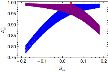
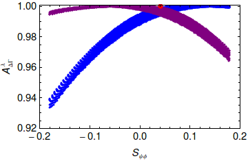
8.5 A Brief Look at the Small Oases

We will now briefly discuss the small oases. It turns out that they correspond to NP contributions to $M_{12}^{d}$ and $M_{12}^{s}$ that are roughly by a factor of two larger than their SM values but carry opposite signs. As $\Delta M_{d,s}$ involve the absolute values of the mixing amplitudes these oases cannot be eliminated on the basis of them. The situation is analogous to the sign of the Wilson coefficient $C_{7\gamma}$ that cannot be fixed by $B\to X_{s}\gamma$ decay. To this end other observables have to be invoked and this is what we will do now in the case at hand.

We anticipated that among the 16 possible oases obtained when the two pairs of parameters $({\tilde{s}}_{23},\delta_{2})$ and $({\tilde{s}}_{13},\delta_{1})$ belong to the regions denoted by $A_{i}$ and $B_{i}$ ( $i=1,\dots 4$ ) in Tables 5 and 6, respectively, it possible to rule out the 8 ones obtained when the pair $({\tilde{s}}_{23},\delta_{2})$ belongs either to $A_{2}$ or to $A_{4}$ . This is a consequence of the requirement that $\varepsilon_{K}$ does not differ more than $5\%$ with respect to the experimental central value reported in Table 4, an uncertainty larger than the experimental range reported in the same table. This request is violated when $(\tilde{s}_{23},\delta_{2})$ vary in $A_{2}$ or in $A_{4}$ , allowing us to half the number of possible oases provided the theoretical and parametric uncertainties in $\varepsilon_{K}$ could be lowered down to $5\%$ . This is clearly not the case at present, primarly due to $|V_{cb}|^{4}$ dependence present in $\varepsilon_{K}$ but could become realistic in the second half of this decade.

In the previous subsection we discussed the case of the big oases, i.e. that in which the parameters belong to $A_{i}$ and $B_{i}$ with $i=1,3$ . There are still other 4 possible regions obtained when the parameters $({\tilde{s}}_{13},\delta_{1})$ vary in $B_{2}$ or $B_{4}$ . The resulting combinations of oases are therefore:

(A_{1},B_{2}),\hskip 28.45274pt(A_{1},B_{4}),\hskip 28.45274pt(A_{3},B_{2}),\hskip 28.45274pt(A_{3},B_{4}).\hskip 28.45274pt

(225)

At present we cannot rule out these regions, but from Fig. 7 and 11 we can observe that correlation between $B(B_{d}\to\mu^{+}\mu^{-})$ and $S_{\mu^{+}\mu^{-}}^{s,d}$ can help distinguishing among these four as well as for the big ones. In particular:

•

In $(A_{1},B_{4})$ (gray)

S_{\mu^{+}\mu^{-}}^{s}<0,\hskip 22.99988pt\mathcal{B}(B_{d}\to\mu^{+}\mu^{-})<\mathcal{B}(B_{d}\to\mu^{+}\mu^{-})_{\rm SM},\hskip 22.99988ptS_{\mu^{+}\mu^{-}}^{d}<0.

(226)

•

In $(A_{1},B_{2})$ (red)

S_{\mu^{+}\mu^{-}}^{s}<0,\hskip 22.99988pt\mathcal{B}(B_{d}\to\mu^{+}\mu^{-})>\mathcal{B}(B_{d}\to\mu^{+}\mu^{-})_{\rm SM},\hskip 22.99988ptS_{\mu^{+}\mu^{-}}^{d}>0.

(227)

•

In $(A_{3},B_{4})$ (brown)

S_{\mu^{+}\mu^{-}}^{s}>0,\hskip 22.99988pt\mathcal{B}(B_{d}\to\mu^{+}\mu^{-})<\mathcal{B}(B_{d}\to\mu^{+}\mu^{-})_{\rm SM},\hskip 22.99988ptS_{\mu^{+}\mu^{-}}^{d}<0.

(228)

•

In $(A_{3},B_{2})$ (magenta)

S_{\mu^{+}\mu^{-}}^{s}>0,\hskip 22.99988pt\mathcal{B}(B_{d}\to\mu^{+}\mu^{-})>\mathcal{B}(B_{d}\to\mu^{+}\mu^{-})_{\rm SM},\hskip 22.99988ptS_{\mu^{+}\mu^{-}}^{d}>0.

(229)

However, compared to the big oases, these small oases are special since they give sharp predictions for the branching ratio of $B_{d}\to\mu^{+}\mu^{-}$ decay and this may one day help to rule them out or confirm. We find: $B(B_{d}\to\mu^{+}\mu^{-})=(1.74\pm 0.02)\times 10^{-10}$ in $(A_{1},B_{2})$ and $(A_{3},B_{2})$ while $B(B_{d}\to\mu^{+}\mu^{-})=(0.911\pm 0.005)\times 10^{-10}$ in $(A_{1},B_{4})$ and $(A_{3},B_{4})$ , for $M_{Z^{\prime}}=1$ TeV, and $B(B_{d}\to\mu^{+}\mu^{-})=(1.172\pm 0.005)\times 10^{-10}$ in $(A_{1},B_{2})$ and $(A_{3},B_{2})$ while $B(B_{d}\to\mu^{+}\mu^{-})=(0.892\pm 0.001)\times 10^{-10}$ in $(A_{1},B_{4})$ and $(A_{3},B_{4})$ , for $M_{Z^{\prime}}=3$ TeV. It can also be observed that, in the 3 TeV case there is no more overlap between the small and the big oases.

Finally, we note that the asymmetry $S_{\mu^{+}\mu^{-}}^{d}$ is very precisely predicted in the small oases. For instance at $M_{Z^{\prime}}=1~$ TeV in oases $B_{2}$ and $B_{4}$ , we find for $S_{\mu^{+}\mu^{-}}^{d}=-0.66\pm 0.03$ and $S_{\mu^{+}\mu^{-}}^{d}=-0.38\pm 0.08$ , respectively.

8.6 Deviations from CMFV Relations.

The calculation of the various observables performed in the previous subsection within the $\overline{331}$ model allows us to discuss the departure from CMFV relations, i.e. the deviation of the functions in Eq. (189) from 1. We find that such functions vary in the following ranges when the parameters belong to the big oases:

•

1 TeV

$\displaystyle r(\Delta M)$	$\displaystyle\in$	$\displaystyle[0.88,1.07]$	(230)
$\displaystyle r(\nu\bar{\nu})$	$\displaystyle\in$	$\displaystyle[0.84,1.19]$	(231)
$\displaystyle r(\mu^{+}\mu^{-})$	$\displaystyle\in$	$\displaystyle[0.60,1.62]$	(232)

•

3 TeV

$\displaystyle r(\Delta M)$	$\displaystyle\in$	$\displaystyle[0.88,1.07]$	(233)
$\displaystyle r(\nu\bar{\nu})$	$\displaystyle\in$	$\displaystyle[0.94,1.06]$	(234)
$\displaystyle r(\mu^{+}\mu^{-})$	$\displaystyle\in$	$\displaystyle[0.85,1.18]\,.$	(235)

We observe that deviation of $r(\Delta M)$ from 1 is approximately $10\%$ , irrespective of the value of $M_{Z^{\prime}}$ . $r(\nu\bar{\nu})$ can deviate by almost $20\%$ from 1 in the case $M_{Z^{\prime}}=1$ TeV, while the deviation reduces to $6\%$ for $M_{Z^{\prime}}=3$ TeV. $r(\mu^{+}\mu^{-})$ is by far the function that mostly deviates from CMFV prediction: its values can differ from 1 by $60\%$ for $M_{Z^{\prime}}=1$ TeV, and almost $20\%$ for $M_{Z^{\prime}}=3$ TeV.

The departure of these functions from 1 is anti-correlated in the case of $r(\mu^{+}\mu^{-})$ and $r(\nu\bar{\nu})$ , as can be seen from Fig. 18 from which we argue that when $r(\nu\bar{\nu})>1$ $(<1)$ it implies $r(\mu^{+}\mu^{-})<1$ $(>1)$ . The largest possible values of $r(\nu\bar{\nu})$ are obtained when $({\tilde{s}}_{13},\delta_{1})\in B_{1}$ , while $r(\mu^{+}\mu^{-})$ is larger when $({\tilde{s}}_{13},\delta_{1})\in B_{3}$ .

The case in which the parameters belong to the small oases is not displayed in Fig. 18. However, we mention that in this case, for $M_{Z^{\prime}}=1$ TeV, the values of $r(\nu\bar{\nu})$ can be larger, while $r(\mu^{+}\mu^{-})$ can reach even the value $r(\mu^{+}\mu^{-})=2.2$ in the region $(A_{1},B_{2})$ . For $M_{Z^{\prime}}=3$ TeV the contribution of the small oases is almost indistinguishable from that of the big ones, except that $r(\mu^{+}\mu^{-})$ and $r(\nu\bar{\nu})$ can be as large as 1.3 and 1.1, respectively.

The violation of CMFV relations in the $\overline{331}$ model can be discussed also comparing the actual results for the branching ratios of $B_{d,s}\to\mu^{+}\mu^{-}$ to what one would obtain from Eq. (190) putting $r=1$ . This is done in Fig. 19, where we plot $B(B_{d}\to\mu^{+}\mu^{-})$ vs $B(B_{s}\to\mu^{+}\mu^{-})$ and superimpose the band corresponding to the relation (190) with $r=1$ and including the errors on the experimental determinations of $\Delta M_{s}$ , $\Delta M_{d}$ , $\tau(B_{s})$ , $\tau(B_{d})$ . On the other hand, we used ${\hat{B}_{s}}/{\hat{B}_{d}}=1.05\pm 0.03$ , where the central value coincides with the lattice determination reported in Table 4, while we reduced the size of the uncertainty. An improvement in this direction would indeed substantially help understanding if and how much CMFV relations are violated in the $\overline{331}$ model.

8.7 What if $Z^{\prime}$ is beyond the LHC Reach?

Our numerical analysis assumed that $Z^{\prime}$ will be found at the LHC, that is $M_{Z^{\prime}}$ is somewhere in the range $1-3~$ TeV. In this range the B-physics constraints imply rather small values for $\tilde{s}_{13}$ and $\tilde{s}_{23}$ and consequently for their product that enters $\varepsilon_{K}$ . NP effects in $\varepsilon_{K}$ are then small and $|V_{ub}|$ has to be sufficiently large in order that $\varepsilon_{K}$ is consistent with the data.

But what if $Z^{\prime}$ is beyond the LHC reach and its mass is as large as $10$ TeV? We have analyzed this case with the following result:

•

The increase of $M_{Z^{\prime}}$ to $10$ TeV still allows to satisfy the constraints in (217) and (218) provided the values of $\tilde{s}_{13}$ and $\tilde{s}_{23}$ are appropriately increased (see below).
•

In turn, as already mentioned previously, NP effects in $\varepsilon_{K}$ can be larger so that for $M_{Z^{\prime}}=10$ TeV even the exclusive value for $|V_{ub}|$ allows to reproduce the data for $\varepsilon_{K}$ , which is not possible for the values of $M_{Z^{\prime}}$ in the few TeV range.
•

NP effects in rare B-decays are strongly suppressed relatively to the effects presented by us for $1\,{\rm TeV}\leq M_{Z^{\prime}}\leq 3\,{\rm TeV}$ so that here similarly to rare $K$ decays everything is SM-like.

Thus the main effect of NP in this case in the $\overline{331}$ model is to remove the anomalies in $\Delta F=2$ observables in the presence of exclusive value of $|V_{ub}|$ without basically any impact on rare $B$ and rare $K$ decays. This rather uninteresting vision could become reality if eventually $\mathcal{B}(B^{+}\to\tau^{+}\nu_{\tau})$ will turn out to be SM-like, favouring exclusive value of $|V_{ub}|$ .

We have investigated this case in more detail by setting $|V_{ub}|=3.1\cdot 10^{-3}$ , $M_{Z^{\prime}}=10$ TeV and imposing additional constraint:

0.75\leq\frac{\Delta M_{K}}{(\Delta M_{K})_{\rm SM}}\leq 1.25,\hskip 22.99988pt2.0\times 10^{-3}\leq|\varepsilon_{K}|\leq 2.5\times 10^{-3}.

(236)

This additional constraint is necessary as now NP effects in $\varepsilon_{K}$ for $\tilde{s}_{23}$ and $\tilde{s}_{13}$ allowed by $B$ -physics $\Delta F=2$ observables in the presence of $M_{Z^{\prime}}=10$ TeV can be large. We find then approximately:

0.05\leq\tilde{s}_{23}\leq 0.12,\hskip 22.99988pt0.016\leq\tilde{s}_{13}\leq 0.030

(237)

and the ranges for $\delta_{1,2}$ slightly shifted to lower values. The reason for some departure from the expected $M_{Z^{\prime}}$ dependence in the range discussed until now is the additional constraint in (236) which is immaterial for $M_{Z^{\prime}}$ of a few TeV.

The fact that maximal values of $\varepsilon_{K}$ increase with $M_{Z^{\prime}}$ when only B-physics constraints are taken into account is related to the increase of $\tilde{s}_{23}$ and $\tilde{s}_{13}$ as already explained. But when the $\Delta^{sd}(Z^{\prime})$ reaches its maximal value, further increase of $M_{Z^{\prime}}$ will also decrease NP contributions to $\varepsilon_{K}$ so that for very large $M_{Z^{\prime}}$ SM results are obtained as required by decoupling of NP. However, this happens only for $M_{Z^{\prime}}\geq 3000$ TeV. This result is just a confirmation of the known fact that if the FCNC $Z^{\prime}$ couplings to quarks are $\mathcal{O}(1)$ , $\varepsilon_{K}$ puts a very strong constraint on the scale of NP.

8.8 Sensitivity to Non-Perturbative Parameters

In the present paper we have used the most recent lattice input to find out that the SM values for $\Delta M_{s}$ and $\Delta M_{d}$ were visibly above the data, when the hadronic and CKM uncertainties were reduced down to $\pm 5\%$ . Here we would like to emphasize that some of the correlations presented by us would change if $\Delta M_{s}$ and $\Delta M_{d}$ would both be found below the data. In order to illustrate this point we have reduced the values of $\hat{B}_{B_{q}}$ by $20\%$ so that now

(\Delta M_{s})_{\rm SM}=15.2~{\rm ps}^{-1},\hskip 11.49994pt(\Delta M_{d})_{\rm SM}=0.45~{\rm ps}^{-1}.

(238)

This result would be welcomed by CMFV models in which $\Delta M_{s}$ and $\Delta M_{d}$ can only be enhanced keeping their ratio fixed. However, the enhanced value of $S_{\psi K_{S}}$ in the large $|V_{ub}|$ scenario still would be problematic for these models.

The $\overline{331}$ model faces this new situation as follows. It chooses the phases $\delta_{1}$ and $\delta_{2}$ , dependently on the oasis considered close to $0^{\circ}$ or $180^{\circ}$ . For $B_{d}$ system we find:

-12^{\circ}\leq\delta_{2}\leq 12^{\circ}\hskip 11.49994pt({\rm green}),\hskip 22.99988pt167^{\circ}\leq\delta_{2}\leq 192^{\circ}\hskip 11.49994pt({\rm yellow})

(239)

with $0.0023\leq\tilde{s}_{13}\leq 0.0036$ . For $B_{s}$ system we find:

-30^{\circ}\leq\delta_{2}\leq 35^{\circ}\hskip 11.49994pt({\rm purple}),\hskip 22.99988pt150^{\circ}\leq\delta_{2}\leq 215^{\circ}\hskip 11.49994pt({\rm blue})

(240)

with $0.01\leq\tilde{s}_{23}\leq 0.019$ .

In both cases $\Delta M_{s}$ and $\Delta M_{d}$ being sensitive to $2\delta_{i}$ are enhanced. In the case of $B_{s}^{0}-\bar{B}_{s}^{0}$ system, where the $S_{\psi\phi}$ asymmetry is small both in the SM and data, the apperance of a small $2\delta_{2}$ is rather natural. In the case of $B_{d}^{0}-\bar{B}_{d}^{0}$ system the addition of a new contribution with a new phase much smaller than the SM phase lowers $S_{\psi K_{S}}$ through the interference of both contributions, as desired.

The question then arises what impact does this new structure have on correlations presented above. Setting $M_{Z^{\prime}}=1\,{\rm TeV}$ we answer this question in Figs. 20 and 21 for most interesting correlations. We observe:

•

As seen in Fig. 20 in the $B_{d}$ meson system, the general structure of correlations is unchanged but the NP effects this time in $B_{d}\to\mu^{+}\mu^{-}$ are found to be much larger than in $S^{d}_{\mu^{+}\mu^{-}}$ .
•

As seen in Fig. 21 the impact on the $B_{s}$ system is much larger. Now the roles of $B_{s}\to\mu^{+}\mu^{-}$ and $S^{s}_{\mu^{+}\mu^{-}}$ in the search for optimal oasis are interchanged. The suppressions or enhancements of $\mathcal{B}(B_{s}\to\mu^{+}\mu^{-})$ relatively to the SM uniquely identify the optimal oasis. Moreover, $\mathcal{B}(B_{s}\to\mu^{+}\mu^{-})$ is bound to be different from the SM values. $S^{s}_{\mu^{+}\mu^{-}}$ can now be vanishing and can only identify the optimal oasis in combination with $S_{\psi\phi}$ , moreover it is now significantly smaller than previously.

This analysis demonstrates clearly that it is crucial the have precise determinations of flavour observables within the SM in order to be able to search indirectly for NP.

9 Summary

In this paper we have reconsidered the flavour structure of the 331 models concentrating the phenomenology on a particular model, the $\overline{331}$ model. In this model the dominant NP contributions come from $Z^{\prime}$ tree-level exchanges. For $M_{Z^{\prime}}$ of order of few TeV, visible departures from the SM expectations are possible. As a detailed analysis of phenomenological implications and related correlations have been presented in the previous section we only list few highlights:

•

Favouring the inclusive value of $|V_{ub}|$ , for $1\,{\rm TeV}\leq M_{Z^{\prime}}\leq 3\,{\rm TeV}$ , the $\overline{331}$ model agrees well with the most recent $B^{+}\to\tau^{+}\nu_{\tau}$ data, removes the $\varepsilon_{K}-S_{\psi K_{S}}$ tension present in the SM and the $\varepsilon_{K}-\Delta M_{s,d}$ tension present in CMFV models. Simultaneously, while differing from the SM, it is consistent with the present data on $B_{s,d}\to\mu^{+}\mu^{-}$ and $S_{\psi\phi}$ .
•

We identify four big oases in the parameter space that can be uniquely distinguished by the values of $\mathcal{B}(B_{d}\to\mu^{+}\mu^{-})$ and $S_{\mu^{+}\mu^{-}}^{s}$ . Also the asymmetry $S_{\mu^{+}\mu^{-}}^{d}$ is helpful in this respect.
•

In each oasis there is a definite correlation between $\mathcal{B}(B_{s}\to\mu^{+}\mu^{-})$ and $S_{\psi\phi}$ so that also these two variables, when considered simultaneously can give valuable information about the model.
•

There are also four oases that cannot be ruled out at present but as predictions for various observables are very sharp in these oases, it is likely that they will not survive more precise data.
•

A characteristic feature of the model is the anti-correlation between $\mathcal{B}(B_{s}\to\mu^{+}\mu^{-})$ and $\mathcal{B}(B\to X_{s}\nu\bar{\nu})$ .
•

$Z^{\prime}$ contributions to $b\to s\nu\bar{\nu}$ transitions, $K^{+}\rightarrow\pi^{+}\nu\bar{\nu}$ and $K_{L}\rightarrow\pi^{0}\nu\bar{\nu}$ are found typically below $5-10\%$ .
•

The violation of CMFV relations are clearly visible with the largest one related to $B_{s,d}\to\mu^{+}\mu^{-}$ decays.
•

We have investigated the case of $M_{Z^{\prime}}=10$ TeV, demonstrating that for such high values of $Z^{\prime}$ mass the pattern of departures from the SM changes, allowing to remove all anomalies even for exclusive values of $|V_{ub}|$ . But then NP effects in rare $B$ and $K$ decays are very small.

We are aware of the fact that some of the correlations presented by us would be washed out if we included all existing uncertainties. Yet, our simplified numerical analysis had as the main goal to illustrate how the decrease of theoretical, parametric and experimental uncertainties in the coming years might allow to exhibit certain features of NP, even if the deviations from the SM will be only moderate. In fact within the coming years the size of the assumed uncetainties in our analysis could likely become reality.

The correlations between various observables found in this paper will allow to distinguish it from other simple secenarios. In particular we have demonstrated that sizable violation of CMFV relations are still possible in this model. Here we would like to make a brief comparision of the $\overline{331}$ model with the ${\rm 2HDM_{\overline{MFV}}}$ and $MU(2)^{3}$ models. The most striking differences are as follows:

•

${\rm 2HDM_{\overline{MFV}}}$ [105] and $\overline{331}$ model share the property that the NP contributions to $\varepsilon_{K}$ are small favouring thereby inclusive value of $|V_{ub}|$ . In ${\rm 2HDM_{\overline{MFV}}}$ , the data on $S_{\psi K_{S}}$ imply then automatically a positive value of $S_{\psi\phi}\geq 0.15$ [2]. In $\overline{331}$ model this is not required and any value within the LHCb range is still possible. Concerning $\Delta F=1$ transitions let us just mention that in ${\rm 2HDM_{\overline{MFV}}}$ there is some tendency that with increasing $S_{\psi\phi}$ also the lower bound on $\mathcal{B}(B_{s}\to\mu^{+}\mu^{-})$ increases. In $\overline{331}$ model, as seen in Fig. 12, the correlation $S_{\psi\phi}-\mathcal{B}(B_{s}\to\mu^{+}\mu^{-})$ is much more transparent. Moreover, while in the oasis $A_{1}$ these two observables are correlated, they are anti-correlated in the oasis $A_{3}$ . In both models $\mathcal{B}(B_{s}\to\mu^{+}\mu^{-})$ can be smaller and larger than the SM value, but in ${\rm 2HDM_{\overline{MFV}}}$ the deviations can be larger, a characteristic property of scalar currents.
•

In the case of $MU(2)^{3}$ models, the most striking differences from the $\overline{331}$ model are the correlation $S_{\psi K_{S}}-S_{\psi\phi}-|V_{ub}|$ [14] that is absent in the $\overline{331}$ model and the fact that $MU(2)^{3}$ models can be made consistent with the FCNC data for exclusive value of $|V_{ub}|$ , while this is rather difficult in the $\overline{331}$ model for $M_{Z^{\prime}}\leq 5\,{\rm TeV}$ . Finding in the future that exclusive value for $|V_{ub}|$ is chosen by nature and $M_{Z^{\prime}}\leq 5\,{\rm TeV}$ would favour $MU(2)^{3}$ models over $\overline{331}$ model. On the other hand if the inclusive value of $|V_{ub}|$ is the right one and $S_{\psi\phi}$ is found to be negative, this would put $MU(2)^{3}$ models into difficulties while the $\overline{331}$ model would face such data without any problems.

In view of these definite findings we are looking forward to improved experimental data and improved lattice calculations. The plots presented by us should facilitate monitoring the future confrontations of the $\overline{331}$ model with the data and to find out whether this simple model can satisfactorily describe the observables considered by us.

The generalization of our analysis to $Z^{\prime}$ models with both right-handed and left-handed couplings and sizable NP contributions to $\varepsilon_{K}$ and rare $K$ decays is presented in [106].

Acknowledgments

We would like to thank Pietro Colangelo and Robert Fleischer for discussions. This research was done and financed in the context of the ERC Advanced Grant project “FLAVOUR”(267104) and was partially supported by the DFG cluster of excellence “Origin and Structure of the Universe”.

Appendix A Appendix

We collect the formulae for the couplings of $Z^{\prime}$ to quarks and leptons especially for $\beta=\sqrt{3}$ and $\frac{1}{\sqrt{3}}$ that enter various expressions in our paper.

Case 1: arbitrary $\beta$


$\displaystyle\Delta_{L}^{ij}(Z^{\prime})$	$\displaystyle=\frac{g}{\sqrt{3}c_{W}\sqrt{1-(1+\beta^{2})s_{W}^{2}}}c_{W}^{2}v_{3i}^{*}v_{3j}\,,$	(241a)
$\displaystyle\Delta_{L}^{ji}(Z^{\prime})$	$\displaystyle=\left[\Delta_{L}^{ij}(Z^{\prime})\right]^{\star}\,,$	(241b)
$\displaystyle\Delta_{L}^{\nu\bar{\nu}}(Z^{\prime})$	$\displaystyle=\frac{g~\left[1-(1+\sqrt{3}\beta)s_{W}^{2}\right]}{2\sqrt{3}c_{W}\sqrt{1-(1+\beta^{2})s_{W}^{2}}}\,,$	(241c)
$\displaystyle\Delta_{L}^{\mu\bar{\mu}}(Z^{\prime})$	$\displaystyle=\Delta_{L}^{\nu\bar{\nu}}(Z^{\prime})\,,$	(241d)
$\displaystyle\Delta_{R}^{\mu\bar{\mu}}(Z^{\prime})$	$\displaystyle=\left\{\begin{array}[]{cc}\frac{-g~\beta~s_{W}^{2}}{c_{W}\sqrt{1-(1+\beta^{2})s_{W}^{2}}}\,,&\hskip 11.49994pt\beta\neq\sqrt{3}\\ \frac{g\sqrt{1-4s_{W}^{2}}}{\sqrt{3}c_{W}}\,,&\hskip 11.49994pt\beta=\sqrt{3}\\ \end{array}\right.$

Case 2: $\beta=\sqrt{3}$


$\displaystyle\Delta_{L}^{sd}(Z^{\prime})$	$\displaystyle=\frac{g}{\sqrt{3}c_{W}\sqrt{1-4s_{W}^{2}}}c_{W}^{2}v_{32}^{*}v_{31}=1.84~g\tilde{s}_{13}\tilde{s}_{23}\tilde{c}_{13}e^{i(\delta_{2}-\delta_{1})}\,,$	(242a)
$\displaystyle\Delta_{L}^{bd}(Z^{\prime})$	$\displaystyle=\frac{g}{\sqrt{3}c_{W}\sqrt{1-4s_{W}^{2}}}c_{W}^{2}v_{33}^{*}v_{31}=-1.84~g\tilde{s}_{13}\tilde{c}_{13}\tilde{c}_{23}e^{-i\delta_{1}}\,,$	(242b)
$\displaystyle\Delta_{L}^{bs}(Z^{\prime})$	$\displaystyle=\frac{g}{\sqrt{3}c_{W}\sqrt{1-4s_{W}^{2}}}c_{W}^{2}v_{33}^{*}v_{32}=-1.84~g\tilde{s}_{23}\tilde{c}^{2}_{13}\tilde{c}_{23}e^{-i\delta_{2}}\,,$	(242c)
$\displaystyle\Delta_{L}^{\nu\bar{\nu}}(Z^{\prime})$	$\displaystyle=\frac{g\sqrt{1-4s_{W}^{2}}}{2\sqrt{3}c_{W}}=0.090~g\,,$	(242d)
$\displaystyle\Delta_{L}^{\mu\bar{\mu}}(Z^{\prime})$	$\displaystyle=\frac{1}{2}\Delta_{R}^{\mu\bar{\mu}}(Z^{\prime})=\Delta_{L}^{\nu\bar{\nu}}(Z^{\prime})=\Delta_{A}^{\mu\bar{\mu}}(Z^{\prime})\,,$	(242e)
$\displaystyle\Delta_{V}^{\mu\bar{\mu}}(Z^{\prime})$	$\displaystyle=0.271~g\,.$	(242f)

Case 3: $\beta=\frac{1}{\sqrt{3}}$


$\displaystyle\Delta_{L}^{sd}(Z^{\prime})$	$\displaystyle=\frac{g}{\sqrt{3}c_{W}\sqrt{1-\frac{4}{3}s_{W}^{2}}}c_{W}^{2}v_{32}^{*}v_{31}=0.61~g\tilde{s}_{13}\tilde{s}_{23}\tilde{c}_{13}e^{i(\delta_{2}-\delta_{1})}\,,$	(243a)
$\displaystyle\Delta_{L}^{bd}(Z^{\prime})$	$\displaystyle=\frac{g}{\sqrt{3}c_{W}\sqrt{1-\frac{4}{3}s_{W}^{2}}}c_{W}^{2}v_{33}^{*}v_{31}=-0.61~g\tilde{s}_{13}\tilde{c}_{13}\tilde{c}_{23}e^{-i\delta_{1}}\,,$	(243b)
$\displaystyle\Delta_{L}^{bs}(Z^{\prime})$	$\displaystyle=\frac{g}{\sqrt{3}c_{W}\sqrt{1-\frac{4}{3}s_{W}^{2}}}c_{W}^{2}v_{33}^{*}v_{32}=-0.61~g\tilde{s}_{23}\tilde{c}^{2}_{13}\tilde{c}_{23}e^{-i\delta_{2}}\,,$	(243c)
$\displaystyle\Delta_{L}^{\nu\bar{\nu}}(Z^{\prime})$	$\displaystyle=\frac{g\,\left(1-2s_{W}^{2}\right)}{2\sqrt{3}c_{W}\sqrt{1-\frac{4}{3}s_{W}^{2}}}=0.213~g\,,$	(243d)
$\displaystyle\Delta_{L}^{\mu\bar{\mu}}(Z^{\prime})$	$\displaystyle=\Delta_{L}^{\nu\bar{\nu}}(Z^{\prime})\,,$	(243e)
$\displaystyle\Delta_{R}^{\mu\bar{\mu}}(Z^{\prime})$	$\displaystyle=-\frac{g\,s_{W}^{2}}{\sqrt{3}c_{W}\sqrt{1-\frac{4}{3}s_{W}^{2}}}=\frac{2s_{W}^{2}}{1-2s_{W}^{2}}\Delta_{L}^{\mu\bar{\mu}}(Z^{\prime})=-0.183~g\,$	(243f)
$\displaystyle\Delta_{A}^{\mu\bar{\mu}}(Z^{\prime})$	$\displaystyle=-0.396~g\,,$	(243g)
$\displaystyle\Delta_{V}^{\mu\bar{\mu}}(Z^{\prime})$	$\displaystyle=0.030~g\,.$	(243h)

References

[1] LHCb collaboration Collaboration, I. Bediaga et. al., Implications of LHCb measurements and future prospects, arXiv:1208.3355.
[2] A. J. Buras and J. Girrbach, BSM models facing the recent LHCb data: A First look, Acta Phys.Polon. B43 (2012) 1427, [arXiv:1204.5064].
[3] UTfit Collaboration Collaboration, M. Bona et. al., Model-independent constraints on $\Delta$ F=2 operators and the scale of new physics, JHEP 0803 (2008) 049, [arXiv:0707.0636].
[4] A. Lenz, U. Nierste, J. Charles, S. Descotes-Genon, H. Lacker, et. al., Constraints on new physics in $B-\bar{B}$ mixing in the light of recent LHCb data, Phys.Rev. D86 (2012) 033008, [arXiv:1203.0238].
[5] F. Beaujean, C. Bobeth, D. van Dyk, and C. Wacker, Bayesian Fit of Exclusive $b\to s\bar{\ell}\ell$ Decays: The Standard Model Operator Basis, JHEP 1208 (2012) 030, [arXiv:1205.1838].
[6] S. Descotes-Genon, J. Matias, M. Ramon, and J. Virto, Implications from clean observables for the binned analysis of $B\to K*\mu^{+}\mu^{-}$ at large recoil, arXiv:1207.2753.
[7] R. Barbieri, G. Isidori, J. Jones-Perez, P. Lodone, and D. M. Straub, U(2) and Minimal Flavour Violation in Supersymmetry, Eur.Phys.J. C71 (2011) 1725, [arXiv:1105.2296].
[8] W. Altmannshofer, P. Paradisi, and D. M. Straub, Model-Independent Constraints on New Physics in $b\to s\gamma$ Transitions, JHEP 1204 (2012) 008, [arXiv:1111.1257].
[9] W. Altmannshofer and D. M. Straub, Cornering New Physics in $b\to s\gamma$ Transitions, JHEP 1208 (2012) 121, [arXiv:1206.0273].
[10] F. Botella, G. Branco, and M. Nebot, The Hunt for New Physics in the Flavour Sector with up vector-like quarks, arXiv:1207.4440.
[11] C. Davies, Standard Model Heavy Flavor physics on the Lattice, PoS LATTICE2011 (2011) 019, [arXiv:1203.3862].
[12] C. Tarantino, Flavor Lattice QCD in the Precision Era, arXiv:1210.0474.
[13] M. Bona et. al., SuperB: A High-Luminosity Asymmetric e+ e- Super Flavor Factory. Conceptual Design Report, arXiv:0709.0451.
[14] A. J. Buras and J. Girrbach, On the Correlations between Flavour Observables in Minimal $U(2)^{3}$ Models, arXiv:1206.3878.
[15] A. J. Buras, P. Gambino, M. Gorbahn, S. Jager, and L. Silvestrini, Universal unitarity triangle and physics beyond the standard model, Phys. Lett. B500 (2001) 161–167, [hep-ph/0007085].
[16] G. D’Ambrosio, G. F. Giudice, G. Isidori, and A. Strumia, Minimal flavour violation: An effective field theory approach, Nucl. Phys. B645 (2002) 155–187, [hep-ph/0207036].
[17] A. J. Buras, Minimal flavor violation, Acta Phys. Polon. B34 (2003) 5615–5668, [hep-ph/0310208].
[18] A. J. Buras, Minimal flavour violation and beyond: Towards a flavour code for short distance dynamics, Acta Phys.Polon. B41 (2010) 2487–2561, [arXiv:1012.1447].
[19] F. Pisano and V. Pleitez, An SU(3) x U(1) model for electroweak interactions, Phys.Rev. D46 (1992) 410–417, [hep-ph/9206242].
[20] P. H. Frampton, Chiral dilepton model and the flavor question, Phys. Rev. Lett. 69 (1992) 2889–2891.
[21] M. Blanke et. al., Rare and CP-violating $K$ and $B$ decays in the Littlest Higgs model with T-parity, JHEP 01 (2007) 066, [hep-ph/0610298].
[22] C. Promberger, S. Schatt, and F. Schwab, Flavor Changing Neutral Current Effects and CP Violation in the Minimal 3-3-1 Model, Phys.Rev. D75 (2007) 115007, [hep-ph/0702169].
[23] C. Promberger, S. Schatt, F. Schwab, and S. Uhlig, Bounding the Minimal 331 Model through the Decay $B\to X_{s}\gamma$ , Phys.Rev. D77 (2008) 115022, [arXiv:0802.0949].
[24] E. Lunghi and A. Soni, Possible Indications of New Physics in $B_{d}$ -mixing and in $\sin(2\beta)$ Determinations, Phys. Lett. B666 (2008) 162–165, [arXiv:0803.4340].
[25] A. J. Buras and D. Guadagnoli, Correlations among new CP violating effects in $\Delta F=2$ observables, Phys. Rev. D78 (2008) 033005, [arXiv:0805.3887].
[26] A. J. Buras and D. Guadagnoli, On the consistency between the observed amount of CP violation in the $K$ and $B_{d}$ -systems within minimal flavor violation, Phys.Rev. D79 (2009) 053010, [arXiv:0901.2056].
[27] E. Lunghi and A. Soni, Hints for the scale of new CP-violating physics from B-CP anomalies, JHEP 0908 (2009) 051, [arXiv:0903.5059].
[28] E. Lunghi and A. Soni, Possible evidence for the breakdown of the CKM-paradigm of CP-violation, Phys.Lett. B697 (2011) 323–328, [arXiv:1010.6069].
[29] M. Ciuchini, G. D’Agostini, E. Franco, V. Lubicz, G. Martinelli, et. al., 2000 CKM triangle analysis: A Critical review with updated experimental inputs and theoretical parameters, www.utfit.org, JHEP 0107 (2001) 013, [hep-ph/0012308].
[30] K. De Bruyn, R. Fleischer, R. Knegjens, P. Koppenburg, M. Merk, et. al., Branching Ratio Measurements of $B_{s}$ Decays, Phys.Rev. D86 (2012) 014027, [arXiv:1204.1735].
[31] K. De Bruyn, R. Fleischer, R. Knegjens, P. Koppenburg, M. Merk, et. al., Probing New Physics via the $B^{0}_{s}\to\mu^{+}\mu^{-}$ Effective Lifetime, Phys.Rev.Lett. 109 (2012) 041801, [arXiv:1204.1737].
[32] R. A. Diaz, R. Martinez, and F. Ochoa, The Scalar sector of the SU(3)(c) x SU(3)(L) x U(1)(X) model, Phys.Rev. D69 (2004) 095009, [hep-ph/0309280].
[33] H. N. Long and T. Inami, S, T, U parameters in SU(3)(C) x SU(3)(L) x U(1) model with right-handed neutrinos, Phys.Rev. D61 (2000) 075002, [hep-ph/9902475].
[34] MEG collaboration Collaboration, J. Adam et. al., New limit on the lepton-flavour violating decay $\mu^{+}\to e^{+}\gamma$ , Phys.Rev.Lett. 107 (2011) 171801, [arXiv:1107.5547].
[35] J. T. Liu and D. Ng, Lepton flavor changing processes and CP violation in the 331 model, Phys.Rev. D50 (1994) 548–557, [hep-ph/9401228].
[36] R. A. Diaz, R. Martinez, and F. Ochoa, SU(3)(c) x SU(3)(L) x U(1)(X) models for beta arbitrary and families with mirror fermions, Phys.Rev. D72 (2005) 035018, [hep-ph/0411263].
[37] M. Cvetic and P. Langacker, Implications of Abelian extended gauge structures from string models, Phys.Rev. D54 (1996) 3570–3579, [hep-ph/9511378].
[38] D. Ng, The Electroweak theory of SU(3) x U(1), Phys.Rev. D49 (1994) 4805–4811, [hep-ph/9212284].
[39] J. T. Liu, Generation nonuniversality and flavor changing neutral currents in the 331 model, Phys.Rev. D50 (1994) 542–547, [hep-ph/9312312].
[40] P. Langacker and M. Plumacher, Flavor changing effects in theories with a heavy $Z^{\prime}$ boson with family nonuniversal couplings, Phys.Rev. D62 (2000) 013006, [hep-ph/0001204].
[41] J. A. Rodriguez and M. Sher, FCNC and rare B decays in 3-3-1 models, Phys.Rev. D70 (2004) 117702, [hep-ph/0407248].
[42] J. Agrawal, P. H. Frampton, and J. T. Liu, The Decay $b\to s\gamma$ in the 3-3-1 model, Int.J.Mod.Phys. A11 (1996) 2263–2280, [hep-ph/9502353].
[43] R. Peccei and H. R. Quinn, CP Conservation in the Presence of Instantons, Phys.Rev.Lett. 38 (1977) 1440–1443.
[44] P. B. Pal, The Strong CP question in SU(3)(C) x SU(3)(L) x U(1)(N) models, Phys.Rev. D52 (1995) 1659–1662, [hep-ph/9411406].
[45] M. Blanke et. al., Particle antiparticle mixing, $\varepsilon_{K}$ , $\Delta\Gamma_{q}$ , $A_{\text{SL}}^{q}$ , $A_{\text{CP}}(B_{d}\to\psi K_{S})$ , $A_{\text{CP}}(B_{s}\to\psi\phi)$ and $B\to X_{s,d}\gamma$ in the Littlest Higgs model with T- parity, JHEP 12 (2006) 003, [hep-ph/0605214].
[46] S. Herrlich and U. Nierste, Enhancement of the $K_{L}-K_{S}$ mass difference by short distance QCD corrections beyond leading logarithms, Nucl. Phys. B419 (1994) 292–322, [hep-ph/9310311].
[47] S. Herrlich and U. Nierste, Indirect CP violation in the neutral kaon system beyond leading logarithms, Phys. Rev. D52 (1995) 6505–6518, [hep-ph/9507262].
[48] S. Herrlich and U. Nierste, The Complete $|\Delta S|=2$ Hamiltonian in the Next-To-Leading Order, Nucl. Phys. B476 (1996) 27–88, [hep-ph/9604330].
[49] A. J. Buras, M. Jamin, and P. H. Weisz, Leading and next-to-leading QCD corrections to $\varepsilon$ parameter and $B^{0}-\bar{B}^{0}$ mixing in the presence of a heavy top quark, Nucl. Phys. B347 (1990) 491–536.
[50] J. Urban, F. Krauss, U. Jentschura, and G. Soff, Next-to-leading order QCD corrections for the $B^{0}-\bar{B}^{0}$ mixing with an extended Higgs sector, Nucl. Phys. B523 (1998) 40–58, [hep-ph/9710245].
[51] J. Brod and M. Gorbahn, $\epsilon_{K}$ at Next-to-Next-to-Leading Order: The Charm-Top-Quark Contribution, Phys.Rev. D82 (2010) 094026, [arXiv:1007.0684].
[52] J. Brod and M. Gorbahn, Next-to-Next-to-Leading-Order Charm-Quark Contribution to the CP Violation Parameter $\varepsilon_{K}$ and $\Delta M_{K}$ , Phys.Rev.Lett. 108 (2012) 121801, [arXiv:1108.2036].
[53] A. J. Buras and J. Girrbach, Complete NLO QCD Corrections for Tree Level Delta F = 2 FCNC Processes, JHEP 1203 (2012) 052, [arXiv:1201.1302].
[54] A. J. Buras, S. Jager, and J. Urban, Master formulae for $\Delta F=2$ NLO QCD factors in the standard model and beyond, Nucl.Phys. B605 (2001) 600–624, [hep-ph/0102316].
[55] A. J. Buras, D. Guadagnoli, and G. Isidori, On $\epsilon_{K}$ beyond lowest order in the Operator Product Expansion, Phys.Lett. B688 (2010) 309–313, [arXiv:1002.3612].
[56] UTfit Collaboration, M. Bona et. al., The UTfit collaboration report on the status of the unitarity triangle beyond the standard model. I: Model- independent analysis and minimal flavour violation, JHEP 03 (2006) 080, [hep-ph/0509219].
[57] G. Buchalla and A. J. Buras, The rare decays $k\to\pi\nu\bar{\nu}$ , $b\to x\nu\bar{\nu}$ and $b\to\ell^{+}\ell^{-}$ : An update, Nucl. Phys. B548 (1999) 309–327, [hep-ph/9901288].
[58] A. J. Buras, M. Gorbahn, U. Haisch, and U. Nierste, The rare decay $K^{+}\to\pi^{+}\nu\bar{\nu}$ at the next-to-next-to-leading order in QCD, Phys. Rev. Lett. 95 (2005) 261805, [hep-ph/0508165].
[59] A. J. Buras, M. Gorbahn, U. Haisch, and U. Nierste, Charm quark contribution to $K^{+}\to\pi^{+}\nu\bar{\nu}$ at next-to-next-to-leading order, JHEP 11 (2006) 002, [hep-ph/0603079].
[60] J. Brod and M. Gorbahn, Electroweak Corrections to the Charm Quark Contribution to $K^{+}\to\pi^{+}\nu\bar{\nu}$ , Phys. Rev. D78 (2008) 034006, [arXiv:0805.4119].
[61] J. Brod, M. Gorbahn, and E. Stamou, Two-Loop Electroweak Corrections for the $K\to\pi\nu\bar{nu}$ Decays, Phys.Rev. D83 (2011) 034030, [arXiv:1009.0947].
[62] M. Misiak and J. Urban, QCD corrections to FCNC decays mediated by Z penguins and W boxes, Phys.Lett. B451 (1999) 161–169, [hep-ph/9901278].
[63] A. J. Buras, L. Merlo, and E. Stamou, The Impact of Flavour Changing Neutral Gauge Bosons on $\bar{B}\to X_{s}\gamma$ , JHEP 1108 (2011) 124, [arXiv:1105.5146].
[64] M. Misiak, H. Asatrian, K. Bieri, M. Czakon, A. Czarnecki, et. al., Estimate of $\mathcal{B}(\bar{B}\to X(s)\gamma)$ at $\mathcal{O}(\alpha_{s}^{2})$ , Phys.Rev.Lett. 98 (2007) 022002, [hep-ph/0609232].
[65] P. L. Cho and M. Misiak, $b\to s\gamma$ decay in $SU(2)_{L}\times SU(2)_{R}\times U(1)$ extensions of the Standard Model, Phys.Rev. D49 (1994) 5894–5903, [hep-ph/9310332].
[66] M. Blanke, A. J. Buras, K. Gemmler, and T. Heidsieck, $\Delta F=2$ observables and $B\to X_{q}\gamma$ ; in the Left-Right Asymmetric Model: Higgs particles striking back, JHEP 1203 (2012) 024, [arXiv:1111.5014].
[67] A. J. Buras, F. Schwab, and S. Uhlig, Waiting for precise measurements of $K^{+}\to\pi^{+}\nu\bar{\nu}$ and $K_{L}\to\pi^{0}\nu\bar{\nu}$ , Rev. Mod. Phys. 80 (2008) 965–1007, [hep-ph/0405132].
[68] G. Isidori, Flavor Physics with light quarks and leptons, eConf C060409 (2006) 035, [hep-ph/0606047].
[69] C. Smith, Theory review on rare K decays: Standard model and beyond, hep-ph/0608343.
[70] F. Mescia and C. Smith, Improved estimates of rare K decay matrix-elements from $K_{\ell 3}$ decays, Phys. Rev. D76 (2007) 034017, [arXiv:0705.2025].
[71] G. Isidori, F. Mescia, and C. Smith, Light-quark loops in $K\to\pi\nu\bar{\nu}$ , Nucl. Phys. B718 (2005) 319–338, [hep-ph/0503107].
[72] W. Altmannshofer, A. J. Buras, D. M. Straub, and M. Wick, New strategies for New Physics search in $B\to K^{*}\nu\bar{\nu}$ , $B\to K\nu\bar{\nu}$ and $B\to X_{s}\nu\bar{\nu}$ decays, JHEP 04 (2009) 022, [arXiv:0902.0160].
[73] J. F. Kamenik and C. Smith, Tree-level contributions to the rare decays $B^{+}\to\pi^{+}\nu\bar{\nu},B^{+}\to K^{+}\nu\bar{\nu}$ , and $B^{+}\to K^{*+}\nu\bar{\nu}$ in the Standard Model, Phys.Lett. B680 (2009) 471–475, [arXiv:0908.1174].
[74] M. Bartsch, M. Beylich, G. Buchalla, and D.-N. Gao, Precision Flavour Physics with $B\to K\nu\bar{\nu}$ and $B\to Kl^{+}l^{-}$ , JHEP 0911 (2009) 011, [arXiv:0909.1512].
[75] ALEPH Collaboration, R. Barate et. al., Measurements of $BR(b\to\tau^{-}\bar{\nu}_{\tau}X)$ and $BR(b\to\tau^{-}\bar{\nu}_{\tau}D^{*\pm}X)$ and upper limits on $BR(B^{-}\to\tau^{-}\bar{\nu}_{\tau})$ and $BR(b\to\nu\bar{\nu})$ , Eur. Phys. J. C19 (2001) 213–227, [hep-ex/0010022].
[76] BELLE Collaboration, K. F. Chen et. al., Search for $B\to h^{(*)}\nu\bar{\nu}$ Decays at Belle, Phys. Rev. Lett. 99 (2007) 221802, [arXiv:0707.0138].
[77] BABAR Collaboration, B. Aubert et. al., Search for $B\to K^{*}\nu\bar{\nu}$ decays, Phys. Rev. D78 (2008) 072007, [arXiv:0808.1338].
[78] S. Descotes-Genon, J. Matias, and J. Virto, An analysis of $B_{d,s}$ mixing angles in presence of New Physics and an update of $B_{s}\to$ K0* anti-K0*, Phys.Rev. D85 (2012) 034010, [arXiv:1111.4882].
[79] A. J. Buras, J. Girrbach, D. Guadagnoli, and G. Isidori, On the Standard Model prediction for $\mathcal{B}(B_{s,d}\to\mu^{+}\mu^{-})$ , arXiv:1208.0934.
[80] R. Fleischer, On Branching Ratios of $B_{s}$ Decays and the Search for New Physics in $B^{0}_{s}\to\mu^{+}\mu^{-}$ , arXiv:1208.2843.
[81] A. J. Buras, R. Fleischer, S. Recksiegel, and F. Schwab, Anatomy of prominent $B$ and $K$ decays and signatures of CP-violating new physics in the electroweak penguin sector, Nucl. Phys. B697 (2004) 133–206, [hep-ph/0402112].
[82] M. Gorbahn and U. Haisch, Charm quark contribution to $K_{L}\to\mu^{+}\mu^{-}$ at next-to-next-to-leading order, Phys. Rev. Lett. 97 (2006) 122002, [hep-ph/0605203].
[83] G. Isidori and R. Unterdorfer, On the short-distance constraints from $K_{L,S}\to\mu^{+}\mu^{-}$ , JHEP 01 (2004) 009, [hep-ph/0311084].
[84] UTfit Collaboration Collaboration, M. Bona et. al., An Improved Standard Model Prediction Of $BR(B\to\tau\nu)$ And Its Implications For New Physics, Phys.Lett. B687 (2010) 61–69, [arXiv:0908.3470].
[85] W. Altmannshofer, A. J. Buras, S. Gori, P. Paradisi, and D. M. Straub, Anatomy and Phenomenology of FCNC and CPV Effects in SUSY Theories, Nucl.Phys. B830 (2010) 17–94, [arXiv:0909.1333].
[86] A. Lenz, U. Nierste, J. Charles, S. Descotes-Genon, A. Jantsch, et. al., Anatomy of New Physics in $B-\bar{B}$ mixing, Phys.Rev. D83 (2011) 036004, [arXiv:1008.1593].
[87] BABAR Collaboration Collaboration, B. Aubert et. al., A Search for $B^{+}\to\tau^{+}\nu$ with Hadronic $B$ tags, Phys.Rev. D77 (2008) 011107, [arXiv:0708.2260].
[88] Belle Collaboration Collaboration, K. Ikado et. al., Evidence of the Purely Leptonic Decay $B^{-}\to\tau^{-}\bar{\nu}_{\tau}$ , Phys.Rev.Lett. 97 (2006) 251802, [hep-ex/0604018].
[89] Particle Data Group Collaboration, K. Nakamura et. al., Review of particle physics, J.Phys.G G37 (2010) 075021.
[90] BABAR Collaboration Collaboration, J. Lees et. al., Evidence of $B\to\tau\nu$ decays with hadronic $B$ tags, arXiv:1207.0698.
[91] Belle Collaboration Collaboration, I. Adachi et. al., Measurement of $b\to\tau\nu$ with a hadronic tagging method using the full data sample of belle, arXiv:1208.4678.
[92] A. J. Buras, Relations between $\Delta M_{s,d}$ and $B_{s,d}\to\mu^{+}\mu^{-}$ in models with minimal flavour violation, Phys. Lett. B566 (2003) 115–119, [hep-ph/0303060].
[93] HPQCD Collaboration Collaboration, J. Shigemitsu et. al., Recent results on B mixing and decay constants from HPQCD, PoS LAT2009 (2009) 251, [arXiv:0910.4131].
[94] J. Laiho, E. Lunghi, and R. S. Van de Water, Lattice QCD inputs to the CKM unitarity triangle analysis, Phys. Rev. D81 (2010) 034503, [arXiv:0910.2928]. Updates available on http://latticeaverages.org/.
[95] P. Clarke, Results on cp violation in $b_{s}$ mixing, . http://cdsweb.cern.ch/record/1429149/files/LHCb-TALK-2012-029.pdf.
[96] LHCb collaboration Collaboration, R. Aaij et. al., Strong constraints on the rare decays $B_{s}\to\mu^{+}\mu^{-}$ and $B^{0}\to\mu^{+}\mu^{-}$ , arXiv:1203.4493.
[97] LHCb collaboration Collaboration, R. Aaij et. al., First evidence for the decay $B_{s}\to\mu^{+}\mu^{-}$ , arXiv:1211.2674.
[98] G. Ricciardi, Brief review on semileptonic B decays, arXiv:1209.1407.
[99] M. Blanke and A. J. Buras, Lower bounds on $\Delta M_{s,d}$ from constrained minimal flavour violation, JHEP 0705 (2007) 061, [hep-ph/0610037].
[100] W. Altmannshofer and D. M. Straub, Cornering New Physics in $b\to s\gamma$ Transitions, JHEP 1208 (2012) 121, [arXiv:1206.0273].
[101] K. Chetyrkin, J. Kuhn, A. Maier, P. Maierhofer, P. Marquard, et. al., Charm and Bottom Quark Masses: An Update, Phys.Rev. D80 (2009) 074010, [arXiv:0907.2110].
[102] HPQCD Collaboration Collaboration, I. Allison et. al., High-Precision Charm-Quark Mass from Current-Current Correlators in Lattice and Continuum QCD, Phys.Rev. D78 (2008) 054513, [arXiv:0805.2999].
[103] Heavy Flavor Averaging Group Collaboration, D. Asner et. al., Averages of $b$ -hadron, $c$ -hadron, and $\tau$ -lepton Properties, arXiv:1010.1589. Long author list - awaiting processing.
[104] CMS Collaboration Collaboration, S. Chatrchyan et. al., Search for narrow resonances in dilepton mass spectra in $pp$ collisions at $\sqrt{s}=7$ TeV, Phys.Lett. B714 (2012) 158–179, [arXiv:1206.1849].
[105] A. J. Buras, M. V. Carlucci, S. Gori, and G. Isidori, Higgs-mediated FCNCs: Natural Flavour Conservation vs. Minimal Flavour Violation, JHEP 1010 (2010) 009, [arXiv:1005.5310].
[106] A. J. Buras, F. De Fazio, and J. Girrbach, The Anatomy of Z’ and Z with Flavour Changing Neutral Currents in the Flavour Precision Era, arXiv:1211.1896.

Abstract

1 Introduction

2 Flavour Structure of the 331 Models

2.1 Preliminaries

2.2 The Model

2.2.1 Gauge Bosons

2.2.2 Fermions

2.2.3 Higgs sector

2.2.4 Masses of the gauge bosons.

2.2.5 Yukawa Lagrangian and interaction Lagrangian terms in their final form.

3 𝚫​𝑭=𝟐\Delta F=2 Transitions

3.1 Preliminaries

3.2 Standard Model Results

3.3 Tree Level 𝒁′Z^{\prime} Contributions

3.4 New Box Contributions

3.5 Basic formulae for 𝚫​𝑭=𝟐\Delta F=2 observables

4 Effective Hamiltonians for 𝚫​𝑭=𝟏\Delta F=1 Decays

4.1 Preliminaries

4.2 Effective Hamiltonian for 𝒔¯→𝒅¯​𝝂​𝝂¯\bar{s}\to\bar{d}\nu\bar{\nu}

4.3 Effective Hamiltonian for 𝒃→𝒅​𝝂​𝝂¯b\to d\nu\bar{\nu} and 𝒃→𝒔​𝝂​𝝂¯b\to s\nu\bar{\nu}

4.4 Effective Hamiltonian for 𝒃→𝒅​ℓ+​ℓ−b\to d\ell^{+}\ell^{-} and 𝒃→𝒔​ℓ+​ℓ−b\to s\ell^{+}\ell^{-}

4.5 Effective Hamiltonian for the 𝑩→𝑿𝒔​𝜸B\to X_{s}\gamma Decay

4.5.1 Preliminaries

4.5.2 𝒁′Z^{\prime} contribution without QCD Corrections

4.5.3 Final Results including QCD corrections

5 Rare Decays

5.1 𝑲+→𝝅+​𝝂​𝝂¯K^{+}\rightarrow\pi^{+}\nu\bar{\nu} and 𝑲𝑳→𝝅𝟎​𝝂​𝝂¯K_{L}\rightarrow\pi^{0}\nu\bar{\nu}

5.2 𝑩→{𝑿𝒔,𝑲,𝑲∗}​𝝂​𝝂¯B\to\{X_{s},K,K^{*}\}\nu\bar{\nu}

5.3 𝑩𝒅,𝒔→𝝁+​𝝁−B_{d,s}\to\mu^{+}\mu^{-}

5.4 𝑲𝑳→𝝁+​𝝁−K_{L}\to\mu^{+}\mu^{-}

5.5 𝑩+→𝝉+​𝝂B^{+}\to\tau^{+}\nu

5.5.1 Standard Model Results

5.5.2 Result in the 331 Model

6 Breakdown of CMFV Relation in the 331 Model

7 Correlations within 331 Model

7.1 Classification

7.2 Master Relations

7.3 Implications

8 Numerical Analysis

8.1 Recent Data and Anomalies

8.2 Strategy

8.3 Simplified Analysis

8.4 The Search for the Optimal Oasis

8.5 A Brief Look at the Small Oases

8.6 Deviations from CMFV Relations.

8.7 What if 𝒁′Z^{\prime} is beyond the LHC Reach?

8.8 Sensitivity to Non-Perturbative Parameters

9 Summary

Acknowledgments

Appendix A Appendix

References

3 $\Delta F=2$ Transitions

3.3 Tree Level $Z^{\prime}$ Contributions

3.5 Basic formulae for $\Delta F=2$ observables

4 Effective Hamiltonians for $\Delta F=1$ Decays

4.2 Effective Hamiltonian for $\bar{s}\to\bar{d}\nu\bar{\nu}$

4.3 Effective Hamiltonian for $b\to d\nu\bar{\nu}$ and $b\to s\nu\bar{\nu}$

4.4 Effective Hamiltonian for $b\to d\ell^{+}\ell^{-}$ and $b\to s\ell^{+}\ell^{-}$

4.5 Effective Hamiltonian for the $B\to X_{s}\gamma$ Decay

4.5.2 $Z^{\prime}$ contribution without QCD Corrections

5.1 $K^{+}\rightarrow\pi^{+}\nu\bar{\nu}$ and $K_{L}\rightarrow\pi^{0}\nu\bar{\nu}$

5.2 $B\to\{X_{s},K,K^{*}\}\nu\bar{\nu}$

5.3 $B_{d,s}\to\mu^{+}\mu^{-}$

5.4 $K_{L}\to\mu^{+}\mu^{-}$

5.5 $B^{+}\to\tau^{+}\nu$

8.7 What if $Z^{\prime}$ is beyond the LHC Reach?