Interpolation, box splines, and lattice points in zonotopes Thanks: The author was supported by an ERC starting grant awarded to Olga Holtz and subsequently by a Junior Research Fellowship of Merton College (University of Oxford).

Matthias Lenz Email address: lenz@maths.ox.ac.uk Address: Mathematical Institute
24–29 St Giles’
Oxford
OX1 3LB
United Kingdom

Date: August 24, 2026

Abstract.

Let $X$ be a totally unimodular list of vectors in some lattice. Let $B_{X}$ be the box spline defined by $X$ . Its support is the zonotope $Z(X)$ . We show that any real-valued function defined on the set of lattice points in the interior of $Z(X)$ can be extended to a function on $Z(X)$ of the form $p(D)B_{X}$ in a unique way, where $p(D)$ is a differential operator that is contained in the so-called internal $\mathcal{P}$ -space. This was conjectured by Olga Holtz and Amos Ron. We also point out connections between this interpolation problem and matroid theory, including a deletion-contraction decomposition.

Key words and phrases:

interpolation, box spline, zonotope, lattice points, matroid

2010 Mathematics Subject Classification

Primary: 05B35, 41A05, 41A15, 52B20, Secondary: 13F20, 41A63, 47F05, 52B40 52C07

1. Introduction

Given a set $\Theta=\{u_{1},\ldots,u_{k}\}$ of $k$ distinct points on the real line and a function $f:\Theta\to\mathbb{R}$ , it is well-known that there exists a unique polynomial $p_{f}$ in the space of univariate polynomials of degree at most $k-1$ s. t. $p_{f}(u_{i})=f(u_{i})$ for $i=1,\ldots,k$ .

If $\Theta$ is contained in $\mathbb{R}^{d}$ for an integer $d\geq 2$ , the situation becomes more difficult. Not all of the properties of the univariate case can be preserved simultaneously. The minimal number $m_{\Theta}$ s. t. for every $f:\Theta\to\mathbb{R}$ there exists a polynomial $p_{f}\in\mathbb{R}[x_{1},\ldots,x_{d}]$ of total degree at most $m_{\Theta}$ that satisfies $p_{f}(u_{i})=f(u_{i})$ depends on the geometric configuration of the points in $\Theta$ . Furthermore, the interpolating polynomial $p_{f}$ of degree at most $m_{\Theta}$ is in general not uniquely determined. This is only possible if the dimension of the space of polynomials of degree at most $m_{\Theta}$ happens to be equal to $k$ .

Uniqueness is possible if we choose the interpolating polynomials from a special space. Carl de Boor and Amos Ron introduced the least solution to the polynomial interpolation problem. For an arbitrary finite point set $\Theta\subseteq\mathbb{R}^{d}$ , they construct a space of multivariate polynomials $\Pi(\Theta)$ that has dimension $\left|\Theta\right|$ and that contains a unique polynomial interpolating polynomial $p_{f}$ for every function $f:\Theta\to\mathbb{R}$ [12, 13].

In this paper, we construct a space that contains unique interpolating functions for the special case where $\Theta$ is the set of lattice points in the interior of a zonotope. The space is of a very special nature: it is obtained by applying certain differential operators to the box spline. This is interesting because it connects various algebraic and combinatorial structures with interpolation and approximation theory.

More information on multivariate polynomial interpolation can be found in the survey paper [17].

In this paper, we use the following setup: $U$ denotes a $d$ -dimensional real vector space and $\Lambda\subseteq U$ a lattice. Let $X=(x_{1},\ldots,x_{N})\subseteq\Lambda$ be a finite list of vectors that spans $U$ . We assume that $X$ is totally unimodular with respect to $\Lambda$ , i. e. every basis for $U$ that can be selected from $X$ is also a lattice basis. The symmetric algebra over $U$ is denoted by $\mathop{\mathrm{Sym}}\nolimits(U)$ . We fix a basis $s_{1},\ldots,s_{d}$ for the lattice. This makes it possible to identify $\Lambda$ with $\mathbb{Z}^{d}$ , $U$ with $\mathbb{R}^{d}$ , $\mathop{\mathrm{Sym}}\nolimits(U)$ with the polynomial ring $\mathbb{R}[s_{1},\ldots,s_{d}]$ , and $X$ with a $(d\times N)$ matrix. Then $X$ is totally unimodular if and only if every non-singular square submatrix of this matrix has determinant $1$ or $-1$ . A base-free setup is however more convenient when working with quotient vector spaces.

The zonotope $Z(X)$ is defined as

(1)

Z(X):=\left\{\sum_{i=1}^{N}\lambda_{i}x_{i}:0\leq\lambda_{i}\leq 1\right\}.

We denote its set of interior lattice points by $\mathcal{Z}_{-}(X):=\mathop{\mathrm{int}}(Z(X))\cap\Lambda$ . The box spline $B_{X}:U\to\mathbb{R}$ is a piecewise polynomial function that is supported on the zonotope $Z(X)$ . It is defined by

(2)

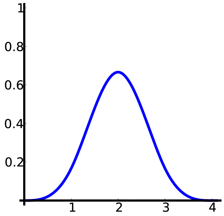
B_{X}(u):=\frac{1}{\sqrt{\det(XX^{T})}}\mathop{\mathrm{vol}}\nolimits_{N-d}\left\{(\lambda_{1},\ldots,\lambda_{N})\in[0,1]^{N}:\sum_{i=1}^{N}\lambda_{i}x_{i}=u\right\}.

For examples, see Figure 1 and Example 10. A good reference for box splines and their applications in approximation theory is [11]. Our terminology is closer to [14, Chapter 7], where splines are studied from an algebraic point of view.

A vector $u\in U$ defines a linear form $p_{x}\in\mathop{\mathrm{Sym}}\nolimits(U)$ . For a sublist $Y\subseteq X$ , we define $p_{Y}:=\prod_{y\in Y}p_{y}$ . For example, if $Y=((1,0),(1,2))$ , then $p_{Y}=s_{1}^{2}+2s_{1}s_{2}$ . Now we define the

(3)		$\displaystyle\text{\emph{central $\mathcal{P}$-space} }\mathcal{P}(X)$	$\displaystyle:=\mathop{\mathrm{span}}\{p_{Y}:\mathop{\mathrm{rk}}(X\setminus Y)=\mathop{\mathrm{rk}}(X)\}$
(4)		$\displaystyle\text{and the \emph{internal $\mathcal{P}$-space} }\mathcal{P}_{-}(X)$	$\displaystyle:=\bigcap_{x\in X}\mathcal{P}(X\setminus x).$

The space $\mathcal{P}_{-}(X)$ was introduced in [18] where it was also shown that the dimension of this space is equal to $\left|\mathcal{Z}_{-}(X)\right|$ . The space $\mathcal{P}(X)$ first appeared in approximation theory [1, 10, 16]. Later, spaces of this type and generalisations were also studied by authors in other fields, e. g. [2, 4, 19, 20, 21, 24].

We will let the elements of $\mathcal{P}_{-}(X)$ act as differential operators on the box spline. For $p\in\mathcal{P}_{-}(X)\subseteq\mathop{\mathrm{Sym}}\nolimits(U)\cong\mathbb{R}[s_{1},\ldots,s_{r}]$ , we write $p(D)$ to denote the differential operator obtained from $p$ by replacing the variable $s_{i}$ by $\frac{\partial}{\partial s_{i}}$ .

The following proposition ensures that the box spline is sufficiently smooth so that the derivatives that appear in the Main Theorem actually exist.

Proposition 1.

Let $X\subseteq\Lambda\subseteq U\cong\mathbb{R}^{d}$ be a list of vectors that is totally unimodular and let $p\in\mathcal{P}_{-}(X)$ . Then $p(D)B_{X}$ is a continuous function.

Now we are ready to state the Main Theorem. It was conjectured by Olga Holtz and Amos Ron [18, Conjecture 1.8].

Theorem 2 (Main Theorem).

Let $X\subseteq\Lambda\subseteq U\cong\mathbb{R}^{d}$ be a list of vectors that is totally unimodular. Let $f$ be a real valued function on $\mathcal{Z}_{-}(X)$ , the set of interior lattice points of the zonotope defined by $X$ .

Then there exists a unique polynomial $p\in\mathcal{P}_{-}(X)\subseteq\mathbb{R}[s_{1},\ldots,s_{d}]$ , s. t. $p(D)B_{X}$ equals $f$ on $\mathcal{Z}_{-}(X)$ .

Here, $p(D)$ denotes the differential operator obtained from $p$ by replacing the variable $s_{i}$ by $\frac{\partial}{\partial s_{i}}$ and $B_{X}$ denotes to the box spline defined by $X$ .

Remark 3.

Total unimodularity of the list $X$ is a crucial requirement in Theorem 2. Namely, the dimension of $\mathcal{P}_{-}(X)$ and $\left|\mathcal{Z}_{-}(X)\right|$ agree if and only if $X$ is totally unimodular. Note that if one vector in $X$ is multiplied by an integer $\lambda\geq 2$ , $\left|\mathcal{Z}_{-}(X)\right|$ increases while $\mathcal{P}_{-}(X)$ stays the same.

Total unimodularity also enables us to make a simple deletion-contraction proof: it implies that $\Lambda/x$ is a lattice for all $x\in X$ . In general, quotients of lattices may contain torsion elements.

Remark 4.

We have mentioned above that $\dim(\mathcal{P}_{-}(X))=\left|\mathcal{Z}_{-}(X)\right|$ holds. This is a consequence of a deep connection between the spaces $\mathcal{P}_{-}(X)$ and $\mathcal{P}(X)$ and matroid theory. The Hilbert series of these two spaces are evaluations of the Tutte polynomial of the matroid defined by $X$ [2]. One can deduce that the Hilbert series of the internal space is equal to the $h$ -polynomial of the broken-circuit complex [5] of the matroid $M^{*}(X)$ that is dual to the matroid defined by $X$ and the Hilbert series of the central space equals the $h$ -polynomial of the matroid complex of $M^{*}(X)$ . The Ehrhart polynomial of a zonotope that is defined by a totally unimodular matrix is also an evaluation of the Tutte polynomial (see e. g. [25]). In summary, for a totally unimodular matrix $X$

(5)

\dim\mathcal{P}_{-}(X)=\left|\mathcal{Z}_{-}(X)\right|={\mathfrak{T}}_{X}(0,1)\text{ and }\dim\mathcal{P}(X)=\mathop{\mathrm{vol}}(Z(X))={\mathfrak{T}}_{X}(1,1)

holds, where ${\mathfrak{T}}_{X}$ denotes the Tutte polynomial of the matroid defined by $X$ .

It is also interesting to know that the Ehrhart polynomial of an arbitrary zonotope defined by an integer matrix is an evaluation of the arithmetic Tutte polynomial [6, 7].

Figure 1. A very simple two-dimensional example. Here,

X=((1,0),(0,1),(1,1))

\mathcal{P}_{-}(X)=\mathbb{R}

, and

\left|\mathcal{Z}_{-}(X)\right|=1

Organisation of the article

In Section 2 we will discuss some basic properties of splines. We will prove the Main Theorem in the one-dimensional case in Section 3. In Section 4 we will recall the wall-crossing formula for splines and employ it to prove Proposition 1. In Section 5 we will define deletion and contraction and prove two lemmas that will be used in Section 6 in the proof of the Main Theorem.

2. Splines

In this section we will introduce the multivariate spline and discuss some basic properties of splines. Proofs of the results that we mention here can be found in [14, Chapter 7] and some also in [11].

If the convex hull of the vectors in $X$ does not contain $0$ , we define the multivariate spline (or truncated power) $T_{X}:U\to\mathbb{R}$ by

(6)

T_{X}(u):=\frac{1}{\sqrt{\det(XX^{T})}}\mathop{\mathrm{vol}}\nolimits_{N-d}\{(\lambda_{1},\ldots,\lambda_{N})\in\mathbb{R}^{N}_{\geq 0}:\sum_{i=1}^{N}\lambda_{i}x_{i}=u\}.

The support of $T_{X}$ is the cone $\mathop{\mathrm{cone}}(X):=\left\{\sum_{i=1}^{N}\lambda_{i}x_{i}:\lambda_{i}\geq 0\right\}$ .

Sometimes it is useful to think of the two splines $B_{X}$ and $T_{X}$ as distributions. In particular, one can then define the splines for lists $X\subseteq U$ that do not span $U$ .

Remark 5.

Let $X\subseteq U\cong\mathbb{R}^{r}$ be a finite list of vectors. The multivariate spline $T_{X}$ and the box spline $B_{X}$ are distributions that are characterised by the formulae

(7)		$\displaystyle\int_{U}\varphi(u)B_{X}(u)\,\mathrm{d}u$	$\displaystyle=\int_{0}^{1}\cdots\int_{0}^{1}\varphi\left(\sum_{i=1}^{N}\lambda_{i}x_{i}\right)\mathrm{d}\lambda_{1}\cdots\mathrm{d}\lambda_{N}$
(8)		$\displaystyle\text{and }\int_{U}\varphi(u)T_{X}(u)\,\mathrm{d}u$	$\displaystyle=\int_{0}^{\infty}\cdots\int_{0}^{\infty}\varphi\left(\sum_{i=1}^{N}\lambda_{i}x_{i}\right)\mathrm{d}\lambda_{1}\cdots\mathrm{d}\lambda_{N}.$

where $\varphi$ denotes a test function.

Remark 6.

Convolutions of splines are again splines. In particular,

(9)

T_{X}=T_{x_{1}}*\cdots*T_{x_{N}}\text{ and }B_{X}=B_{x_{1}}*\cdots*B_{x_{n}}.

For $x\in X$ , differentiation of the two splines in direction $x$ is particularly easy:

(10)		$\displaystyle D_{x}T_{X}$	$\displaystyle=T_{X\setminus x}$
(11)		$\displaystyle\text{ and }D_{x}B_{X}$	$\displaystyle=\nabla_{x}B_{X\setminus x}:=B_{X\setminus x}-B_{X\setminus x}(\cdot-x).$

Remark 7.

For a basis $C\subseteq U$ ,

(12)

B_{C}=\frac{\chi_{Z(C)}}{\left|\det(C)\right|}\text{ and }T_{C}=\frac{\chi_{\mathop{\mathrm{cone}}(C)}}{\left|\det(C)\right|},

where $\chi_{A}:U\to\{0,1\}$ denotes the indicator function of the set $A\subseteq U$ . In conjunction with (9), (12) provides a simple recursive method to calculate the splines.

Remark 8.

The box spline can easily be obtained from the multivariate spline. Namely,

(13)

B_{X}(u)=\sum_{S\subseteq X}(-1)^{\left|S\right|}T_{X}\left(u-a_{S}\right),

where $a_{S}:=\sum_{a\in S}a$ .

3. Cardinal $B$ -splines

In this section we will prove Theorem 2 in the one-dimensional case. This will be the base case for the inductive proof of the Main Theorem in Section 6.

Let $X_{N}:=(\underbrace{1,\ldots,1}_{N\text{ times}})\subseteq\mathbb{Z}\subseteq\mathbb{R}^{1}$ . WLOG every totally unimodular list of vectors in $\mathbb{R}^{1}$ can be written in this way.

One can easily calculate the corresponding box splines (cf. Remark 7):

(14)

B_{X_{N+1}}(u)=\int_{0}^{1}B_{X_{N}}(u-\tau)\,\mathrm{d}\tau=\sum_{j=0}^{N+1}\frac{(-1)^{j}}{N!}\binom{N+1}{j}(u-j)_{+}^{N},

where $(u-j)_{+}^{N}:=\max(u-j,0)^{N}$ . The functions $B_{X_{N+1}}$ are called cardinal $B$ -splines in the literature (e. g. [9]).

Note that $\mathcal{Z}_{-}(X_{N+1})=\{1,2,\ldots,N\}$ ,

\mathcal{P}_{X_{N+1}}=\mathop{\mathrm{span}}\{1,s,\ldots,s^{N}\},\text{ and }\mathcal{P}_{-}(X_{N+1})=\mathop{\mathrm{span}}\{1,s,\ldots,s^{N-1}\}.

Hence, in the one-dimensional case, Theorem 2 is equivalent to the following proposition.

Proposition 9.

Let $N\in\mathbb{N}$ . For every function $f:\{1,\ldots,N\}\to\mathbb{R}$ , there exist uniquely determined numbers $\lambda_{1},\ldots,\lambda_{N}\in\mathbb{R}$ s. t.

(15)

\sum_{i=1}^{N}\lambda_{i}D_{x}^{i-1}B_{X_{N+1}}(j)=f(j)\text{ for }j=1,\ldots,N.

Before proving this proposition, we give a few simple examples (see also Figure 2).

Example 10.

(16)	$\displaystyle B_{X_{2}}(s)$	$\displaystyle=s-2(s-1)_{+}+(s-2)_{+}$
(17)	$\displaystyle B_{X_{3}}(s)$	$\displaystyle=\frac{1}{2}\left({s^{2}}-3(s-1)^{2}_{+}+3(s-2)^{2}_{+}-(s-3)^{2}_{+}\right)$
(18)	$\displaystyle B_{X_{4}}(s)$	$\displaystyle=\frac{1}{6}\left({s^{3}}-4(s-1)^{3}_{+}+6(s-2)_{+}-4(s-3)^{3}_{+}+(s-4)^{3}_{+}\right)$





Figure 2. The cardinal  $B$ -splines  $B_{2}$ ,  $B_{3}$ , and  $B_{4}$ .
The matrices  $M^{N}$  are defined in (19) below.





 $\displaystyle M^{2}$ 
 $\displaystyle=\begin{pmatrix}1\end{pmatrix}\qquad\qquad M^{3}=\begin{pmatrix}\frac{1}{2}&\frac{1}{2}\\[2.84526pt] 1&-1\end{pmatrix}\qquad\qquad M^{4}=\begin{pmatrix}\frac{1}{6}&\frac{4}{6}&\frac{1}{6}\\[2.84526pt] \frac{1}{2}&0&-\frac{1}{2}\\ 1&-2&1\end{pmatrix}$ 




Proof of Proposition 9.

For  $N\in\mathbb{N}$ , we consider the matrix  $(N\times N)$ -matrix  $M^{N}$  whose entries are given by



(19)

 $m_{ij}^{N}=D_{x}^{i-1}B_{X_{N+1}}(j).$ 


The proposition is equivalent to  $M^{N}$  having full rank.
The matrix  $M^{2}=(1)$  obviously has full rank. Let us proceed by induction.
By (11),  $D_{x}^{i}B_{X_{N+1}}=\nabla_{x}D_{x}^{i-1}B_{X_{N}}$ . Thus,
the matrices satisfy the following recursion:



(20)

 $m_{ij}^{N}=m_{i-1,j}^{N-1}-m_{i-1,j-1}^{N-1}\text{ for }i=1,\ldots,N-1,\>j=1,\ldots,N,\text{ and }N\geq 2.$ 


To simplify notation, we set  $m_{i0}^{N-1}=m^{N-1}_{i,N}=0$ .
Let  $v_{k},\ldots,v_{N}$  denote the columns of  $M^{N}$ . By induction, they are linearly independent.
The columns of  $M^{N+1}$  are  $(\alpha_{1},v_{1}-v_{0}),\ldots,(\alpha_{N}+1,v_{N+1}-v_{N})$  with
 $\alpha_{j}:=B_{X_{N+1}}(j)$ . We will now show that these vectors are linearly independent as well.
Let  $\lambda_{1}\ldots,\lambda_{N+1}\in\mathbb{R}$  s. t.



(21)

 $\sum_{j=1}^{N+1}\lambda_{j}\alpha_{j}=0$ 


and
 $\lambda_{1}(v_{1}-v_{0})+\lambda_{2}(v_{2}-v_{1})+\ldots+\lambda_{N}(v_{N}-v_{N-1})-\lambda_{N+1}v_{N}=0$ .
The latter equation implies that
all  $\lambda_{i}$  are equal. We conclude that they must all be zero because of (21) and the fact that
the  $\alpha_{j}$  are positive.
∎




4. Smoothness and wall-crossing


The goal of this section is to prove Proposition 1.
Before doing this,
we mention some results on the structure of the multivariate spline  $T_{X}$  that are used in the proof. The Wall-Crossing Theorem describes
the behaviour of  $T_{X}$  when we pass from one region of polynomiality to another.


Definition 11.

A tope is a connected component of the complement of



(22)

 $\mathcal{H}_{X}:=\{\mathop{\mathrm{span}}(Y):Y\subseteq X,\,\mathop{\mathrm{rk}}(Y)=\mathop{\mathrm{rk}}(X)-1\}\subseteq U$ 





The following theorem is a consequence of Lemma 3.3 and Proposition 3.7 in [15].


Theorem 12.

Let  $X\subseteq U\cong\mathbb{R}^{d}$  be a list of vectors  $N$  that spans  $U$ 
and whose convex hull does not contain  $0$ .


Then  $T_{X}$  agrees with a homogeneous polynomial  $f^{\tau}$  of degree  $N-d$ 
on every tope  $\tau$ .



Given a hyperplane  $H$  and a tope  $\tau$  which does not intersect  $H$  (but its closure may do so),
we partition  $X\setminus H$  into two sets  $A_{H}^{\tau}$  and  $B_{H}^{\tau}$ . The set  $A_{H}^{\tau}$  contains the vectors that lie on the same side of
 $H$  as  $\tau$  and  $B_{H}^{\tau}$  contains the vectors that lie on the other side.
Note that the convex hull of  $(A_{H}^{\tau},-B_{H}^{\tau})$  does not contain  $0$ .
Hence, we can define the multivariate spline



(23)

 $T^{\tau}_{X\setminus H}:=(-1)^{\left|B_{H}^{\tau}\right|}T_{(A_{H}^{\tau},-B_{H}^{\tau})}.$ 


Now we are ready to state the wall-crossing formula as in [15, Theorem 4.10].
Related results are in [8, 22].


Theorem 13 (Wall-crossing for multivariate splines).

Let  $\tau_{1}$  and  $\tau_{2}$  be two topes whose closures have an  $r-1$  dimensional intersection  $\tau_{12}$  that spans a
hyperplane  $H$ . Then
there exists a uniquely determined distribution  $f^{\tau_{12}}$  that is supported on  $H$ 
s. t. the difference of the local pieces of  $T_{X}$  in  $\tau_{1}$  and  $\tau_{2}$  is equal to the polynomial



(24)

 $T_{X}^{\tau_{1}}-T_{X}^{\tau_{2}}=(T_{X\setminus H}^{\tau_{1}}-T_{X\setminus H}^{-\tau_{1}})*f^{\tau_{12}}.$ 





Proof of Proposition 1.

We will show that  $p(D)T_{X}$  is continuous. By (13), this implies that
 $p(D)B_{X}$  is continuous.
We may always assume that  $0$  is not contained in the convex hull of  $X$ : deleting zeroes from  $X$  changes neither  $B_{X}$  nor  $Z(X)$ .
In addition, one can always multiply a few vectors in  $X$  by  $-1$  s. t. all vectors lie on one side of some hyperplane.
This is equivalent to a translation of both,  $Z(X)$  and  $B_{X}$ .


Let  $u\in U$ . If  $u\in U\setminus\mathcal{H}_{X}$ , there is nothing to prove:
by Theorem 12,  $T_{X}$  is polynomial in a neighbourhood of  $u$  and hence smooth.
If  $u\in\mathcal{H}_{X}$ ,  $u$  is contained in the closure of at least two topes. We have to show that
the derivatives of the polynomial pieces in the topes agree on  $u$ .
This can be done using the wall-crossing formula.


It is sufficient to prove that for two topes  $\tau_{1}$  and  $\tau_{2}$  that have an  $(r-1)$ -dimensional intersection  $\tau_{12}$ ,
 $p(D)(T_{X}^{\tau_{1}}-T_{X}^{\tau_{2}})$  vanishes on  $\tau_{12}$ .


Fix a vector  $x\in X\setminus H$ . By definition,  $\mathcal{P}_{-}(X)\subseteq\mathcal{P}(X\setminus x)$ . This implies that
 $p$  can be written as a linear combination of polynomials  $p_{Y}$  where  $Y\subseteq X\setminus x$  and
 $X\setminus(Y\cup x)$  has rank  $d$ . Hence,  $X\setminus(H\cup Y)$  contains at least two vectors.


By Theorem 13,



(25)

 $\displaystyle D_{Y}(T_{X\setminus H}^{\tau_{1}}-T_{X\setminus H}^{-\tau_{1}})*f^{\tau_{12}}=(T_{X\setminus(H\cup Y)}^{\tau_{1}}-T_{X\setminus(H\cup Y)}^{-\tau_{1}})*D_{Y\cap H}f^{\tau_{12}}.$ 


This polynomial is the convolution of a distribution supported on  $H$ 
with the distribution
 $(T_{X\setminus(H\cup Y)}^{\tau_{1}}-T_{X\setminus(H\cup Y)}^{-\tau_{1}})$ . Since  $X\setminus(H\cup Y)$  contains at least
two elements, this polynomial vanishes on  $H$ . This finishes our proof.
∎



Remark 14.

Holtz and Ron conjectured that  $\mathcal{P}_{-}(X)$  is spanned by polynomials  $p_{Y}$  where  $Y$  runs
over all sublists of  $X$  s. t.  $X\setminus(Y\cup x)$  has full rank for all  $x\in X$ 
[18, Conjecture 6.1].
By formula (11), this would have implied Proposition 1.
However, this conjecture has recently been disproved [3].



5. Deletion and contraction


In this section we will introduce the operations deletion and contraction which will be used in the proof
of Theorem 2 in the next section. We will also prove two lemmas
about deletion and contraction for box splines and zonotopes.


Let  $x\in X$ . We call the list  $X\setminus x$  the deletion of  $x$ .
The image of  $X\setminus x$  under the canonical projection  $\pi_{x}:U\to U/\mathop{\mathrm{span}}(x)=:U/x$ 
is called the contraction of  $x$ . It is denoted by  $X/x$ .


The projection  $\pi_{x}$  induces a map  $\mathop{\mathrm{Sym}}\nolimits(\pi_{x}):\mathop{\mathrm{Sym}}\nolimits(U)\to\mathop{\mathrm{Sym}}\nolimits(U/x)$ .
If we identify  $\mathop{\mathrm{Sym}}\nolimits(U)$  with the polynomial ring  $\mathbb{R}[s_{1},\ldots,s_{r}]$ 
and  $x=s_{r}$ , then
 $\mathop{\mathrm{Sym}}\nolimits(\pi_{x})$  is the map from
 $\mathbb{R}[s_{1},\ldots,s_{r}]$  to  $\mathbb{R}[s_{1},\ldots,s_{r-1}]$  that sends  $s_{r}$  to zero and  $s_{1},\ldots,s_{r-1}$  to themselves.
The space  $\mathcal{P}(X/x)$  is contained in the symmetric algebra  $\mathop{\mathrm{Sym}}\nolimits(U/x)$ .


Since  $X$  is totally unimodular,  $\Lambda/x\subseteq U/x$  is a lattice for every  $x\in X$  and  $X/x$  is totally unimodular
with respect to this lattice.


Lemma 15.

Let  $x\in X$ ,  $u\in U$ , and  $\bar{u}=u+\mathop{\mathrm{span}}(x)$  the coset of  $u$  in  $X/x$ . Then



(26)

 $B_{X/x}(\bar{u})=\int_{\mathbb{R}}B_{X\setminus x}(u+\tau x)\,\mathrm{d}\tau=\sum_{\lambda\in\mathbb{Z}}B_{X}(u+\lambda x).$ 





Proof.

Let  $\bar{\varphi}:U/x\to\mathbb{R}$  be a test function and let  $\psi:U\to\mathbb{R}$  be a test function s. t.  $\bar{\varphi}(\bar{u})=\int_{\mathbb{R}}\psi(u+\tau x)\,\mathrm{d}\tau$ .
Note that a
distribution  $T$  on  $U$  that is constant on all cosets of  $\mathop{\mathrm{span}}(x)$  can be identified with a distribution  $\bar{T}$  on  $U/x$ 
via  $\bar{T}(\bar{\varphi})=T(\psi)$ . This is how (26) can be understood as an equality of distributions.
We may assume that  $x=x_{N}$ . Then



(27)

 $\displaystyle\int_{U/x}\bar{\varphi}(\bar{u})B_{X/x}(\bar{u})\,\mathrm{d}\bar{u}$ 
 $\displaystyle=\int_{0}^{1}\cdots\int_{0}^{1}\bar{\varphi}(\sum_{i}\lambda_{i}\bar{x}_{i})\,\mathrm{d}\lambda_{1}\cdots\,\mathrm{d}\lambda_{N-1}$ 


(28)


 $\displaystyle=\int_{0}^{1}\cdots\int_{0}^{1}\int_{\mathbb{R}}\psi(\sum_{i}\lambda_{i}x_{i}+\tau x)\,\mathrm{d}\tau\,\mathrm{d}\lambda_{1}\cdots\,\mathrm{d}\lambda_{N-1}$ 


(29)


 $\displaystyle=\int_{U}\psi(u){\int_{\mathbb{R}}B_{X\setminus x}(u+\tau x)}\,\mathrm{d}\tau\,\mathrm{d}u.$ 


This proves the first equality.
For the second equality, note that




 $\int_{\mathbb{R}}B_{X\setminus x}(u+\tau x)\,\mathrm{d}\tau=\sum_{\lambda\in\mathbb{Z}}\int_{0}^{1}B_{X\setminus x}(u+\lambda x-\tau x)\,\mathrm{d}\tau=\sum_{\lambda\in\mathbb{Z}}B_{X}(u+\lambda x).\qed$ 





Remark 16.

Lemma 15 is a
statement on semi-discrete and continuous convolutions with the box spline.
A related result is in [23].



The following lemma yields a deletion-contraction formula for the interior points of the zonotope.
See Figure 3
for an illustration.


Lemma 17.

The following map is a bijection:



(30)

 $\displaystyle\mathcal{Z}_{-}(X)\setminus\mathcal{Z}_{-}(X\setminus x)$ 
 $\displaystyle\to\mathcal{Z}_{-}(X/x)$ 


(31)

 $\displaystyle z$ 
 $\displaystyle\mapsto\bar{z}.$ 





Proof.

It is obvious that  $\bar{z}$  is contained in  $\mathcal{Z}_{-}(X/x)$ .
Using the fact that  $\left|\mathcal{Z}_{-}(X)\right|$  is an evaluation of the Tutte polynomial
(formula (5)) and the deletion-contraction formula for the
Tutte polynomial, one can easily establish that the domain and the range of the map have the same cardinality.


Hence it is sufficient to show that the map is injective.
Let us prove this. First note that  $z\in\mathcal{Z}_{-}(X)$  is contained  $\mathcal{Z}_{-}(X\setminus x)$  if and only if
 $z+x\in\mathcal{Z}_{-}(X)$ .
Let  $z_{1},z_{2}\in\mathcal{Z}_{-}(X)\setminus\mathcal{Z}_{-}(X\setminus x)$  s. t.  $\bar{z}_{1}=\bar{z}_{2}$ . This implies that there is
a  $\lambda\in\mathbb{R}$  s. t.  $z_{1}=z_{2}+\lambda x$ . Because of the total unimodularity,  $\lambda$  must be
an integer. WLOG  $\lambda$  is non-negative.
By convexity,  $z_{1},\ldots,z_{1}+x,\ldots,z_{1}+\lambda x$  are contained in  $\mathcal{Z}_{-}(X)$ .
By the observation at the beginning of this paragraph,  $z_{1}+x$  is not
contained in  $\mathcal{Z}_{-}(X)$ . This implies  $\lambda=0$ . Hence the map is injective.
∎



6. Exact sequences


In this section we will prove the Main Theorem.
We start with a simple observation.


Remark 18.

If  $X$  contains a coloop, i. e. an element  $x$  s. t.  $\mathop{\mathrm{rk}}(X\setminus x)<\mathop{\mathrm{rk}}(X)$ , then
 $\mathcal{Z}_{-}(X)=\emptyset$ 
and  $\mathcal{P}_{-}(X)=\{0\}$ . Hence,
Theorem 2 is trivially satisfied.



We will consider the set
 $\Xi(X):=\{f:\Lambda\to\mathbb{R}:\mathop{\mathrm{supp}}\nolimits(f)\subseteq\mathcal{Z}_{-}(X)\}$ 
and the map



(32)

 $\displaystyle\begin{split}\gamma_{X}:\mathcal{P}_{-}(X)&\to\Xi(X)\\ p&\mapsto\bigl[\>\Lambda\ni z\mapsto p(D)B_{X}(z)\>\bigr]\end{split}$ 




Figure 3. Deletion and contraction for a zonotope and a function defined on the interior lattice points of
the zonotope.



Proposition 19.

Let  $d\geq 2$  and let  $\Lambda\subseteq U\cong\mathbb{R}^{d}$  be a lattice.
Let  $X\subseteq\Lambda$  be a finite list of vectors that spans  $U$ 
and that is totally unimodular with respect to  $\Lambda$ .
Let  $x\in X$  be a non-zero element s. t.  $\mathop{\mathrm{rk}}(X\setminus x)=\mathop{\mathrm{rk}}(X)$ .


Then
the following diagram of real vector spaces is
commutative, the rows are exact and the vertical maps are isomorphisms:










(37)

 $\displaystyle\text{where }\nabla_{x}(f)(z)$ 
 $\displaystyle:=f(z)-f(z-x),$ 


(38)

 $\displaystyle\Sigma_{x}(f)(\bar{z})$ 
 $\displaystyle:=\sum_{x\in\bar{z}\cap\Lambda}f(x)=\sum_{\lambda\in\mathbb{Z}}f(\lambda x+z)\text{ for some }z\in\bar{z}.$ 





Proof.

Commutativity of the left square:
Let  $z\in\mathcal{Z}_{-}(X)$  and let  $p\in\mathcal{P}_{-}(X\setminus x)$ .
By (11),
 $(p\cdot p_{x})(D)B_{X}(z)=\nabla_{x}(p(D)B_{X\setminus x})(z)$ .
Hence  $\gamma_{X}\circ(\cdot p_{x})=\nabla_{x}\circ\gamma_{X\setminus x}$ .


Commutativity of the right square:
Let  $\bar{z}\in\mathcal{Z}_{-}(X/x)$ ,  $f\in\mathcal{P}_{-}(X)$  and let  $z\in U$  be a representative of  $\bar{z}$ .
Then




 $\sum_{\lambda\in\mathbb{Z}}p(D)B_{X}(\lambda x+z)=p(D)\int_{\mathbb{R}}B_{X\setminus x}(u+\tau x)\,\mathrm{d}\tau=\mathop{\mathrm{Sym}}\nolimits(\pi_{x})(p)(D)B_{X/x}(\bar{z})$ 


because of Lemma 15 and the fact that
applying a differential operator to a function that is constant on a subspace is the same
as applying the projection of the differential operator to
the projection of the function.
Hence  $\gamma_{X/x}\circ\mathop{\mathrm{Sym}}\nolimits(\pi_{x})=\Sigma_{x}\circ\gamma_{X}$ .


Exactness:
Exactness of the first row was stated in [2] and proven in [20].
The proof relies on the fact that  $\mathcal{P}_{-}(X)$  can be written as the kernel of a power ideal.
Exactness of the second row is easy to check
taking into account
Lemma 17.


Isomorphisms:
By induction over the number of non-zero elements in  $X$ ,  $\gamma_{X\setminus x}$  and  $\gamma_{X/x}$  are isomorphisms.
Then  $\gamma_{X}$  is also an isomorphism by the five lemma.


Two base cases have to be considered: by deleting elements from  $X$ , it may happen that  $X$  eventually contains only coloops and zeroes.
This case is trivial (cf. Remark 18).


By contracting elements from  $X$ , it may happen that  $X$  has rank  $1$ . We have shown in
Section 3 that
 $\mathcal{P}_{-}(X)$  and  $\Xi(X)$  are isomorphic in this case.
∎



Proof of the Main Theorem.

The theorem is equivalent
to  $\gamma_{X}$  being an isomorphism, which is part of
Proposition 19.
∎



References


                    
[1]

A. A. Akopyan and A. A. Saakyan, A system of differential equations that
is related to the polynomial class of translates of a box spline, Mat.
Zametki 44 (1988), no. 6, 705–724, 861. 


                    
[2]

Federico Ardila and Alexander Postnikov, Combinatorics and geometry of
power ideals, Trans. Amer. Math. Soc. 362 (2010), no. 8,
4357–4384. 


                    
[3]

by same author, Two counterexamples for power ideals of hyperplane
arrangements, 2012, personal communication, to appear as a corrigendum for
[2].


                    
[4]

Andrew Berget, Products of linear forms and Tutte polynomials,
European J. Combin. 31 (2010), no. 7, 1924–1935. 


                    
[5]

Tom Brylawski, The broken-circuit complex, Trans. Amer. Math. Soc.
234 (1977), no. 2, 417–433. 


                    
[6]

Michele D’Adderio and Luca Moci, Ehrhart polynomial and arithmetic
Tutte polynomial, European J. Combin. 33 (2012), no. 7, 1479 –
1483.


                    
[7]

Michele D’Adderio and Luca Moci, Arithmetic matroids, the Tutte
polynomial and toric arrangements, Advances in Mathematics 232
(2013), no. 1, 335–367.


                    
[8]

Wolfgang Dahmen and Charles A. Micchelli, The number of solutions to
linear Diophantine equations and multivariate splines, Trans. Amer. Math.
Soc. 308 (1988), no. 2, 509–532. 


                    
[9]

Carl de Boor, Splines as linear combinations of  $B$ -splines. A
survey, Approximation theory, II (Proc. Internat. Sympos., Univ.
Texas, Austin, Tex., 1976), Academic Press, New York, 1976, pp. 1–47.



                    
[10]

Carl de Boor, Nira Dyn, and Amos Ron, On two polynomial spaces associated
with a box spline, Pacific J. Math. 147 (1991), no. 2, 249–267.



                    
[11]

Carl de Boor, Klaus Höllig, and Sherman D. Riemenschneider, Box
splines, Applied Mathematical Sciences, vol. 98, Springer-Verlag, New York,
1993. 


                    
[12]

Carl de Boor and Amos Ron, On multivariate polynomial interpolation.,
Constructive Approximation 6 (1990), no. 3, 287–302 (English).


                    
[13]

by same author, The least solution for the polynomial interpolation problem,
Math. Z. 210 (1992), no. 3, 347–378. 


                    
[14]

Corrado De Concini and Claudio Procesi, Topics in hyperplane
arrangements, polytopes and box-splines, Universitext, Springer, New York,
2011. 


                    
[15]

Corrado De Concini, Claudio Procesi, and Michèle Vergne, Vector
partition functions and generalized Dahmen and Micchelli spaces,
Transform. Groups 15 (2010), no. 4, 751–773. 


                    
[16]

Nira Dyn and Amos Ron, Local approximation by certain spaces of
exponential polynomials, approximation order of exponential box splines, and
related interpolation problems, Trans. Amer. Math. Soc. 319 (1990),
no. 1, 381–403. 


                    
[17]

Mariano Gasca and Thomas Sauer, Polynomial interpolation in several
variables, Adv. Comput. Math. 12 (2000), no. 4, 377–410,
Multivariate polynomial interpolation. 


                    
[18]

Olga Holtz and Amos Ron, Zonotopal algebra, Advances in Mathematics
227 (2011), no. 2, 847–894. 


                    
[19]

Olga Holtz, Amos Ron, and Zhiqiang Xu, Hierarchical zonotopal spaces,
Trans. Amer. Math. Soc. 364 (2012), 745–766. 


                    
[20]

Matthias Lenz, Hierarchical zonotopal power ideals, European J. Combin.
33 (2012), no. 6, 1120–1141.


                    
[21]

by same author, Zonotopal algebra and forward exchange matroids, 2012,
arXiv:1204.3869v2.


                    
[22]

András Szenes and Michèle Vergne, Residue formulae for vector
partitions and Euler-MacLaurin sums, Adv. in Appl. Math. 30
(2003), no. 1-2, 295–342, Formal power series and algebraic combinatorics
(Scottsdale, AZ, 2001). 


                    
[23]

Michèle Vergne, A remark on the convolution with the box spline,
Ann. of Math. (2) 174 (2011), no. 1, 607–618. 


                    
[24]

David G. Wagner, Algebras related to matroids represented in
characteristic zero, European J. Combin. 20 (1999), no. 7,
701–711. 


                    
[25]

Dominic Welsh, The Tutte polynomial, Random Structures Algorithms
15 (1999), no. 3-4, 210–228, Statistical physics methods in
discrete probability, combinatorics, and theoretical computer science
(Princeton, NJ, 1997).

(27)	$\displaystyle\int_{U/x}\bar{\varphi}(\bar{u})B_{X/x}(\bar{u})\,\mathrm{d}\bar{u}$	$\displaystyle=\int_{0}^{1}\cdots\int_{0}^{1}\bar{\varphi}(\sum_{i}\lambda_{i}\bar{x}_{i})\,\mathrm{d}\lambda_{1}\cdots\,\mathrm{d}\lambda_{N-1}$
(28)		$\displaystyle=\int_{0}^{1}\cdots\int_{0}^{1}\int_{\mathbb{R}}\psi(\sum_{i}\lambda_{i}x_{i}+\tau x)\,\mathrm{d}\tau\,\mathrm{d}\lambda_{1}\cdots\,\mathrm{d}\lambda_{N-1}$
(29)		$\displaystyle=\int_{U}\psi(u){\int_{\mathbb{R}}B_{X\setminus x}(u+\tau x)}\,\mathrm{d}\tau\,\mathrm{d}u.$

(30)		$\displaystyle\mathcal{Z}_{-}(X)\setminus\mathcal{Z}_{-}(X\setminus x)$	$\displaystyle\to\mathcal{Z}_{-}(X/x)$
(31)		$\displaystyle z$	$\displaystyle\mapsto\bar{z}.$

(37)		$\displaystyle\text{where }\nabla_{x}(f)(z)$	$\displaystyle:=f(z)-f(z-x),$
(38)		$\displaystyle\Sigma_{x}(f)(\bar{z})$	$\displaystyle:=\sum_{x\in\bar{z}\cap\Lambda}f(x)=\sum_{\lambda\in\mathbb{Z}}f(\lambda x+z)\text{ for some }z\in\bar{z}.$

Interpolation, box splines, and lattice points in zonotopes Thanks: The author was supported by an ERC starting grant awarded to Olga Holtz and subsequently by a Junior Research Fellowship of Merton College (University of Oxford).

Abstract.

Key words and phrases:

2010 Mathematics Subject Classification

1. Introduction

Proposition 1.

Theorem 2 (Main Theorem).

Remark 3.

Remark 4.

Organisation of the article

2. Splines

Remark 5.

Remark 6.

Remark 7.

Remark 8.

3. Cardinal BB-splines

Proposition 9.

Example 10.

Proof of Proposition 9.

4. Smoothness and wall-crossing

Definition 11.

Theorem 12.

Theorem 13 (Wall-crossing for multivariate splines).

Proof of Proposition 1.

Remark 14.

5. Deletion and contraction

Lemma 15.

Proof.

Remark 16.

Lemma 17.

Proof.

6. Exact sequences

Remark 18.

Proposition 19.

Proof.

Proof of the Main Theorem.

References

3. Cardinal $B$ -splines