跳到论文正文
W Papers独立论文阅读器 arXiv:1211.1098 论文正文 计算阅读时间 · 0%
引用这篇论文根据当前论文元数据生成,正式投稿前建议核对。


License: arXiv.org perpetual non-exclusive license
arXiv:1211.1098v3 [quant-ph] 09 Feb 2014

Disguising quantum channels by mixing and channel distance trade-off

Chi-Hang Fred Fung    H. F. Chau Affiliation: Department of Physics and Center of Theoretical and Computational Physics, University of Hong Kong, Pokfulam Road, Hong Kong Email: chffung@hku.hk
Abstract

We consider the reverse problem to the distinguishability of two quantum channels, which we call the disguising problem. Given two quantum channels, the goal here is to make the two channels identical by mixing with some other channels with minimal mixing probabilities. This quantifies how much one channel can disguise as the other. In addition, the possibility to trade off between the two mixing probabilities allows one channel to be more preserved (less mixed) at the expense of the other. We derive lower- and upper-bounds of the trade-off curve and apply them to a few example channels. Optimal trade-off is obtained in one example. We relate the disguising problem and the distinguishability problem by showing the the former can lower and upper bound the diamond norm. We also show that the disguising problem gives an upper bound on the key generation rate in quantum cryptography.

pacs
03.67.Hk, 03.67.Lx, 03.67.Dd

1 Introduction

Quantum information processing involves the transformation of quantum states through quantum channels and it is often useful to quantify how far apart quantum states or quantum channels are. Depending on the problem at hand, different ways of measuring the distance may be adopted. Trace distance [1, 2] and fidelity [3, 4, 5] are two widely-used measures for quantum states. Trace distance is particularly interesting because it corresponds to a measurement that distinguishes between two quantum states with the minimum error. Other distances for quantum states have also been studied recently, including the Monge distance [6], the kkth operator norm [7], and the partitioned trace distance [8]. For quantum channels, measures [9] have also been proposed based on extending the fidelity measure [10] and the trace distance measure [11] of quantum states. The diamond norm, in particular, is a trace-distance-based measure for quantum channels. It was first introduced in quantum information processing by Kitaev [11] for studying quantum error correction and has a nice operational meaning because it corresponds to minimum-error channel discrimination. As such, the diamond norm has been receiving a lot of attention since its introduction, in both the theoretical aspect [12, 13, 14, 15, 16, 17] and the computational aspect [18, 19].

While distinguishability (of quantum states and channels) is a well studied problem, we consider the reverse problem – the disguising problem for quantum channels. Unlike the distinguishability problem in which the goal is to find a measurement that distinguishes between two (or more) states or channels, the aim in the disguising problem is to find out the minimal mixing needed to make two (or more) quantum channels completely identical. In essence, this quantifies how much the effect of one channel is partially carried out by another channel. In this pilot study, we investigate the disguising problem for two channels.

As we show in this paper, the disguising problem and the distinguishability problem can be considered as dual to each other. We establish this by showing that the solution of the disguising problem can be used to lower and upper bound the diamond norm, which is a measure of distinguishability. This has an interesting implication: the more distinguishable two quantum channels are, the more effort it takes to disguise one as the other. Additionally, the disguising problem can be cast as a semidefinite program and we also show efficient ways to compute lower- and upper-bounds of it. We note that the diamond norm can be computed using semidefinite/convex programming and Monte Carlo methods [20, 18, 21, 19].

The disguising problem can be understood with the following operational interpretation. First note that the operational meaning of the diamond norm is based on the perspective of the receiver who tries to distinguish between two channels. A reverse perspective is to look at the channel intervener who tries to make the channels identical by minimal intervention. The channel intervener possesses the two original channels as black boxes. She is not allowed to open them and is only allowed to occasionally substitute each of them with some other arbitrary channel. We ask what are the minimal mixing probabilities needed to make the two intervened channels identical?

The precise problem statement is the following. Given two quantum channels ℰ⁡(ρ)=∑iEi​ρ​Ei†\mathcal{E}(\rho)=\sum_{i}E_{i}\rho E_{i}^{\dagger} and ℱ⁡(ρ)=∑iFi​ρ​Fi†\mathcal{F}(\rho)=\sum_{i}F_{i}\rho F_{i}^{\dagger} acting on an nn-dimensional Hilbert space where EiE_{i} and FiF_{i} are n×nn\times n complex matrices representing the Kraus operators of the channels, we consider the processing

ℰ​(ρ)→ℰ′​(ρ)\displaystyle\mathcal{E}(\rho)\rightarrow\mathcal{E}^{\prime}(\rho) =\displaystyle= (1−p)​ℰ​(ρ)+p​ℰΔ​(ρ),\displaystyle(1-p)\mathcal{E}(\rho)+p\mathcal{E}_{\Delta}(\rho), (1)
ℱ​(ρ)→ℱ′​(ρ)\displaystyle\mathcal{F}(\rho)\rightarrow\mathcal{F}^{\prime}(\rho) =\displaystyle= (1−q)​ℱ​(ρ)+q​ℱΔ​(ρ)\displaystyle(1-q)\mathcal{F}(\rho)+q\mathcal{F}_{\Delta}(\rho) (2)

such that ℰ′=ℱ′\mathcal{E}^{\prime}=\mathcal{F}^{\prime} with “the smallest” pp and qq (which will be clarified later as the distance profile). In other words, we are interested in the least amount of substitution of ℰ\mathcal{E} and ℱ\mathcal{F} needed to make them equal. This is illustrated in figure 2. Operationally, the new channel probabilistically selects between the original channel and some other harmonizing channel, ℰΔ\mathcal{E}_{\Delta} or ℱΔ\mathcal{F}_{\Delta}, which is yet to be determined. The smaller the mixing probability, pp or qq, the closer the new channel is to the original one. Thus, pp and qq serve as a distance between the two channels. We note that in general the harmonizing channels ℰΔ\mathcal{E}_{\Delta} and ℱΔ\mathcal{F}_{\Delta} are not universal and depend on the original channels ℰ\mathcal{E} and ℱ\mathcal{F}. In fact, the problem becomes trivial if we insist ℰΔ\mathcal{E}_{\Delta} and ℱΔ\mathcal{F}_{\Delta} to be universal for then ℰΔ=ℱΔ\mathcal{E}_{\Delta}=\mathcal{F}_{\Delta} (with either p=q=1p=q=1 when ℰ≠ℱ\mathcal{E}\neq\mathcal{F} or p=q=0p=q=0 when ℰ=ℱ\mathcal{E}=\mathcal{F}). Also, note that ℰ′=ℱ′\mathcal{E}^{\prime}=\mathcal{F}^{\prime} is trivially satisfied with ℰΔ=ℱ\mathcal{E}_{\Delta}=\mathcal{F}, ℱΔ=ℰ\mathcal{F}_{\Delta}=\mathcal{E}, and p+q=1p+q=1. This gives a linear trade-off between pp and qq. However, in general, better sub-linear trade-off can be obtained, as we show later. Note that ℰΔ\mathcal{E}_{\Delta} and ℱΔ\mathcal{F}_{\Delta} can be general quantum channels with arbitrary complexity.

Refer to caption
Figure 1: Achievable trade-off region and distance profile of the channel disguising problem. When the mixing probabilities pp and qq are too small (corresponding to the forbidden region), the channels ℰ\mathcal{E} and ℱ\mathcal{F} cannot be made equal.

The pair of parameters (p,q)(p,q) represents the trade-off between the two channels’ mixing probabilities. The more mixing is imposed on one channel, the less mixing is required on the other. Note that if (p,q)(p,q) is a trade-off point, (p+δ​p,q+δ​q)(p+\delta p,q+\delta q) with δ​p,δ​q≥0\delta p,\delta q\geq 0 is a also a trade-off point (and we call the former point strictly better than the latter). When given a region of achievable trade-off points, a trade-off curve can be obtained by tracing out the boundary such that no point is strictly better than another. This gives us a distance profile for the two channels (see figure 1). Thus, our measure is unique in that it is represented by a 2-dimensional curve rather than a scalar as in other measures for quantum channels. On the other hand, a scalar distance may be obtained from our measure in several ways, for example, (i) by imposing equal mixing probabilities p=qp=q and regarding the minimum p=qp=q as the distance between the two channels, or (ii) by regarding the minimum p+qp+q as the distance. We will justify that these two are distances by showing that the triangle inequality holds.

Refer to caption
Figure 2: Two quantum channels, ℰ\mathcal{E} and ℱ\mathcal{F}, are made identical by mixing the original channel ℰ\mathcal{E} (ℱ\mathcal{F}) with a harmonizing channel ℰΔ\mathcal{E}_{\Delta} (ℱΔ\mathcal{F}_{\Delta}) with probability pp (qq). The designer is free to choose the non-shaded parts ℰΔ\mathcal{E}_{\Delta} and ℱΔ\mathcal{F}_{\Delta}, but not ℰ\mathcal{E} and ℱ\mathcal{F}.

The disguising problem admits a geometric interpretation. Given a channel ℰ\mathcal{E}, we denote the set of all channels achieved by mixing channel ℰ\mathcal{E} with arbitrary harmonizing channels and mixing probability pp as

Sp​(ℰ)\displaystyle S_{p}(\mathcal{E}) ≡\displaystyle\equiv {ℰ′:ℰ′=(1−p)ℰ+pℰΔ, for some harmonizing channel ℰΔ}.\displaystyle\{\mathcal{E}^{\prime}:\mathcal{E}^{\prime}=(1-p)\mathcal{E}+p\mathcal{E}_{\Delta},\text{ for some harmonizing channel }\mathcal{E}_{\Delta}\}.

Note that Sp′⊂SpS_{p^{\prime}}\subset S_{p} for p′<pp^{\prime}<p for the following reason. For any ℰ′∈Sp′\mathcal{E}^{\prime}\in S_{p^{\prime}}, we have

ℰ′\displaystyle\mathcal{E}^{\prime} =\displaystyle= (1−p′)​ℰ+p′​ℰΔ\displaystyle(1-p^{\prime})\mathcal{E}+p^{\prime}\mathcal{E}_{\Delta}
=\displaystyle= (1−p)​ℰ+[p′​ℰΔ+(p−p′)​ℰ]\displaystyle(1-p)\mathcal{E}+[p^{\prime}\mathcal{E}_{\Delta}+(p-p^{\prime})\mathcal{E}]

where the term in bracket is a valid quantum channel scaled by pp. Thus, ℰ′\mathcal{E}^{\prime} can be regarded as having mixing probability pp and so ℰ′∈Sp\mathcal{E}^{\prime}\in S_{p}. It can be easily checked that Sp​(ℰ)S_{p}(\mathcal{E}) is compact and convex. This enables a geometric interpretation of the disguising problem as a search for pp and qq so that Sp​(ℰ)S_{p}(\mathcal{E}) and Sq​(ℱ)S_{q}(\mathcal{F}) just meet (see figure 3).

Refer to caption

(a)

Refer to caption

(b)

Figure 3: Geometric interpretation of the disguising problem. The set of channels within mixing probability pp (qq) from channel ℰ\mathcal{E} (ℱ\mathcal{F}) is denoted as Sp​(ℰ)S_{p}(\mathcal{E}) (Sq​(ℱ)S_{q}(\mathcal{F})). In (a), we search for pp and qq so that the two sets meet. In (b), they meet with different parameters p′p^{\prime} and q′q^{\prime}.

In this paper, we formulate the disguising problem as an optimization problem and present our main result in section 3. Although solving it turns out to be difficult, we are able to obtain lower-bound and upper-bound on the (p,q)(p,q) trade-off curve (cf. equation (15)). In section 4, we prove the main result, which is the lower- and upper-bounds. Next, we illustrate the computation of the bounds in a few examples for different quantum channels in section 5. In one special case, the analytical lower- and upper-bounds coincide, effectively producing the optimal trade-off curve. For the other cases, the numerically computed lower- and upper-bounds are quite tight, showing the effectiveness of the bounds. In section 6, we show that the disguising problem can lower and upper bound the diamond norm which quantifies the distinguishability of two quantum channels. We also make three remarks about our distance profile for quantum channels in section 7. We discuss one application of the disguising problem in section 8, which is to bound the key generation rate in quantum cryptography. We conclude in section 9.

2 Notation

We denote a matrix AA to be positive-semidefinite (PSD) by A⪰0A\succeq 0, the transpose of AA by AtA^{t}, and the conjugate transpose of AA by A†A^{\dagger}. AA is PSD if and only if AA is Hermitian and its eigenvalues are non-negative. \lVert​A​\rVert\lVert A\rVert denotes the spectral norm of AA which is the largest singular value of AA or the largest eigenvalue of AA if AA is PSD. \lVert​A​\rVert1≜Tr​A†​A\lVert A\rVert_{1}\triangleq{\rm Tr}\sqrt{A^{\dagger}A} denotes the trace norm of AA.

ℬ⁡(ℋn)\mathcal{B}(\mathcal{H}_{n}) denotes the set of all bounded linear operators in an nn-dimensional Hilbert space ℋn\mathcal{H}_{n}. IpI_{p} denotes the identity operator in a pp-dimensional Hilbert space. A linear map ℰ:ℬ⁡(ℋn)→ℬ⁡(ℋn)\mathcal{E}:\mathcal{B}(\mathcal{H}_{n})\rightarrow\mathcal{B}(\mathcal{H}_{n}) is positive if ℰ⁡(A)\mathcal{E}(A) is PSD for all PSD AA in ℬ⁡(ℋn)\mathcal{B}(\mathcal{H}_{n}), and ℰ\mathcal{E} is completely positive (CP) if ℰ⊗Ip\mathcal{E}\otimes I_{p} is positive for all positive integers pp. ℰ\mathcal{E} is trace-preserving (TP) if Tr⁡(ℰ⁡(A))=Tr⁡(A){\rm Tr}(\mathcal{E}(A))={\rm Tr}(A) for all AA in ℬ⁡(ℋn)\mathcal{B}(\mathcal{H}_{n}).

A linear map ℰ:ℬ⁡(ℋn)→ℬ⁡(ℋn)\mathcal{E}:\mathcal{B}(\mathcal{H}_{n})\rightarrow\mathcal{B}(\mathcal{H}_{n}) can be represented by a Choi matrix of size n2×n2n^{2}\times n^{2} [22]:

Cℰ\displaystyle C_{\mathcal{E}} =\displaystyle= [ℰ⁡(|0⟩⟨0|)ℰ⁡(|0⟩⟨1|)…ℰ⁡(|0⟩⟨n−1|)ℰ⁡(|1⟩⟨0|)⋱⋮ℰ⁡(|n−1⟩⟨0|)…ℰ⁡(|n−1⟩⟨n−1|)]\displaystyle\left[\hskip-5.0pt\begin{array}[]{*\c@MaxMatrixCols c}\mathcal{E}(\mbox{$\left|0\right\rangle$}\mbox{$\left\langle 0\right|$})&\mathcal{E}(\mbox{$\left|0\right\rangle$}\mbox{$\left\langle 1\right|$})&\dots&\mathcal{E}(\mbox{$\left|0\right\rangle$}\mbox{$\left\langle n-1\right|$})\\ \mathcal{E}(\mbox{$\left|1\right\rangle$}\mbox{$\left\langle 0\right|$})&\ddots\\ \vdots\\ \mathcal{E}(\mbox{$\left|n-1\right\rangle$}\mbox{$\left\langle 0\right|$})&\dots&&\mathcal{E}(\mbox{$\left|n-1\right\rangle$}\mbox{$\left\langle n-1\right|$})\end{array}\hskip-5.0pt\right] (8)
=\displaystyle= ∑i,j=0n−1|i⟩⟨j|⊗ℰ⁡(|i⟩⟨j|).\displaystyle\sum_{i,j=0}^{n-1}\mbox{$\left|i\right\rangle$}\mbox{$\left\langle j\right|$}\otimes\mathcal{E}(\mbox{$\left|i\right\rangle$}\mbox{$\left\langle j\right|$}).

We define a function, which we call the channel sum function, of the Choi matrix CℰC_{\mathcal{E}} of a linear map ℰ\mathcal{E} as follows:

𝕋⁡(Cℰ)\displaystyle{\mathbb{T}}(C_{\mathcal{E}}) :⁣=\displaystyle:= Tr2t​(Cℰ)\displaystyle{\rm Tr}_{2}^{t}(C_{\mathcal{E}}) (9)
=\displaystyle= ∑i,j=0n−1|i⟩⟨j|⋅Tr⁡[ℰ⁡(|j⟩⟨i|)],\displaystyle\sum_{i,j=0}^{n-1}\mbox{$\left|i\right\rangle$}\mbox{$\left\langle j\right|$}\cdot{\rm Tr}[\mathcal{E}(\mbox{$\left|j\right\rangle$}\mbox{$\left\langle i\right|$})], (10)

where Tr2{\rm Tr}_{2} is the partial trace over the second system and tt represents transpose. We remark that 𝕋⁡(Cℰ)=I{\mathbb{T}}(C_{\mathcal{E}})=I if and only if ℰ\mathcal{E} is trace-preserving (see Lemma 5 in A).

3 Problem formulation and main result

3.1 Optimization problem formulation

To solve for the optimal distance profile (p,q)(p,q) of equations (1) and (2) with the condition that the new channels are identical, i.e., ℰ′=ℱ′\mathcal{E}^{\prime}=\mathcal{F}^{\prime}, we formulate the problem as (see figure 1):

minimize q\displaystyle\>q (11)
subject to ℰ′=ℱ′,\displaystyle\mathcal{E}^{\prime}=\mathcal{F}^{\prime},
CℰΔ⪰0,\displaystyle C_{\mathcal{E}_{\Delta}}\succeq 0,
CℱΔ⪰0,\displaystyle C_{\mathcal{F}_{\Delta}}\succeq 0,
𝕋⁡(CℰΔ)=I,\displaystyle{\mathbb{T}}(C_{\mathcal{E}_{\Delta}})=I,
𝕋⁡(CℱΔ)=I,\displaystyle{\mathbb{T}}(C_{\mathcal{F}_{\Delta}})=I,

where the minimization is over qq, ℰΔ\mathcal{E}_{\Delta}, and ℱΔ\mathcal{F}_{\Delta}, for some fixed pp. Here, we denote the Choi matrices of ℰΔ\mathcal{E}_{\Delta} and ℱΔ\mathcal{F}_{\Delta} by CℰΔC_{\mathcal{E}_{\Delta}} and CℱΔC_{\mathcal{F}_{\Delta}}, respectively (see equation (2)), and 𝕋{\mathbb{T}} is the channel sum function defined in equation (9). The last four constraints demand that ℰΔ\mathcal{E}_{\Delta} and ℱΔ\mathcal{F}_{\Delta} be quantum channels (TPCP maps) (cf. Theorem 3 and Lemma 5 in A). Note that the roles of pp and qq in the formulation of the above optimization problem may be interchanged (i.e., we may have “fix qq and minimize pp” instead). We remark that this problem can be cast as a semidefinite program with the use of equation (17) and may be solved numerically. However, in this paper, we are interested in the analytical bounds of this problem and the investigation of the trade-off behavior between pp and qq.

Note that for p=1p=1, the solution of q=0q=0 is trivially obtained to make ℰ′=ℱ′\mathcal{E}^{\prime}=\mathcal{F}^{\prime}, since we can choose ℰΔ=ℱ\mathcal{E}_{\Delta}=\mathcal{F} in equations (1) and (2). By the same token, (p,q)=(0,1)(p,q)=(0,1) is feasible.

The distance profile (such as that in figure 1) should be convex. This is because given two points (p,q)(p,q) and (p′,q′)(p^{\prime},q^{\prime}) that satisfy ℰ′=ℱ′\mathcal{E}^{\prime}=\mathcal{F}^{\prime} [see equations (1) and (2)], any linear combination of them [i.e., ((1−t)​p+t​p′,(1−t)​q+t​q′)((1-t)p+tp^{\prime},(1-t)q+tq^{\prime}) for some 0≤t≤10\leq t\leq 1] also satisfies it. It follows that any point on the line q=1−pq=1-p is a feasible solution.

Refer to caption
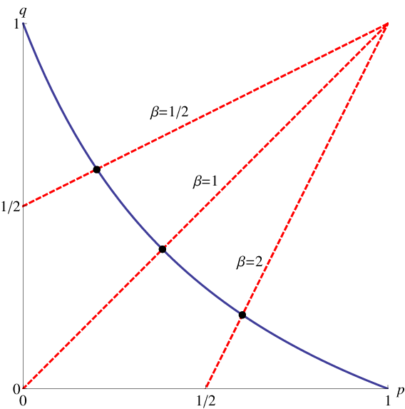
Figure 4: Distance profile obtained by solving problem (12). Among all the points (p,q)(p,q) along the line corresponding to a fixed value of β\beta, we choose the point with the minimum qq subject to the constraints of the problem. For each value of β\beta, we solve the optimization problem and obtain an optimal point (p,q)(p,q). Repeating this for a range of β\beta produces the solid curve.

3.2 Main result

Our main result is the lower- and upper-bounds of the distance profile generated by the solutions of problem (11). It turns out that it is easier to analyze and present the main result by expressing the problem as follows:

minimize q\displaystyle\>q (12)
subject to ℰ′=ℱ′,\displaystyle\mathcal{E}^{\prime}=\mathcal{F}^{\prime},
β=1−q1−p,\displaystyle\beta=\frac{1-q}{1-p},
CℰΔ⪰0,\displaystyle C_{\mathcal{E}_{\Delta}}\succeq 0,
CℱΔ⪰0,\displaystyle C_{\mathcal{F}_{\Delta}}\succeq 0,
𝕋⁡(CℰΔ)=I,\displaystyle{\mathbb{T}}(C_{\mathcal{E}_{\Delta}})=I,
𝕋⁡(CℱΔ)=I,\displaystyle{\mathbb{T}}(C_{\mathcal{F}_{\Delta}})=I,

where the minimization is over pp, qq, ℰΔ\mathcal{E}_{\Delta}, and ℱΔ\mathcal{F}_{\Delta}, for some fixed parameter β\beta. Here, β\beta is a new parameter and the distance profile (p,q)(p,q) is obtained by solving this optimization problem over a range of β\beta (see figure 4).

Our main result is that the distance profile (p,q)(p,q) is bounded from below and above as follows:

p\displaystyle p =\displaystyle= 1−1α+β, and\displaystyle 1-\frac{1}{\alpha+\beta},\text{ and} (13)
q\displaystyle q =\displaystyle= αα+β\displaystyle\frac{\alpha}{\alpha+\beta} (14)

where β\beta is fixed and

n−1​Tr​[𝕋⁡(Δ+)]≤α≤min⁡(\lVert​𝕋​(Δ+)​\rVert,1).\displaystyle n^{-1}{\rm Tr}[{\mathbb{T}}(\Delta_{+})]\leq\alpha\leq\min(\lVert{\mathbb{T}}(\Delta_{+})\rVert,1). (15)

Here, Δ+\Delta_{+} is a PSD matrix obtained by decomposing Cℰ−β​CℱC_{\mathcal{E}}-\beta C_{\mathcal{F}} into the positive and negative subspaces by eigen-decomposition:

Cℰ−β​Cℱ=Δ+−Δ−,C_{\mathcal{E}}-\beta C_{\mathcal{F}}=\Delta_{+}-\Delta_{-}, (16)

where Δ±\Delta_{\pm} are PSD matrices with support on orthogonal vector spaces (i.e., Δ+​Δ−=0\Delta_{+}\Delta_{-}=0) and CℰC_{\mathcal{E}} and CℱC_{\mathcal{F}} are the Choi matrices for the quantum channels ℰ\mathcal{E} and ℱ\mathcal{F}, respectively. Also, nn is the dimension of the quantum states on which the channels act.

Note that d​p/d​α>0dp/d\alpha>0 and d​q/d​α>0dq/d\alpha>0 implying that a smaller α\alpha gives rise to a “smaller” pair (p,q)(p,q) in the 2-dimensional space. This means that the lower (upper) bounds of α\alpha in equation (15) obtained by varying β\beta correspond to a lower (upper) bound curve in the (p,q)(p,q) space.

Note that if the lower bound and upper bound of α\alpha coincide, the optimal α\alpha and thus optimal (p,q)(p,q) are obtained. This happens if and only if Δ+\Delta_{+} already corresponds to a scaled quantum channel, i.e., 𝕋⁡(Δ+)=α​I{\mathbb{T}}(\Delta_{+})=\alpha I, which is not the case in general. Also, note that equation (15) implies that the lower bound of α\alpha is always less than or equal to 11, and thus if 𝕋⁡(Δ+)=α​I{\mathbb{T}}(\Delta_{+})=\alpha I, α≤1\alpha\leq 1.

4 Proof of lower- and upper-bounds

As noted earlier, the case of p=0p=0 is trivial and thus we focus on the case p<1p<1 in the following. We now analyze problem (12), and as we will show later, directly solving this problem turns out to be difficult. Let us first focus on the condition that we want: ℰ′=ℱ′\mathcal{E}^{\prime}=\mathcal{F}^{\prime}. By Theorem 4 in A, we convert this condition to the Choi-matrix equivalence Cℰ′=Cℱ′C_{\mathcal{E}^{\prime}}=C_{\mathcal{F}^{\prime}}, which implies that

(1−p)​Cℰ+p​CℰΔ\displaystyle(1-p)C_{\mathcal{E}}+pC_{\mathcal{E}_{\Delta}} =(1−q)​Cℱ+q​CℱΔ\displaystyle=(1-q)C_{\mathcal{F}}+qC_{\mathcal{F}_{\Delta}} (17)
Cℰ−β​Cℱ\displaystyle C_{\mathcal{E}}-\beta C_{\mathcal{F}} =q1−p​CℱΔ−p1−p​CℰΔ\displaystyle=\frac{q}{1-p}C_{\mathcal{F}_{\Delta}}-\frac{p}{1-p}C_{\mathcal{E}_{\Delta}} (18)

where β=1−q1−p\beta=\frac{1-q}{1-p}. We decompose the left-hand side into the positive and negative subspaces by eigen-decomposition:

Cℰ−β​Cℱ=Δ+−Δ−,C_{\mathcal{E}}-\beta C_{\mathcal{F}}=\Delta_{+}-\Delta_{-}, (19)

where Δ±\Delta_{\pm} are positive semidefinite matrices with support on orthogonal vector spaces (i.e., Δ+​Δ−=0\Delta_{+}\Delta_{-}=0). As such, by Theorem 3 in A, Δ±\Delta_{\pm} correspond to some CP maps.

Note that GℰG_{\mathcal{E}}, GℱG_{\mathcal{F}}, GℱΔG_{\mathcal{F}_{\Delta}}, GℰΔG_{\mathcal{E}_{\Delta}}, Δ+\Delta_{+}, and Δ−\Delta_{-} are all Choi matrices.

Comparing equations (18) and (19), since the positive and negative parts on the right-hand sides must match, the Choi matrices of the harmonizing channels must be of the form

q1−p​CℱΔ\displaystyle\frac{q}{1-p}C_{\mathcal{F}_{\Delta}} =\displaystyle= Δ++X,\displaystyle\Delta_{+}+X, (20)
p1−p​CℰΔ\displaystyle\frac{p}{1-p}C_{\mathcal{E}_{\Delta}} =\displaystyle= Δ−+X\displaystyle\Delta_{-}+X (21)

where XX is some Hermitian matrix corresponding to the Choi matrix of some linear map. Note that Δ±\Delta_{\pm} may not correspond to scaled quantum channels because 𝕋⁡(Δ±)≠α​I{\mathbb{T}}(\Delta_{\pm})\neq\alpha I for any α>0\alpha>0. The purpose of adding XX is to make them scaled quantum channels so that 𝕋⁡(Δ±+X)=α±​I{\mathbb{T}}(\Delta_{\pm}+X)=\alpha_{\pm}I.

Lemma 1.

𝕋⁡(Δ+)=𝕋⁡(Δ−)+(1−β)​I{\mathbb{T}}(\Delta_{+})={\mathbb{T}}(\Delta_{-})+(1-\beta)I.

Proof.

Rearranging equation (19) and applying Corollary 2, we have

𝕋⁡(Cℰ+Δ−)=𝕋⁡(β​Cℱ+Δ+)\displaystyle{\mathbb{T}}(C_{\mathcal{E}}+\Delta_{-})={\mathbb{T}}(\beta C_{\mathcal{F}}+\Delta_{+})
⟹\displaystyle\Longrightarrow 𝕋⁡(Cℰ)+𝕋⁡(Δ−)=𝕋⁡(β​Cℱ)+𝕋⁡(Δ+)\displaystyle{\mathbb{T}}(C_{\mathcal{E}})+{\mathbb{T}}(\Delta_{-})={\mathbb{T}}(\beta C_{\mathcal{F}})+{\mathbb{T}}(\Delta_{+})
⟹\displaystyle\Longrightarrow (1−β)​I+𝕋⁡(Δ−)=𝕋⁡(Δ+)\displaystyle(1-\beta)I+{\mathbb{T}}(\Delta_{-})={\mathbb{T}}(\Delta_{+})

where we have used the fact that 𝕋⁡(CℱΔ)=𝕋⁡(CℰΔ)=I{\mathbb{T}}(C_{\mathcal{F}_{\Delta}})={\mathbb{T}}(C_{\mathcal{E}_{\Delta}})=I since CℱΔC_{\mathcal{F}_{\Delta}} and CℰΔC_{\mathcal{E}_{\Delta}} are Choi matrices of quantum channels. ∎

As a consequence, 𝕋⁡(Δ++X)=α​I{\mathbb{T}}(\Delta_{+}+X)=\alpha I if and only if 𝕋⁡(Δ−+X)=(α+β−1)​I{\mathbb{T}}(\Delta_{-}+X)=(\alpha+\beta-1)I. Furthermore, from equation (20), since 𝕋⁡(CℱΔ)=I{\mathbb{T}}(C_{\mathcal{F}_{\Delta}})=I, we have

q1−p=α.\frac{q}{1-p}=\alpha. (22)

The same expression is obtained when we consider equation (21) with 𝕋⁡(CℰΔ)=I{\mathbb{T}}(C_{\mathcal{E}_{\Delta}})=I. Thus, minimizing qq given β\beta fixed is equivalent to minimizing α\alpha given β\beta fixed, since

α=q1−q​β\alpha=\frac{q}{1-q}\beta (23)

is an increasing function of qq. The original problem (12) becomes

α^=\displaystyle\hat{\alpha}= minimize α\displaystyle\alpha (24)
subject to Δ++X⪰0,\displaystyle\Delta_{+}+X\succeq 0,
Δ−+X⪰0,\displaystyle\Delta_{-}+X\succeq 0,
𝕋⁡(Δ++X)=α​I,\displaystyle{\mathbb{T}}(\Delta_{+}+X)=\alpha I,
𝕋⁡(Δ−+X)=(α+β−1)​I,\displaystyle{\mathbb{T}}(\Delta_{-}+X)=(\alpha+\beta-1)I,

where the minimization is over Hermitian matrix XX given β\beta fixed, and Δ±\Delta_{\pm} are from equation (19). Note that the fourth constraint is redundant due to Lemma 1 and is shown only for completeness. Once α\alpha is found, we can compute pp and qq from equations (22) and (23).

We investigate the form of XX. Since CℱΔC_{\mathcal{F}_{\Delta}} and CℰΔC_{\mathcal{E}_{\Delta}} represent quantum channels, they are PSD. This means that, according to equations (20) and (21), Δ±+X\Delta_{\pm}+X are PSD. However, this does not mean that XX is also PSD, and this makes finding the optimal XX difficult. Nevertheless, we have the following constraint on XX which helps us bound α^\hat{\alpha}.

Lemma 2.

The constraints of problem (24) implies Tr⁡(X)≥0{\rm Tr}(X)\geq 0.

Proof.

Since Δ+\Delta_{+} and Δ−\Delta_{-} are the positive and negative ranges of the matrix in equation (19), we can identify non-overlapping projectors P+P_{+} and P−P_{-} onto them respectively. We also define the projector onto the remaining subspace P0=I−P+−P−P_{0}=I-P_{+}-P_{-}. Since Δ±+X\Delta_{\pm}+X is PSD, we have

Tr⁡[P−​(Δ++X)]\displaystyle{\rm Tr}[P_{-}(\Delta_{+}+X)] ≥\displaystyle\geq 0,\displaystyle 0,
Tr⁡[P+​(Δ−+X)]\displaystyle{\rm Tr}[P_{+}(\Delta_{-}+X)] ≥\displaystyle\geq 0, and\displaystyle 0,\text{ and}
Tr⁡[P0​(Δ±+X)]\displaystyle{\rm Tr}[P_{0}(\Delta_{\pm}+X)] ≥\displaystyle\geq 0,\displaystyle 0,

which implies that

Tr⁡(P−​X)\displaystyle{\rm Tr}(P_{-}X) ≥\displaystyle\geq 0,\displaystyle 0,
Tr⁡(P+​X)\displaystyle{\rm Tr}(P_{+}X) ≥\displaystyle\geq 0, and\displaystyle 0,\text{ and}
Tr⁡(P0​X)\displaystyle{\rm Tr}(P_{0}X) ≥\displaystyle\geq 0.\displaystyle 0.

Summing these terms gives the desired result. ∎

This lemma implies that the non-zero eigenvalues of XX cannot be all negative, but XX can have positive and negative eigenvalues.

Theorem 1.

The optimal value of problem (24) is upper bounded by \lVert​𝕋​(Δ+)​\rVert\lVert{\mathbb{T}}(\Delta_{+})\rVert.

Proof.

To show an upper bound, we only need to find a feasible XX. Choose M=\lVert​𝕋​(Δ+)​\rVert​I−𝕋⁡(Δ+)M=\lVert{\mathbb{T}}(\Delta_{+})\rVert I-{\mathbb{T}}(\Delta_{+}) as the difference between two channel sums. Certainly, MM is PSD and thus can be written as M=D0†​D0M=D_{0}^{\dagger}D_{0} where D0D_{0} is a square matrix. MM represents the channel sum of the channel ρ→D0​ρ​D0†\rho\rightarrow D_{0}\rho D_{0}^{\dagger}. Let X=|D0⟩⟨D0|X=\mbox{$\left|D_{0}\right\rangle$}\mbox{$\left\langle D_{0}\right|$} be the Choi representation of this channel where |D0⟩\left|D_{0}\right\rangle is the vector form of D0D_{0} (cf. equation (A)). Since XX is PSD, Δ±+X\Delta_{\pm}+X is PSD and the first two constraints of problem (24) are satisfied. Note that 𝕋⁡(X)=M{\mathbb{T}}(X)=M by construction (cf. Lemma 4 and Definition 1). Therefore, 𝕋⁡(Δ++X)=𝕋⁡(Δ+)+𝕋⁡(X)=\lVert​𝕋​(Δ+)​\rVert​I{\mathbb{T}}(\Delta_{+}+X)={\mathbb{T}}(\Delta_{+})+{\mathbb{T}}(X)=\lVert{\mathbb{T}}(\Delta_{+})\rVert I by Corollary 2.

Note that for this upper bound, we have chosen XX to be PSD. ∎

We computed \lVert​𝕋​(Δ+)​\rVert\lVert{\mathbb{T}}(\Delta_{+})\rVert for random quantum channels and found cases with \lVert​𝕋​(Δ+)​\rVert>1\lVert{\mathbb{T}}(\Delta_{+})\rVert>1. Nevertheless, α^≤1\hat{\alpha}\leq 1 is also a valid bound.

Lemma 3.

The optimal value of problem (24) is upper bounded by unity, i.e., α^≤1\hat{\alpha}\leq 1.

Proof.

Set the harmonizing channels in equations (1)–(2) to be ℰΔ=ℱ\mathcal{E}_{\Delta}=\mathcal{F} and ℱΔ=ℰ\mathcal{F}_{\Delta}=\mathcal{E}. Then, ℰ′=ℱ′\mathcal{E}^{\prime}=\mathcal{F}^{\prime} is satisfied with q=1−pq=1-p, which means that α=1\alpha=1 according to equation (22). Based on equation (19), we set X=Cℰ−Δ+=β​Cℱ−Δ−X=C_{\mathcal{E}}-\Delta_{+}=\beta C_{\mathcal{F}}-\Delta_{-}. Then, we have Δ++X=Cℰ⪰0\Delta_{+}+X=C_{\mathcal{E}}\succeq 0 and Δ−+X=β​Cℱ⪰0\Delta_{-}+X=\beta C_{\mathcal{F}}\succeq 0. As such, the constraints of problem (24) are satisfied with α=1\alpha=1. ∎

We remark that in the above proofs of the two upper bounds, we have explicitly constructed XX. Therefore, problem (24) is always feasible.

Theorem 2.

The optimal value of problem (24) is lower bounded by n−1​Tr​[𝕋⁡(Δ+)]n^{-1}{\rm Tr}[{\mathbb{T}}(\Delta_{+})].

Proof.

The channel sum is 𝕋⁡(Δ++X){\mathbb{T}}(\Delta_{+}+X), and the sum of the eigenvalues of the channel sum 𝕋⁡(Δ++X){\mathbb{T}}(\Delta_{+}+X) is

Tr⁡[𝕋⁡(Δ++X)]\displaystyle{\rm Tr}[{\mathbb{T}}(\Delta_{+}+X)] =\displaystyle= Tr⁡[𝕋⁡(Δ+)]+Tr⁡[𝕋⁡(X)]\displaystyle{\rm Tr}[{\mathbb{T}}(\Delta_{+})]+{\rm Tr}[{\mathbb{T}}(X)]
≥\displaystyle\geq Tr⁡[𝕋⁡(Δ+)],\displaystyle{\rm Tr}[{\mathbb{T}}(\Delta_{+})],

where the first line is due to linearity of 𝕋{\mathbb{T}} (cf. Corollary 2) and the second line is due to Corollary 1 and Lemma 2 which imply Tr⁡[𝕋⁡(X)]=Tr⁡(X)≥0{\rm Tr}[{\mathbb{T}}(X)]={\rm Tr}(X)\geq 0. Finally, since 𝕋⁡(Δ++X)=α​I{\mathbb{T}}(\Delta_{+}+X)=\alpha I (cf. problem (24)), we have α≥n−1​Tr​[𝕋⁡(Δ+)]\alpha\geq n^{-1}{\rm Tr}[{\mathbb{T}}(\Delta_{+})].

∎

In summary, the solution of problem (24) is bounded as follows:

n−1​Tr​[𝕋⁡(Δ+)]≤α^≤min⁡(\lVert​𝕋​(Δ+)​\rVert,1).n^{-1}{\rm Tr}[{\mathbb{T}}(\Delta_{+})]\leq\hat{\alpha}\leq\min(\lVert{\mathbb{T}}(\Delta_{+})\rVert,1). (25)

If Δ+\Delta_{+} already corresponds to a scaled quantum channel, i.e., 𝕋⁡(Δ+)=α​I{\mathbb{T}}(\Delta_{+})=\alpha I for some α\alpha, then the optimal solution can be found: α^=n−1​Tr​[𝕋⁡(Δ+)]=\lVert​𝕋​(Δ+)​\rVert=α\hat{\alpha}=n^{-1}{\rm Tr}[{\mathbb{T}}(\Delta_{+})]=\lVert{\mathbb{T}}(\Delta_{+})\rVert=\alpha. In this case, CℱΔ=α−1​Δ+C_{\mathcal{F}_{\Delta}}=\alpha^{-1}\Delta_{+} and CℰΔ=(α+β−1)−1​Δ−C_{\mathcal{E}_{\Delta}}=(\alpha+\beta-1)^{-1}\Delta_{-} can be found from equations (20) and (21) with X=0X=0 and equation (22).

4.1 Procedure for computing the lower- and upper-bound (p,q)(p,q) curves

Suppose that we are given two quantum channels ℰ\mathcal{E} and ℱ\mathcal{F} of dimension nn.

  1. 1.

    Compute the Choi matrices CℰC_{\mathcal{E}} and CℱC_{\mathcal{F}} for the two channels using equation (2).

  2. 2.

    Fix β\beta in the range of (0,∞)(0,\infty). [Note that β=0\beta=0 or β=∞\beta=\infty corresponds to q=1q=1 or p=1p=1 respectively, and these are trivial cases because either ℰ′\mathcal{E}^{\prime} or ℱ′\mathcal{F}^{\prime} becomes arbitrary.]

  3. 3.

    Eigen-decompose equation (19) to obtain Δ±\Delta_{\pm}.

  4. 4.

    Compute the channel sum 𝕋⁡(Δ+){\mathbb{T}}(\Delta_{+}) using equation (9).

  5. 5.

    Compute the lower and upper bounds on α^\hat{\alpha} using equation (25).

  6. 6.

    Given a bound, denoted as α\alpha, solve for pp and qq using equations (13) and (14).

We can repeat this procedure for a range of β\beta to obtain the lower- and upper-bound (p,q)(p,q) trade-off curves.

5 Examples

5.1 Difference between bit-flip and phase-flip channels

Given the bit-flip and phase-flip channels,

ℰ⁡(ρ)\displaystyle\mathcal{E}(\rho) =\displaystyle= (1−a)​I2​ρ​I2+a​X​ρ​X\displaystyle(1-a)I_{2}\rho I_{2}+aX\rho X (26)
ℱ⁡(ρ)\displaystyle\mathcal{F}(\rho) =\displaystyle= (1−b)​I2​ρ​I2+b​Z​ρ​Z\displaystyle(1-b)I_{2}\rho I_{2}+bZ\rho Z (27)

where aa and bb are the bit-flip and phase-flip probabilities, and

I2=[1001],X=[0110],Z=[100−1],\displaystyle I_{2}=\left[\hskip-5.0pt\begin{array}[]{*\c@MaxMatrixCols c}1&0\\ 0&1\end{array}\hskip-5.0pt\right],\>X=\left[\hskip-5.0pt\begin{array}[]{*\c@MaxMatrixCols c}0&1\\ 1&0\end{array}\hskip-5.0pt\right],\>Z=\left[\hskip-5.0pt\begin{array}[]{*\c@MaxMatrixCols c}1&0\\ 0&-1\end{array}\hskip-5.0pt\right],

we compute the Choi matrices for the two channels and find the difference

Cℰ−β​Cℱ=(1−a−β+b​β)​|e1⟩⟨e1|−b​β​|e2⟩⟨e2|+a​|e3⟩⟨e3|\eqalign{&C_{\mathcal{E}}-\beta C_{\mathcal{F}}\cr=&(1-a-\beta+b\beta)\mbox{$\left|e_{1}\right\rangle$}\mbox{$\left\langle e_{1}\right|$}-b\beta\mbox{$\left|e_{2}\right\rangle$}\mbox{$\left\langle e_{2}\right|$}+a\mbox{$\left|e_{3}\right\rangle$}\mbox{$\left\langle e_{3}\right|$}} (29)

where ⟨e1|=[1,0,0,1]\mbox{$\left\langle e_{1}\right|$}=[1,0,0,1], ⟨e2|=[1,0,0,−1]\mbox{$\left\langle e_{2}\right|$}=[1,0,0,-1], and ⟨e3|=[0,1,1,0]\mbox{$\left\langle e_{3}\right|$}=[0,1,1,0]. Next, we separate this into the positive and negative subspaces as in equation (19). Note that since we consider a,b,β>0a,b,\beta>0, the second term of the equation is negative and the third term is positive, while the first term can be non-negative or negative.

Case 1: 1−a−β+b​β≥01-a-\beta+b\beta\geq 0. According to equation (19), we have

Δ+\displaystyle\Delta_{+} =\displaystyle= (1−a−β+b​β)​|e1⟩⟨e1|+a​|e3⟩⟨e3|,\displaystyle(1-a-\beta+b\beta)\mbox{$\left|e_{1}\right\rangle$}\mbox{$\left\langle e_{1}\right|$}+a\mbox{$\left|e_{3}\right\rangle$}\mbox{$\left\langle e_{3}\right|$},
Δ−\displaystyle\Delta_{-} =\displaystyle= b​β​|e2⟩⟨e2|\displaystyle b\beta\mbox{$\left|e_{2}\right\rangle$}\mbox{$\left\langle e_{2}\right|$}

and

𝕋⁡(Δ+)\displaystyle{\mathbb{T}}(\Delta_{+}) =\displaystyle= (1−β+b​β)​I2,\displaystyle(1-\beta+b\beta)I_{2},
𝕋⁡(Δ−)\displaystyle{\mathbb{T}}(\Delta_{-}) =\displaystyle= b​β​I2.\displaystyle b\beta I_{2}.

Therefore, using the bounds in equation (25), we obtain the optimal solution of problem (24) as α^=1−β+b​β\hat{\alpha}=1-\beta+b\beta.

Case 2: 1−a−β+b​β<01-a-\beta+b\beta<0. According to equation (19), we have

Δ+\displaystyle\Delta_{+} =\displaystyle= a​|e3⟩⟨e3|,\displaystyle a\mbox{$\left|e_{3}\right\rangle$}\mbox{$\left\langle e_{3}\right|$},
Δ−\displaystyle\Delta_{-} =\displaystyle= −(1−a−β+b​β)​|e1⟩⟨e1|+b​β​|e2⟩⟨e2|\displaystyle-(1-a-\beta+b\beta)\mbox{$\left|e_{1}\right\rangle$}\mbox{$\left\langle e_{1}\right|$}+b\beta\mbox{$\left|e_{2}\right\rangle$}\mbox{$\left\langle e_{2}\right|$}

and

𝕋⁡(Δ+)\displaystyle{\mathbb{T}}(\Delta_{+}) =\displaystyle= a​I2,\displaystyle aI_{2},
𝕋⁡(Δ−)\displaystyle{\mathbb{T}}(\Delta_{-}) =\displaystyle= (−1+a+β)​I2.\displaystyle(-1+a+\beta)I_{2}.

Therefore, using the bounds in equation (25), we obtain the optimal solution of problem (24) as α^=a\hat{\alpha}=a. Note that we are able to obtain the optimal solution in both cases instead of upper and lower bounds.

Finally, with α\alpha found for each case, we can compute a relation for pp and qq using equations (22) and (23):

{p=b−b​q,if 1−a−β+bβ≥0q=a−a​p,if 1−a−β+bβ<0.\left\{\begin{array}[]{ll}p=b-bq&,\quad\text{if }1-a-\beta+b\beta\geq 0\\ q=a-ap&,\quad\text{if }1-a-\beta+b\beta<0\\ \end{array}\right.. (30)

This relation is depicted as the solid curve in figure 5, where the top-left (bottom-right) part corresponds to the first (second) case in equation (30). Essentially, the cusp in the figure is due to the transition from case 1 with 2 positive and 1 negative eigenvalues to case 2 with 1 positive and 2 negative eigenvalues in equation (29).

Refer to caption
Figure 5: Optimal trade-off curve for the mixing probabilities pp and qq [defined in equations (1) and (2)] for the bit- and phase-flip channels given in equations (26) and (27). This curve is the solution to problem (12) or problem (24).
Refer to caption
Figure 6: Lower- (purple) and upper-bound (blue) curves for the mixing probabilities pp and qq [defined in equations (1) and (2)] for two random qubit channels.

5.2 A pair of random qubit channels

We randomly generated two qubits channels each having four Kraus operators and they are listed in B. Using the procedure given in section 4.1, we compute the lower- and upper-bound curves which are shown in figure 6. We make two observations. First, four cusps are obvious in the lower-bound curve, which are due to the transition of an eigenvalue of equation (19) from positive to negative (or vice versa). Note that at most four cusps can occur since the dimension of the Choi matrices are four. Second, there are regions where q=0q=0 for a range of pp and where p=0p=0 for a range of qq (the former is much bigger than the latter). These regions correspond to the case that one channel contains another channel and we will clarify this concept in section 7.2 later.

Refer to caption
Figure 7: Lower- (purple) and upper-bound (blue) curves for the mixing probabilities pp and qq [defined in equations (1) and (2)] for two random four-dimensional channels. The solid curves are the bounds computed with equation (25) and the dashed curve is q=1−pq=1-p.

5.3 A pair of random four-dimensional channels

We randomly generated two four-dimensional channels each having four Kraus operators. (We do not list them here as they take up a lot of space.) Figure 7 shows the bounds. We remark that the solid upper-bound curve computed with equation (25) is not useful since it is above the q=1−pq=1-p line which is a trivial upper-bound. Nevertheless, the lower-bound curve is useful since it allows only a narrow gap with the upper-bound line.

This example brings up an important point: in general, we should take the convex hull of an upper-bound curve as a refined upper-bound.

We also remark that the maximum number of cusps in the bounding curves is 1616 since the dimension of the channels is 44. However, they are not apparent in the figure.

6 Relation with distinguishability

The diamond norm is related to the minimum error in discriminating between two quantum channels and is defined as

\lVert​𝒢​\rVert⋄≜maxρ⁡\lVert​(I𝒦⊗𝒢)​(ρ)​\rVert1.\displaystyle\lVert\mathcal{G}\rVert_{\diamond}\triangleq\max_{\rho}\lVert(I_{\mathcal{K}}\otimes\mathcal{G})(\rho)\rVert_{1}.

Here, an ancillary Hilbert space 𝒦\mathcal{K} is introduced and I𝒦I_{\mathcal{K}} is the identity map acting on it. The dimension of I𝒦I_{\mathcal{K}} is the same as the dimension of the Hilbert space of 𝒢\mathcal{G} [11]. The minimum error in distinguishing between ℰ\mathcal{E} and ℱ\mathcal{F} is given by [23]

P⁡(error)=12​(1−12​\lVert​ℰ−ℱ​\rVert⋄).\displaystyle P(\text{error})=\frac{1}{2}\left(1-\frac{1}{2}\lVert\mathcal{E}-\mathcal{F}\rVert_{\diamond}\right).

6.1 Upper bound

We can upper bound the diamond norm with the mixing probabilities pp and qq of our disguising problem as follows:

\lVert​ℰ−ℱ​\rVert⋄\displaystyle\lVert\mathcal{E}-\mathcal{F}\rVert_{\diamond} =\displaystyle= \lVert​(1−p)​ℰ−(1−q)​ℱ+p​ℰ−q​ℱ​\rVert⋄\displaystyle\lVert(1-p)\mathcal{E}-(1-q)\mathcal{F}+p\mathcal{E}-q\mathcal{F}\rVert_{\diamond} (31)
=\displaystyle= \lVert​q​ℱΔ−p​ℰΔ+p​ℰ−q​ℱ​\rVert⋄\displaystyle\lVert q\mathcal{F}_{\Delta}-p\mathcal{E}_{\Delta}+p\mathcal{E}-q\mathcal{F}\rVert_{\diamond}
≤\displaystyle\leq q​\lVert​ℱΔ​\rVert⋄+p​\lVert​ℰΔ​\rVert⋄+p​\lVert​ℰ​\rVert⋄+q​\lVert​ℱ​\rVert⋄\displaystyle q\lVert\mathcal{F}_{\Delta}\rVert_{\diamond}+p\lVert\mathcal{E}_{\Delta}\rVert_{\diamond}+p\lVert\mathcal{E}\rVert_{\diamond}+q\lVert\mathcal{F}\rVert_{\diamond}
=\displaystyle= 2​(p+q),\displaystyle 2(p+q),

where the second line is due to equations (1) and (2) with the disguising condition ℰ′=ℱ′\mathcal{E}^{\prime}=\mathcal{F}^{\prime} satisfied, the third line is due to the triangle inequality of the trace distance, and the fourth line comes from the fact that the trace norm of the channel output (a density matrix) is one. Note that equation (31) holds for any feasible (p,q)(p,q) satisfying ℰ′=ℱ′\mathcal{E}^{\prime}=\mathcal{F}^{\prime}, not just the optimal (p,q)(p,q) trade-off curve.

When the two channels ℰ\mathcal{E} and ℱ\mathcal{F} are perfectly distinguishable, \lVert​ℰ−ℱ​\rVert⋄=2\lVert\mathcal{E}-\mathcal{F}\rVert_{\diamond}=2. On the other hand, in our disguising problem, p+q=1p+q=1 is always achievable in equations (1) and (2) since we can set p=1−qp=1-q, ℰΔ=ℱ\mathcal{E}_{\Delta}=\mathcal{F}, and ℱΔ=ℰ\mathcal{F}_{\Delta}=\mathcal{E}. Therefore, equation (31) is tight in this case.

6.2 Lower bound

We focus on the case where p=qp=q, which means that β=1\beta=1. In this case, from equation (15), the smallest p=qp=q satisfies

p1−p=q1−q≤\lVert​𝕋​(Δ+)​\rVert,\frac{p}{1-p}=\frac{q}{1-q}\leq\lVert{\mathbb{T}}(\Delta_{+})\rVert, (32)

where Δ+\Delta_{+} is the positive subspace of Cℰ−CℱC_{\mathcal{E}}-C_{\mathcal{F}}.

We divide Δ+\Delta_{+} (of size n2×n2n^{2}\times n^{2}) into n×nn\times n blocks of equal size and denote the (i,j)(i,j) block as Δ+i​j\Delta_{+ij}. Thus, Δ+=∑i,j=0n−1|i⟩⟨j|⊗Δ+i​j\Delta_{+}=\sum_{i,j=0}^{n-1}\mbox{$\left|i\right\rangle$}\mbox{$\left\langle j\right|$}\otimes\Delta_{+ij}, and it follows from the definition of 𝕋{\mathbb{T}} in equation (9) that

\lVert​𝕋​(Δ+)​\rVert\displaystyle\lVert{\mathbb{T}}(\Delta_{+})\rVert =\displaystyle= ‖∑i,j=0n−1|i⟩⟨j|⋅Tr⁡[Δ+i​j]‖\displaystyle\left\lVert\sum_{i,j=0}^{n-1}\mbox{$\left|i\right\rangle$}\mbox{$\left\langle j\right|$}\cdot{\rm Tr}[\Delta_{+ij}]\right\rVert (33)
=\displaystyle= max⁡∑i,j=0n−1|ϕ⟩⁡⟨ϕ|i⟩⟨j|ϕ⟩⋅∑k=0n−1⟨zk|​Δ+i​j​|zk⟩\displaystyle\max_{\mbox{$\left|\phi\right\rangle$}}\sum_{i,j=0}^{n-1}\mbox{$\left\langle\phi|i\right\rangle$}\mbox{$\left\langle j|\phi\right\rangle$}\cdot\sum_{k=0}^{n-1}\mbox{$\left\langle z_{k}\right|$}\Delta_{+ij}\mbox{$\left|z_{k}\right\rangle$}
=\displaystyle= max⁡∑k=0n−1|ϕ⟩⁡⟨ϕ|⊗⟨zk|​Δ+​|ϕ⟩⊗|zk⟩\displaystyle\max_{\mbox{$\left|\phi\right\rangle$}}\sum_{k=0}^{n-1}\mbox{$\left\langle\phi\right|$}\otimes\mbox{$\left\langle z_{k}\right|$}\Delta_{+}\mbox{$\left|\phi\right\rangle$}\otimes\mbox{$\left|z_{k}\right\rangle$}
≤\displaystyle\leq n​max|ϕ⟩,|z⟩​⟨ϕ|⊗⟨z|​Δ+​|ϕ⟩⊗|z⟩,\displaystyle\>n\max_{\mbox{$\left|\phi\right\rangle$},\mbox{$\left|z\right\rangle$}}\mbox{$\left\langle\phi\right|$}\otimes\mbox{$\left\langle z\right|$}\Delta_{+}\mbox{$\left|\phi\right\rangle$}\otimes\mbox{$\left|z\right\rangle$},

where on the second and third lines {|zk⟩}\{\mbox{$\left|z_{k}\right\rangle$}\} is an orthonormal basis, and ⟨ϕ|ϕ⟩=⟨z|z⟩=1\mbox{$\left\langle\phi|\phi\right\rangle$}=\mbox{$\left\langle z|z\right\rangle$}=1.

Next, we consider the diamond norm:

\lVert​ℰ−ℱ​\rVert⋄\displaystyle\lVert\mathcal{E}-\mathcal{F}\rVert_{\diamond} (34)
≥\displaystyle\geq max|ψ⟩⁡\lVert​(I⊗(ℰ−ℱ))​(|ψ⟩⟨ψ|)​\rVert\displaystyle\max_{\mbox{$\left|\psi\right\rangle$}}\lVert(I\otimes(\mathcal{E}-\mathcal{F}))(\mbox{$\left|\psi\right\rangle$}\mbox{$\left\langle\psi\right|$})\rVert
=\displaystyle= max|σ⟩,|ψ⟩⁡|⟨σ|​(I⊗(ℰ−ℱ))​(|ψ⟩⟨ψ|)​|σ⟩|≜Q,\displaystyle\max_{\mbox{$\left|\sigma\right\rangle$},\mbox{$\left|\psi\right\rangle$}}|\mbox{$\left\langle\sigma\right|$}(I\otimes(\mathcal{E}-\mathcal{F}))(\mbox{$\left|\psi\right\rangle$}\mbox{$\left\langle\psi\right|$})\mbox{$\left|\sigma\right\rangle$}|\triangleq Q,

where the second line is due to the fact that the trace norm is no less than the spectral norm, and both the auxiliary system and the original system have dimension nn. Without loss of generality, using the Schmidt decomposition on the auxiliary and original systems, we can express

|σ⟩\left|\sigma\right\rangle =\displaystyle= ∑i=0n−1γi​|Bi⟩|σi⟩\displaystyle\sum_{i=0}^{n-1}\gamma_{i}\mbox{$\left|B_{i}\right\rangle$}\mbox{$\left|\sigma_{i}\right\rangle$}
|ψ⟩\left|\psi\right\rangle =\displaystyle= ∑i=0n−1λi​|Bi⟩|ψi⟩,\displaystyle\sum_{i=0}^{n-1}\lambda_{i}\mbox{$\left|B_{i}\right\rangle$}\mbox{$\left|\psi_{i}\right\rangle$},

where {|Bi⟩}\{\mbox{$\left|B_{i}\right\rangle$}\} is an orthonormal basis,

⟨σi|σi⟩=⟨ψi|ψi⟩=1​ for all i=0,…,n−1, and∑i=0n−1|γi|2=∑i=0n−1|λi|2=1.\eqalign{&\mbox{$\left\langle\sigma_{i}|\sigma_{i}\right\rangle$}=\mbox{$\left\langle\psi_{i}|\psi_{i}\right\rangle$}=1\text{ for all $i=0,\ldots,n-1$, and}\cr&\sum_{i=0}^{n-1}|\gamma_{i}|^{2}=\sum_{i=0}^{n-1}|\lambda_{i}|^{2}=1.} (35)

Continuing with equation (34), the term to be maximized is equal to

|∑i,j=0n−1γi∗​λi​⟨σi|​(ℰ−ℱ)​(|ψi⟩⟨ψj|)​|σj⟩​λj∗​γj|\displaystyle\left|\sum_{i,j=0}^{n-1}\gamma_{i}^{*}\lambda_{i}\mbox{$\left\langle\sigma_{i}\right|$}(\mathcal{E}-\mathcal{F})(\mbox{$\left|\psi_{i}\right\rangle$}\mbox{$\left\langle\psi_{j}\right|$})\mbox{$\left|\sigma_{j}\right\rangle$}\lambda_{j}^{*}\gamma_{j}\right|
=\displaystyle= |⟨v|​G​|v⟩|\displaystyle\left|\mbox{$\left\langle v\right|$}G\mbox{$\left|v\right\rangle$}\right|

where

G≜[(ℰ−ℱ)​(|ψ0⟩⟨ψ0|)(ℰ−ℱ)​(|ψ0⟩⟨ψ1|)⋯(ℰ−ℱ)​(|ψ1⟩⟨ψ0|)⋱⋮(ℰ−ℱ)​(|ψn−1⟩⟨ψn−1|)]\displaystyle G\triangleq\left[\hskip-5.0pt\begin{array}[]{*\c@MaxMatrixCols c}(\mathcal{E}-\mathcal{F})(\mbox{$\left|\psi_{0}\right\rangle$}\mbox{$\left\langle\psi_{0}\right|$})&(\mathcal{E}-\mathcal{F})(\mbox{$\left|\psi_{0}\right\rangle$}\mbox{$\left\langle\psi_{1}\right|$})&\cdots&\\ (\mathcal{E}-\mathcal{F})(\mbox{$\left|\psi_{1}\right\rangle$}\mbox{$\left\langle\psi_{0}\right|$})&\ddots\\ \vdots\\ &&&(\mathcal{E}-\mathcal{F})(\mbox{$\left|\psi_{n-1}\right\rangle$}\mbox{$\left\langle\psi_{n-1}\right|$})\end{array}\hskip-5.0pt\right]

and

|v⟩≜[|σ0⟩​λ0∗​γ0⋮|σn−1⟩​λn−1∗​γn−1].\displaystyle\mbox{$\left|v\right\rangle$}\triangleq\left[\hskip-5.0pt\begin{array}[]{*\c@MaxMatrixCols c}\mbox{$\left|\sigma_{0}\right\rangle$}\lambda_{0}^{*}\gamma_{0}\\ \vdots\\ \mbox{$\left|\sigma_{n-1}\right\rangle$}\lambda_{n-1}^{*}\gamma_{n-1}\end{array}\hskip-5.0pt\right].

Note that GG is not a standard Choi matrix since there is no requirement that {|ψi⟩}\{\mbox{$\left|\psi_{i}\right\rangle$}\} is an orthonormal basis and also ⟨v|v⟩=∑i|λi|2​|γi|2\mbox{$\left\langle v|v\right\rangle$}=\sum_{i}|\lambda_{i}|^{2}|\gamma_{i}|^{2} may not be unity.

Continuing with equation (34), we have

Q≜max{|σi⟩},{γi}⁡max{|ψi⟩},{λi}​|⟨v|​G​|v⟩|\displaystyle Q\triangleq\max_{\left\{\mbox{$\left|\sigma_{i}\right\rangle$}\right\},\{\gamma_{i}\}}\>\max_{\left\{\mbox{$\left|\psi_{i}\right\rangle$}\right\},\{\lambda_{i}\}}\left|\mbox{$\left\langle v\right|$}G\mbox{$\left|v\right\rangle$}\right|

subject to the constraints in equation (35). Since |ψi⟩=|i⟩\mbox{$\left|\psi_{i}\right\rangle$}=\mbox{$\left|i\right\rangle$} and λi=1/n\lambda_{i}=1/\sqrt{n} satisfy the constraints,

Q\displaystyle Q ≥\displaystyle\geq max|v~⟩⁡1n​|⟨v~|​(Cℰ−Cℱ)​|v~⟩|\displaystyle\max_{\mbox{$\left|\tilde{v}\right\rangle$}}\frac{1}{n}\left|\mbox{$\left\langle\tilde{v}\right|$}(C_{\mathcal{E}}-C_{\mathcal{F}})\mbox{$\left|\tilde{v}\right\rangle$}\right|
=\displaystyle= 1n​\lVert​Cℰ−Cℱ​\rVert\displaystyle\frac{1}{n}\lVert C_{\mathcal{E}}-C_{\mathcal{F}}\rVert
=\displaystyle= 1n​max⁡(\lVert​Δ+​\rVert,\lVert​Δ−​\rVert),\displaystyle\frac{1}{n}\max(\lVert\Delta_{+}\rVert,\lVert\Delta_{-}\rVert),

where the maximization is over any vector |v~⟩\left|\tilde{v}\right\rangle with ⟨v~|v~⟩=1\mbox{$\left\langle\tilde{v}|\tilde{v}\right\rangle$}=1 and GG with the substitution |ψi⟩=|i⟩\mbox{$\left|\psi_{i}\right\rangle$}=\mbox{$\left|i\right\rangle$} is equal to Cℰ−CℱC_{\mathcal{E}}-C_{\mathcal{F}}. Finally, note that \lVert​Δ+​\rVert\lVert\Delta_{+}\rVert is larger than or equal to the maximization term in equation (33). Therefore,

\lVert​ℰ−ℱ​\rVert⋄≥1n2​\lVert​𝕋​(Δ+)​\rVert\lVert\mathcal{E}-\mathcal{F}\rVert_{\diamond}\geq\frac{1}{n^{2}}\lVert{\mathbb{T}}(\Delta_{+})\rVert (38)

and combining with equation (32), the smallest p=qp=q must satisfy

pn2​(1−p)≤\lVert​ℰ−ℱ​\rVert⋄.\frac{p}{n^{2}(1-p)}\leq\lVert\mathcal{E}-\mathcal{F}\rVert_{\diamond}. (39)

6.3 Summary

Using equations (31) and (39), the smallest p=qp=q must satisfy

pn2​(1−p)≤\lVert​ℰ−ℱ​\rVert⋄≤4​p.\frac{p}{n^{2}(1-p)}\leq\lVert\mathcal{E}-\mathcal{F}\rVert_{\diamond}\leq 4p. (40)

This shows that the disguising problem and the distinguishability problem are dual: when two channels are easy to distinguish (the diamond norm is large), it requires great effort to disguise one channel as the other (p=qp=q is large); and the reverse also holds. Note that the lower bound of equation (40) is less than or equal to the upper bound since p=qp=q is at most 1/21/2 due to the fact that any point on the line q=1−pq=1-p is feasible (cf. section 3.1).

7 Other remarks

7.1 Triangle inequality

We apply the notion of triangle inequality to our mixing probabilities. Suppose ℰ\mathcal{E} and ℱ\mathcal{F} are compatible with mixing probabilities (p,q)(p,q) and 𝒢\mathcal{G} and ℱ\mathcal{F} with (p′,q′)(p^{\prime},q^{\prime}), meaning that

(1−p)​ℰ​(ρ)+p​ℰΔ​(ρ)\displaystyle(1-p)\mathcal{E}(\rho)+p\mathcal{E}_{\Delta}(\rho) =\displaystyle= (1−q)​ℱ​(ρ)+q​ℱΔ​(ρ),\displaystyle(1-q)\mathcal{F}(\rho)+q\mathcal{F}_{\Delta}(\rho), (41)
(1−p′)​𝒢​(ρ)+p′​𝒢Δ​(ρ)\displaystyle(1-p^{\prime})\mathcal{G}(\rho)+p^{\prime}\mathcal{G}_{\Delta}(\rho) =\displaystyle= (1−q′)​ℱ​(ρ)+q′​ℱΔ′​(ρ).\displaystyle(1-q^{\prime})\mathcal{F}(\rho)+q^{\prime}\mathcal{F}_{\Delta}^{\prime}(\rho). (42)

Note that the harmonizing channels ℱΔ\mathcal{F}_{\Delta} and ℱΔ′\mathcal{F}_{\Delta}^{\prime} are different in general. We want to infer the distance profiles (p′′,q′′)(p^{\prime\prime},q^{\prime\prime}) for ℰ\mathcal{E} and 𝒢\mathcal{G} from the distance profiles (p,q)(p,q) and (p′,q′)(p^{\prime},q^{\prime}). To do this, we propose the following method: cross-multiply equations (41) and (42) to make the coefficients of ℱ\mathcal{F} equal and add additional terms to the two resultant equations to make the overall harmonizing channels on the right-hand sides equal. The result is

(1−q′)​[(1−p)​ℰ+p​ℰΔ]+(1−q)​q′​ℱΔ′\displaystyle(1-q^{\prime})\left[(1-p)\mathcal{E}+p\mathcal{E}_{\Delta}\right]+(1-q)q^{\prime}\mathcal{F}_{\Delta}^{\prime}
=(1−q′)​[(1−q)​ℱ+q​ℱΔ]+(1−q)​q′​ℱΔ′, and\displaystyle\hskip 28.45274pt=(1-q^{\prime})\left[(1-q)\mathcal{F}+q\mathcal{F}_{\Delta}\right]+(1-q)q^{\prime}\mathcal{F}_{\Delta}^{\prime},\text{ and}
(1−q)​[(1−p′)​𝒢+p′​𝒢Δ]+(1−q′)​q​ℱΔ\displaystyle(1-q)\left[(1-p^{\prime})\mathcal{G}+p^{\prime}\mathcal{G}_{\Delta}\right]+(1-q^{\prime})q\mathcal{F}_{\Delta}
=(1−q)​[(1−q′)​ℱ+q′​ℱΔ′]+(1−q′)​q​ℱΔ,\displaystyle\hskip 28.45274pt=(1-q)\left[(1-q^{\prime})\mathcal{F}+q^{\prime}\mathcal{F}_{\Delta}^{\prime}\right]+(1-q^{\prime})q\mathcal{F}_{\Delta},

where we drop the dependence on ρ\rho for simpler notation and assume not both qq and q′q^{\prime} equal to 11. Thus, the two left-hand sides are equal, giving

(1−q′)​[(1−p)​ℰ+p​ℰΔ]+(1−q)​q′​ℱΔ′\displaystyle(1-q^{\prime})\left[(1-p)\mathcal{E}+p\mathcal{E}_{\Delta}\right]+(1-q)q^{\prime}\mathcal{F}_{\Delta}^{\prime}
=(1−q)​[(1−p′)​𝒢+p′​𝒢Δ]+(1−q′)​q​ℱΔ.\displaystyle\hskip 28.45274pt=(1-q)\left[(1-p^{\prime})\mathcal{G}+p^{\prime}\mathcal{G}_{\Delta}\right]+(1-q^{\prime})q\mathcal{F}_{\Delta}.

This equation is interpreted as ℰ\mathcal{E} occurring with probability (1−q′)​(1−p)/(1−q​q′)(1-q^{\prime})(1-p)/(1-qq^{\prime}) and its harmonizing channel with probability

p′′=p⁡(1−q′)+(1−q)​q′1−q​q′,p^{\prime\prime}=\frac{p(1-q^{\prime})+(1-q)q^{\prime}}{1-qq^{\prime}}, (43)

and 𝒢\mathcal{G} occurring with probability (1−q)​(1−p′)/(1−q​q′)(1-q)(1-p^{\prime})/(1-qq^{\prime}) and its harmonizing channel with probability

q′′=p′​(1−q)+(1−q′)​q1−q​q′.q^{\prime\prime}=\frac{p^{\prime}(1-q)+(1-q^{\prime})q}{1-qq^{\prime}}. (44)

With equations (43)–(44), given an achievable pair of mixing probabilities (p,q)(p,q) for ℰ\mathcal{E} and ℱ\mathcal{F} and another pair (p′,q′)(p^{\prime},q^{\prime}) for ℱ\mathcal{F} and 𝒢\mathcal{G}, we can compute an achievable pair (p′′,q′′)(p^{\prime\prime},q^{\prime\prime}) for ℰ\mathcal{E} and 𝒢\mathcal{G}. Tracing out the entire distance profiles (p,q)(p,q) and (p′,q′)(p^{\prime},q^{\prime}) produces an achievable region (p′′,q′′)(p^{\prime\prime},q^{\prime\prime}). Note that this region is not in general a curve. Nevertheless, the bounding curve to this region can be regarded as a distance profile for ℰ\mathcal{E} and 𝒢\mathcal{G}. This curve is certainly achievable but may not be optimal and so it represents an upper bound to the optimal trade-off distance profile.

Note that even though we have the assumption q​q′<1qq^{\prime}<1, we can still obtain the end points. In particular, when (p,q)=(0,1)(p,q)=(0,1) and q′<1q^{\prime}<1, we get (p′′,q′′)=(0,1)(p^{\prime\prime},q^{\prime\prime})=(0,1); when (p′,q′)=(0,1)(p^{\prime},q^{\prime})=(0,1) and q<1q<1, we get (p′′,q′′)=(1,0)(p^{\prime\prime},q^{\prime\prime})=(1,0).

As an example, consider ℰ\mathcal{E} and ℱ\mathcal{F} given in equations (26) and (27) and

𝒢⁡(ρ)=(1−c)​I2​ρ​I2+c⁡(X​Z)​ρ​(Z​X)\mathcal{G}(\rho)=(1-c)I_{2}\rho I_{2}+c(XZ)\rho(ZX)

with a=b=c=0.2a=b=c=0.2. Figure 8 shows the achievable region for ℰ\mathcal{E} and 𝒢\mathcal{G} obtained by equations (43) and (44) together with the optimal curve obtained in section 5.1. Note that due to symmetry, any pair of ℰ\mathcal{E}, ℱ\mathcal{F}, and 𝒢\mathcal{G} has the same optimal trade-off curve.

Refer to caption
Figure 8: Achievable region for ℰ\mathcal{E} and 𝒢\mathcal{G} obtained by equations (43) and (44) using the mixing probabilities of ℰ\mathcal{E} and ℱ\mathcal{F} and the mixing probabilities of ℱ\mathcal{F} and 𝒢\mathcal{G}. The dashed curve (red) is the optimal trade-off.

We now consider the triangle inequality for two scalar distances derived from our 2-dimensional measure: (i) the minimum of pp subject to p=qp=q and (ii) the minimum of p+qp+q. For case (i), suppose that the minimum for ℰ\mathcal{E} and ℱ\mathcal{F} is p0p_{0} with q0=p0q_{0}=p_{0} and the minimum for ℱ\mathcal{F} and 𝒢\mathcal{G} is p0′p_{0}^{\prime} with q0′=p0′q_{0}^{\prime}=p_{0}^{\prime}. Substituting these four parameters into equations (43) and (44) gives

p′′=p0​(1−p0′)+(1−p0)​p0′1−p0​p0′=q′′.p^{\prime\prime}=\frac{p_{0}(1-p_{0}^{\prime})+(1-p_{0})p_{0}^{\prime}}{1-p_{0}p_{0}^{\prime}}=q^{\prime\prime}.

This means that the p=qp=q condition is preserved. Since (1−p0′)​(1−p0​p0′)≤1(1-p_{0}^{\prime})(1-p_{0}p_{0}^{\prime})\leq 1 and (1−p0)​(1−p0​p0′)≤1(1-p_{0})(1-p_{0}p_{0}^{\prime})\leq 1, we have p′′≤p0+p0′p^{\prime\prime}\leq p_{0}+p_{0}^{\prime}. Finally, since p′′p^{\prime\prime} is only an achievable upper bound to the optimal mixing probability for ℰ\mathcal{E} and 𝒢\mathcal{G}, the triangle inequality is satisfied.

For case (ii), suppose that the minimum for ℰ\mathcal{E} and ℱ\mathcal{F} is p0+q0p_{0}+q_{0} and the minimum for ℱ\mathcal{F} and 𝒢\mathcal{G} is p0′+q0′p_{0}^{\prime}+q_{0}^{\prime} . Substituting these four parameters into equations (43) and (44) gives

p′′+q′′=(p0+q0)​(1−q0′)+(p0′+q0′)​(1−q0)1−q0​q0′.p^{\prime\prime}+q^{\prime\prime}=\frac{(p_{0}+q_{0})(1-q_{0}^{\prime})+(p_{0}^{\prime}+q_{0}^{\prime})(1-q_{0})}{1-q_{0}q_{0}^{\prime}}.

Using the same argument as in case (i), we have p′′+q′′≤(p0+q0)+(p0′+q0′)p^{\prime\prime}+q^{\prime\prime}\leq(p_{0}+q_{0})+(p_{0}^{\prime}+q_{0}^{\prime}) and the triangle inequality is satisfied.

7.2 Channel containment

Given two quantum channels ℰ\mathcal{E} and ℱ\mathcal{F}, we introduce the notion that ℰ\mathcal{E} contains ℱ\mathcal{F} if ℱ\mathcal{F} is part of a mixture of ℰ\mathcal{E}:

ℰ⁡(ρ)=(1−q)​ℱ​(ρ)+q​ℱΔ​(ρ)\mathcal{E}(\rho)=(1-q)\mathcal{F}(\rho)+q\mathcal{F}_{\Delta}(\rho) (45)

where ℱΔ\mathcal{F}_{\Delta} is some quantum channel and we require that q<1q<1 to make the containment of ℱ\mathcal{F} non-trivial. To see if equation (45) holds, we convert it to the Choi representation and proceed as in equation (18) with p=0p=0. The question becomes for what values of qq is Cℰ−(1−q)​Cℱ=q​CℱΔC_{\mathcal{E}}-(1-q)C_{\mathcal{F}}=qC_{\mathcal{F}_{\Delta}} PSD. This is the same as asking whether Δ−=0\Delta_{-}=0 in equation (19). In general, we fix a value of qq and perform eigen-decomposition to see if Δ−=0\Delta_{-}=0. But for the case that CℱC_{\mathcal{F}} is invertible, we can find the minimum qq by equating 1−q1-q with the minimum eigenvalue of Cℱ−1/2CℰCℱ−1/2C_{\mathcal{F}}^{-1/2}C_{\mathcal{E}}C_{\mathcal{F}}^{-1/2}.

Note that CℱΔC_{\mathcal{F}_{\Delta}} is automatically trace-preserving, since q​𝕋​(CℱΔ)=𝕋⁡(Cℰ−(1−q)​Cℱ)=I−(1−q)​I=q​Iq{\mathbb{T}}(C_{\mathcal{F}_{\Delta}})={\mathbb{T}}(C_{\mathcal{E}}-(1-q)C_{\mathcal{F}})=I-(1-q)I=qI as both ℰ\mathcal{E} and ℱ\mathcal{F} are trace-preserving.

7.3 Composition of quantum channels

Suppose that ℰi\mathcal{E}_{i} and ℱi\mathcal{F}_{i} can be made compatible with pip_{i} and qiq_{i} according to the processing in equations (1)–(2), where i=1,2i=1,2. This means that ℰi′​(ρ)=ℱi′​(ρ)\mathcal{E}_{i}^{\prime}(\rho)=\mathcal{F}_{i}^{\prime}(\rho) or

(1−pi)​ℰi​(ρ)+pi​ℰΔ​i​(ρ)=(1−qi)​ℱi​(ρ)+qi​ℱΔ​i​(ρ)(1-p_{i})\mathcal{E}_{i}(\rho)+p_{i}\mathcal{E}_{\Delta i}(\rho)=(1-q_{i})\mathcal{F}_{i}(\rho)+q_{i}\mathcal{F}_{\Delta i}(\rho)

for all density matrices ρ\rho and i=1,2i=1,2. Then the composed quantum channels ℰ2∘ℰ1\mathcal{E}_{2}\circ\mathcal{E}_{1} and ℱ2∘ℱ1\mathcal{F}_{2}\circ\mathcal{F}_{1} can also be made compatible with p=p1+p2−p1​p2p=p_{1}+p_{2}-p_{1}p_{2} and q=q1+q2−q1​q2q=q_{1}+q_{2}-q_{1}q_{2}:

(1−p)​ℰ2∘ℰ1​(ρ)+p​ℰΔ​(ρ)=(1−q)​ℱ2∘ℱ1​(ρ)+q​ℱΔ​(ρ).(1-p)\mathcal{E}_{2}\circ\mathcal{E}_{1}(\rho)+p\mathcal{E}_{\Delta}(\rho)=(1-q)\mathcal{F}_{2}\circ\mathcal{F}_{1}(\rho)+q\mathcal{F}_{\Delta}(\rho). (46)

To show this, note that since ℰi​(ρ)\mathcal{E}_{i}(\rho) and ℱi​(ρ)\mathcal{F}_{i}(\rho) are density matrices for any ρ\rho, the following holds:

ℰ2′​(ℰ1′​(ρ))=ℱ2′​(ℱ1′​(ρ)).\mathcal{E}_{2}^{\prime}(\mathcal{E}_{1}^{\prime}(\rho))=\mathcal{F}_{2}^{\prime}(\mathcal{F}_{1}^{\prime}(\rho)). (47)

Expansion of the LHS gives

ℰ2′∘ℰ1′\displaystyle\mathcal{E}_{2}^{\prime}\circ\mathcal{E}_{1}^{\prime} =\displaystyle= (1−p1)​(1−p2)​ℰ2∘ℰ1+p1​(1−p2)​ℰ2∘ℰΔ​1\displaystyle(1-p_{1})(1-p_{2})\mathcal{E}_{2}\circ\mathcal{E}_{1}+p_{1}(1-p_{2})\mathcal{E}_{2}\circ\mathcal{E}_{\Delta 1} (48)
+(1−p1)p2ℰΔ​2∘ℰ1+p1p2ℰΔ​2∘ℰΔ​1.\displaystyle+(1-p_{1})p_{2}\mathcal{E}_{\Delta 2}\circ\mathcal{E}_{1}+p_{1}p_{2}\mathcal{E}_{\Delta 2}\circ\mathcal{E}_{\Delta 1}.

We can readily see that the first term is the original composed channel with mixing probability 1−p=(1−p1)​(1−p2)1-p=(1-p_{1})(1-p_{2}) and the sum of the last three terms represents the harmonizing channel ℰΔ\mathcal{E}_{\Delta} with mixing probability p=p1+p2−p1​p2p=p_{1}+p_{2}-p_{1}p_{2}. Together with a similar argument for ℱ2′∘ℱ1′\mathcal{F}_{2}^{\prime}\circ\mathcal{F}_{1}^{\prime} proves the claim.

We can also argue that the composed quantum channels ℰ2∘ℰ1\mathcal{E}_{2}\circ\mathcal{E}_{1} and ℱ2∘ℱ1\mathcal{F}_{2}\circ\mathcal{F}_{1} can be made compatible with p=p1+p2p=p_{1}+p_{2} and q=q1+q2q=q_{1}+q_{2}, by breaking up the first term of equation (48) and allocating the portion p1​p2​ℰ2∘ℰ1p_{1}p_{2}\mathcal{E}_{2}\circ\mathcal{E}_{1} to the harmonizing channel (and similarly for ℱ\mathcal{F}).

8 Application to quantum cryptography

The disguising condition ℰ′=ℱ′\mathcal{E}^{\prime}=\mathcal{F}^{\prime} can be used to upper bound the key generation rate in quantum cryptography [24, 25]. The intuitive idea is that the more easily the eavesdropper’s channel can be disguised as the legitimate user’s channel, the smaller is the amount of the generated key. We establish this idea quantitatively relating the mixing probability and the key generation rate.

In quantum cryptography with one-way forward communications, Alice repeatedly sends a quantum state ρa\rho_{a} to Franky to establish a secret key, where a=(a0,a1)a=(a_{0},a_{1}) and a0a_{0} (a1a_{1}) is Alice’s raw key basis (value) chosen independently between different transmissions. After the reception of the sequence of states by Franky, Alice sends classical information (including basis information, error correction information, and privacy amplification information) to him in order to correct bit errors and remove any information the eavesdropper Eve may have on the final key. Suppose that Eve launches a collective attack [26] which means that she applies the same unitary transformation UU to each state sent by Alice (with sufficient ancillas). Thus, Franky’s channel and Eve’s channel are given as follows:

ℱ⁡(ρa)\displaystyle\mathcal{F}(\rho_{a}) =\displaystyle= Tr𝙴​(U⁡(ρa⊗|0⟩⟨0|)​U†)\displaystyle{\rm Tr}_{\tt E}(U(\rho_{a}\otimes\mbox{$\left|0\right\rangle$}\mbox{$\left\langle 0\right|$})U^{\dagger}) (49)
ℰ⁡(ρa)\displaystyle\mathcal{E}(\rho_{a}) =\displaystyle= Tr𝙵​(U⁡(ρa⊗|0⟩⟨0|)​U†)\displaystyle{\rm Tr}_{\tt F}(U(\rho_{a}\otimes\mbox{$\left|0\right\rangle$}\mbox{$\left\langle 0\right|$})U^{\dagger}) (50)

where we assume without loss of generality (w.l.o.g.) that the entire Hilbert space is divided into two systems E and F. Furthermore, for simplicity and w.l.o.g., we assume that E and F have the same dimensions nn (which can be assured by padding zeros as needed).

A key rate upper bound is given by the classical secret key capacity formula [27]

R=supU←A\\V←UI⁡(U;F|V)−I⁡(U;E|V).R=\sup_{\vbox{\halign{\ifx cc\hfil\fi$\m@th\scriptstyle#$\hfil\cr U\leftarrow A\\V\leftarrow U\crcr}}}I(U;F|V)-I(U;E|V). (51)

Note that the use of the classical formula is valid since when considering the upper bound, we can assume one particular strategy of Eve, which is to measure her quantum states separately. Here, AA is Alice’s random variable holding the raw key aa, FF and EE are the Franky’s and Eve’s random variables holding the measurement outcomes ff and ee respectively.

We consider the upper bound of the key rate for the case where the disguising condition is

ℱ⁡(ρ)=(1−p)​ℰ​(ρ)+p​ℰΔ​(ρ).\mathcal{F}(\rho)=(1-p)\mathcal{E}(\rho)+p\mathcal{E}_{\Delta}(\rho). (52)

That is, 1−p1-p fraction of Franky’s channel is Eve’s channel. Thus, one would expect that only the remaining fraction of pp could be used to generate a secret key and the key rate would be on the order of pp.

For simplicity of discussion, instead of equation (51), we bound the key rate expression without the processing:

R′=I⁡(A,F)−I⁡(A,E).R^{\prime}=I(A;F)-I(A;E). (53)

Suppose that Bob’s POVM is {Mf,a0}\{M_{f,a_{0}}\} where ∑fMf,a0=I\sum_{f}M_{f,a_{0}}=I and it is dependent on the raw key basis a0a_{0}. Applying this POVM to equation (52) produces classical probability distributions

PA​F​(a,f)\displaystyle P_{AF}(a,f) =\displaystyle= PA​(a)​Tr​(Mf,a0​ℱ​(ρa))\displaystyle P_{A}(a){\rm Tr}(M_{f,a_{0}}\mathcal{F}(\rho_{a}))
PA​E​(a,f)\displaystyle P_{AE}(a,f) =\displaystyle= PA​(a)​Tr​(Mf,a0​ℰ​(ρa))\displaystyle P_{A}(a){\rm Tr}(M_{f,a_{0}}\mathcal{E}(\rho_{a}))
PA​EΔ​(a,f)\displaystyle P_{AE_{\Delta}}(a,f) =\displaystyle= PA​(a)​Tr​(Mf,a0​ℰΔ​(ρa))\displaystyle P_{A}(a){\rm Tr}(M_{f,a_{0}}\mathcal{E}_{\Delta}(\rho_{a}))

which are related by

PA​F​(a,f)=(1−p)​PA​E​(a,f)+p​PA​EΔ​(a,f).P_{AF}(a,f)=(1-p)P_{AE}(a,f)+pP_{AE_{\Delta}}(a,f). (54)

Note that this relation can be explained by the following hypothetical probability distribution

PA​F​Z​(a,f,z)={(1−p)​PA​E​(a,f),if ​z=0p​PA​EΔ​(a,f),if ​z=1P_{AFZ}(a,f,z)=\left\{\begin{array}[]{@{}l@{\quad}l@{}}(1-p)P_{AE}(a,f),&\mbox{if }z=0\\ pP_{AE_{\Delta}}(a,f),&\mbox{if }z=1\end{array}\right.

in that ∑z=0,1PA​F​Z​(a,f,z)\sum_{z=0,1}P_{AFZ}(a,f,z) is equal to equation (54).

Now, we bound the first term of equation (53) as follows:

I⁡(A,F)\displaystyle I(A;F) ≤\displaystyle\leq I⁡(A,F​Z)\displaystyle I(A;FZ)
=\displaystyle= I⁡(A;F|Z)+I⁡(A,Z)\displaystyle I(A;F|Z)+I(A;Z)
=\displaystyle= (1−p)​I​(A;F|z=0)+p​I​(A;F|z=1)\displaystyle(1-p)I(A;F|z=0)+pI(A;F|z=1)
=\displaystyle= (1−p)​I​(A,E)+p​I​(A,EΔ)\displaystyle(1-p)I(A;E)+pI(A;E_{\Delta})

where on the second line we have I⁡(A,Z)=0I(A;Z)=0 since PA​Z​(a,z)=PA​(a)​PZ​(z)P_{AZ}(a,z)=P_{A}(a)P_{Z}(z). Therefore, using equation (53), the key rate is bounded as

R′\displaystyle R^{\prime} ≤\displaystyle\leq (1−p)​I​(A,E)+p​I​(A,EΔ)−I⁡(A,E)\displaystyle(1-p)I(A;E)+pI(A;E_{\Delta})-I(A;E) (55)
=\displaystyle= p⁡[I⁡(A,EΔ)−I⁡(A,E)]\displaystyle p[I(A;E_{\Delta})-I(A;E)]
≤\displaystyle\leq p​log2​n\displaystyle p\log_{2}n

where the last inequality is due to Holevo-Schumacher-Westmoreland channel capacity theorem [28, 29] and the fact that the maximum entropy for an nn-dimensional state is log2⁡n\log_{2}n. A similar analysis can be applied to the original key rate expression in equation (51) to obtain the same upper bound in equation (55).

9 Conclusions

The disguising problem tries to make two quantum channels identical, which is the reverse of the distinguishability problem which tries to maximize their difference in the measurement statistics in order to discriminate between them. Indeed, we showed that the two problems are related by proving that a certain combination of the mixing probabilities of the disguising problem upper bounds the diamond norm of the distinguishability problem. We also showed that the triangle equality holds for two scalar distances derived from the mixing probabilities.

Conventional measures on quantum channels are mostly based on trace distance or fidelity which are both concepts derived from measuring the distance between quantum states. In this paper, we propose a new measure genuinely for quantum channels. Note that the application of our measure to quantum states is possible but the result would be rather trivial since there is no more the need of making sure the harmonizing channels satisfy the TP condition for a linear map (which is ensured by the addition of XX in equations (20) and (21)). This extra condition makes the calculation of our measure for quantum channels more difficult. Nevertheless, we obtain analytical lower- and upper-bounds which generate curves that are close to each other in many cases.

Our measure is based on the notion of minimizing the probabilities of channel mixing, which can be viewed as the costs for an channel intervener to make two channels the same. We show how these costs are linked to the key generation rate in quantum key distribution. The investigation of how these costs are linked to other quantum information processing tasks is a topic for future research. Also, open problems include efficient/approximate computation of our measure, and the effect of extending the Hilbert space dimensions of the channels by including ancillary systems (i.e., ℰ\mathcal{E} becomes ℰ⊗I\mathcal{E}\otimes I) in the calculation of our measure.

Acknowledgments

We thank Masahito Hayashi, Seung-Hyeok Kye, and Jonathan Oppenheim for enlightening discussion. This work is supported in part by RGC under Grant No. 700709P and 700712P of the HKSAR Government.

Appendix A Useful results related to quantum channels

This section discusses the tools and definitions related to quantum channels. A quantum channel is a linear map that is completely-positive (CP) and trace-preserving (TP).

Theorem 3.

(Choi’s theorem [22]) Given a linear map ℰ\mathcal{E} and its Choi matrix CℰC_{\mathcal{E}}, CℰC_{\mathcal{E}} is PSD if and only if ℰ\mathcal{E} is a completely-positive map.

When CℰC_{\mathcal{E}} is Hermitian, ℰ\mathcal{E} can also be represented in the operator-sum form:

ℰ⁡(ρ)=∑iλi​Ei​ρ​Ei†,\mathcal{E}(\rho)=\sum_{i}\lambda_{i}E_{i}\rho E_{i}^{\dagger}, (56)

where λi∈ℝ\lambda_{i}\in{\mathbb{R}} and Ei∈ℂn,nE_{i}\in{\mathbb{C}}^{n,n}. This can be seen by taking some decomposition (e.g., eigen-decomposition) of CℰC_{\mathcal{E}} to be

Cℰ=∑iλi​|Ei⟩⟨Ei|C_{\mathcal{E}}=\sum_{i}\lambda_{i}\mbox{$\left|E_{i}\right\rangle$}\mbox{$\left\langle E_{i}\right|$} (57)

where λi∈ℝ\lambda_{i}\in{\mathbb{R}} and |Ei⟩∈ℂn2,1\mbox{$\left|E_{i}\right\rangle$}\in{\mathbb{C}}^{n^{2},1}, and rearranging the vector |Ei⟩\left|E_{i}\right\rangle into the square matrix EiE_{i} as follows:

|Ei⟩≡[Ei​(1,1)Ei​(2,1)⋮Ei​(n,1)Ei​(1,2)⋮Ei​(n,2)⋮Ei​(n,n)]=vec⁡(Ei)\displaystyle\mbox{$\left|E_{i}\right\rangle$}\equiv\left[\hskip-5.0pt\begin{array}[]{*\c@MaxMatrixCols c}E_{i}(1,1)\\ E_{i}(2,1)\\ \vdots\\ E_{i}(n,1)\\ E_{i}(1,2)\\ \vdots\\ E_{i}(n,2)\\ \vdots\\ E_{i}(n,n)\end{array}\hskip-5.0pt\right]=\operatorname{vec}(E_{i})

where Ei​(k,l)E_{i}(k,l) is the (k,l)(k,l) entry of EiE_{i}, and the vec\operatorname{vec} operator creates a vector by stacking the columns of its operand (see, e.g., Ref. [30]). The dimension of EiE_{i} is n×nn\times n and the dimension of CℰC_{\mathcal{E}} is n2×n2n^{2}\times n^{2}. Note that the operator-sum form is not unique; there can be more than one such form corresponding to the same Choi matrix.

Observation 1.

The Choi matrix of any channel given in the operator-sum form of equation (56) can be constructed by using equation (2) or equation (57). The equivalence of these two ways can be checked easily by direct expansion.

The next Theorem follows directly from the definition of the Choi matrix in equation (2).

Theorem 4.

ℰ⁡(ρ)=ℱ⁡(ρ)\mathcal{E}(\rho)=\mathcal{F}(\rho) for all density matrices ρ\rho if and only if Cℰ=CℱC_{\mathcal{E}}=C_{\mathcal{F}}.

Definition 1.

We define the channel sum for linear map ℰ\mathcal{E} with a Hermitian Choi matrix as

Tℰ≜∑iλi​Ei†​Ei,T_{\mathcal{E}}\triangleq\sum_{i}\lambda_{i}E_{i}^{\dagger}E_{i}, (68)

which has dimension n×nn\times n.

The next lemma shows how to obtain the channel sum from channel outputs directly.

Lemma 4.
Tℰ\displaystyle T_{\mathcal{E}} =\displaystyle= ∑i,j=0n−1|i⟩⟨j|⋅Tr⁡[ℰ⁡(|j⟩⟨i|)]\displaystyle\sum_{i,j=0}^{n-1}\mbox{$\left|i\right\rangle$}\mbox{$\left\langle j\right|$}\cdot{\rm Tr}[\mathcal{E}(\mbox{$\left|j\right\rangle$}\mbox{$\left\langle i\right|$})]
=\displaystyle= Tr2t​(Cℰ)\displaystyle{\rm Tr}_{2}^{t}(C_{\mathcal{E}})

where Tr2{\rm Tr}_{2} is the partial trace over the second system and tt represents transpose. Note that here, it does not matter whether the transpose is taken after or before the partial trace.

Proof.

The (i,j)(i,j) element of SℰS_{\mathcal{E}} defined in equation (68) is

⟨i|​Tℰ​|j⟩\displaystyle\mbox{$\left\langle i\right|$}T_{\mathcal{E}}\mbox{$\left|j\right\rangle$} =\displaystyle= ⟨i|​∑kλk​Ek†​Ek​|j⟩\displaystyle\mbox{$\left\langle i\right|$}\sum_{k}\lambda_{k}E_{k}^{\dagger}E_{k}\mbox{$\left|j\right\rangle$}
=\displaystyle= Tr⁡[∑kλk​Ek​|j⟩⟨i|​Ek†]\displaystyle{\rm Tr}\left[\sum_{k}\lambda_{k}E_{k}\mbox{$\left|j\right\rangle$}\mbox{$\left\langle i\right|$}E_{k}^{\dagger}\right]
=\displaystyle= Tr⁡[ℰ⁡(|j⟩⟨i|)].\displaystyle{\rm Tr}\left[\mathcal{E}(\mbox{$\left|j\right\rangle$}\mbox{$\left\langle i\right|$})\right].

∎

Therefore, TℰT_{\mathcal{E}} is independent of the operator-sum form of ℰ\mathcal{E} and is dependent only on the Choi matrix. This allows us to define the channel sum function

𝕋⁡(Cℰ)\displaystyle{\mathbb{T}}(C_{\mathcal{E}}) :⁣=\displaystyle:= Tr2t​(Cℰ)\displaystyle{\rm Tr}_{2}^{t}(C_{\mathcal{E}}) (69)
=\displaystyle= Tℰ\displaystyle T_{\mathcal{E}}

where we used Lemma 4. The introduction of 𝕋{\mathbb{T}} facilitates the discussion of the channel sum with reference to only the Choi matrix.

Lemma 5.

A linear map ℰ\mathcal{E} is trace-preserving if and only if 𝕋⁡(Cℰ)=I{\mathbb{T}}(C_{\mathcal{E}})=I.

Proof.

For ℰ\mathcal{E} to be trace-preserving, the following must hold for all density matrices ρ\rho:

Tr⁡(ρ)\displaystyle{\rm Tr}(\rho) =\displaystyle= Tr⁡[ℰ⁡(ρ)]\displaystyle{\rm Tr}[\mathcal{E}(\rho)]
=\displaystyle= Tr⁡(Tℰ​ρ)\displaystyle{\rm Tr}(T_{\mathcal{E}}\rho)

where the last equality is due to equation (68). Since this holds for all ρ\rho, Tℰ=IT_{\mathcal{E}}=I. Then, using equation (69), 𝕋⁡(Cℰ)=I{\mathbb{T}}(C_{\mathcal{E}})=I.

The proof for the other direction is obvious. ∎

We remark that the eigenvalues of a Choi matrix CC and of its channel sum 𝕋⁡(C){\mathbb{T}}(C) are in general not the same. Nevertheless, they have the same trace.

Corollary 1.

Tr⁡(C)=Tr⁡(𝕋⁡(C)){\rm Tr}(C)={\rm Tr}({\mathbb{T}}(C)) for any Choi matrix CC.

Thus, the trace of the Choi matrix of a quantum channel is its Hilbert space dimension nn because the channel sum of a quantum channel is InI_{n}. This corollary will be useful when we consider the lower bound of the channel distance.

Corollary 2.

Cℰ+Cℱ=Cℰ+ℱC_{\mathcal{E}}+C_{\mathcal{F}}=C_{\mathcal{E}+\mathcal{F}} and 𝕋⁡(Cℰ+ℱ)=𝕋⁡(Cℰ)+𝕋⁡(Cℱ){\mathbb{T}}(C_{\mathcal{E}+\mathcal{F}})={\mathbb{T}}(C_{\mathcal{E}})+{\mathbb{T}}(C_{\mathcal{F}}) for linear maps ℰ\mathcal{E} and ℱ\mathcal{F}.

Also, note that it can easily be checked that if CC is PSD, 𝕋⁡(C){\mathbb{T}}(C) is also PSD.

Appendix B Channel specification for section 5.2

The two channels are ℰ⁡(ρ)=∑i=14Ei​ρ​Ei†\mathcal{E}(\rho)=\sum_{i=1}^{4}E_{i}\rho E_{i}^{\dagger} and ℱ⁡(ρ)=∑i=14Fi​ρ​Fi†\mathcal{F}(\rho)=\sum_{i=1}^{4}F_{i}\rho F_{i}^{\dagger}, where

E1=[−0.504828−0.331944−0.01331050.295026],E2=[0.4194850.1580180.3307610.0616354],E3=[0.4646960.251826−0.3127860.165248],E4=[0.160149−0.346665−0.3466650.750403],F1=[−0.20917−0.2488280.382771−0.451866],F2=[−0.62412−0.4258560.286902−0.0613943],F3=[0.216184−0.422341−0.4033890.451605],F4=[0.2365140.2692560.2692560.306531].\begin{array}[]{rl}E_{1}&=\left[\begin{array}[]{cc}-0.504828&-0.331944\\ -0.0133105&0.295026\end{array}\right],\\ E_{2}&=\left[\begin{array}[]{cc}0.419485&0.158018\\ 0.330761&0.0616354\end{array}\right],\\ E_{3}&=\left[\begin{array}[]{cc}0.464696&0.251826\\ -0.312786&0.165248\end{array}\right],\\ E_{4}&=\left[\begin{array}[]{cc}0.160149&-0.346665\\ -0.346665&0.750403\end{array}\right],\\ F_{1}&=\left[\begin{array}[]{cc}-0.20917&-0.248828\\ 0.382771&-0.451866\end{array}\right],\\ F_{2}&=\left[\begin{array}[]{cc}-0.62412&-0.425856\\ 0.286902&-0.0613943\end{array}\right],\\ F_{3}&=\left[\begin{array}[]{cc}0.216184&-0.422341\\ -0.403389&0.451605\end{array}\right],\\ F_{4}&=\left[\begin{array}[]{cc}0.236514&0.269256\\ 0.269256&0.306531\end{array}\right].\end{array}

References

References

  • [1] Nielsen M A and Chuang I L 2000 Quantum Computation and Quantum Information (Cambridge University Press)
  • [2] Bengtsson I and Życzkowski K 2008 Geometry of Quantum States: An Introduction to Quantum Entanglement (Cambridge University Press)
  • [3] Uhlmann A 1976 Rep. Math. Phys. 9 273–279
  • [4] Alberti P M and Uhlmann A 1983 Lett. Math. Phys. 7(2) 107–112
  • [5] Jozsa R 1994 J. Modern Optics 41 2315–2323
  • [6] Życzkowski K and Slomczyński W 2001 J. Phys. A 34 6689
  • [7] Johnston N and Kribs D W 2010 J. Math. Phys. 51 082202 (pages 16)
  • [8] Rastegin A 2010 Quantum Info. Processing 9(1) 61–73
  • [9] Gilchrist A, Langford N K and Nielsen M A 2005 Phys. Rev. A 71(6) 062310
  • [10] Belavkin V P, D’Ariano G M and Raginsky M 2005 J. Math. Phys. 46 062106
  • [11] Kitaev A Y 1997 Russian Mathematical Surveys 52 1191
  • [12] Aharonov D, Kitaev A and Nisan N 1998 Quantum circuits with mixed states Proceedings of the thirtieth annual ACM symposium on Theory of computing STOC ’98 (New York, NY, USA: ACM) pp 20–30
  • [13] Rosgen B and Watrous J 2005 On the hardness of distinguishing mixed-state quantum computations Proceedings of the 20th Annual IEEE Conference on Computational Complexity CCC ’05 (Washington, DC, USA: IEEE Computer Society) pp 344–354 ISBN 0-7695-2364-1
  • [14] Sacchi M F 2005 Phys. Rev. A 71(6) 062340
  • [15] Li L and Qiu D 2008 J. Phys. A 41 335302
  • [16] Piani M and Watrous J 2009 Phys. Rev. Lett. 102(25) 250501
  • [17] Yu N, Duan R and Xu Q 2012 ArXiv:1201.1172 [quant-ph] (Preprint e-print arXiv:1201.1172 [quant-ph])
  • [18] Watrous J 2009 Theory of Computing 5 217–238
  • [19] Benenti G and Strini G 2010 J. Phys. B 43 215508
  • [20] Johnston N, Kribs D W and Paulsen V I 2009 Quantum Info. Comput. 9 16–35 ISSN 1533-7146
  • [21] Ben-Aroya A and Ta-Shma A 2010 Quantum Info. Comput. 10 77–86 ISSN 1533-7146
  • [22] Choi M D 1975 Linear Algebra and its Applications 10 285–290
  • [23] Helstrom C W 1976 Quantum detection and estimation theory (Academic Press)
  • [24] Bennett C H and Brassard G 1984 Quantum cryptography: Public key distribution and coin tossing Proc. of IEEE Int. Conference on Computers, Systems, and Signal Processing (IEEE Press, New York) pp 175–179
  • [25] Ekert A K 1991 Phys. Rev. Lett. 67 661–663
  • [26] Biham E and Mor T 1997 Phys. Rev. Lett. 78(11) 2256–2259
  • [27] Csiszár I and Körner J 1978 IEEE Trans. Inf. Theory 24 339–348
  • [28] Holevo A 1998 IEEE Trans. Inf. Theory 44 269–273 ISSN 0018-9448
  • [29] Schumacher B and Westmoreland M D 1997 Phys. Rev. A 56(1) 131–138
  • [30] Horn R A and Johnson C R 1994 Topics in Matrix Analysis (Cambridge University Press)