跳到论文正文
W Papers独立论文阅读器 arXiv:1211.0907 论文正文 计算阅读时间 · 0%
引用这篇论文根据当前论文元数据生成,正式投稿前建议核对。


License: arXiv.org perpetual non-exclusive license
arXiv:1211.0907v1 [math.NA] 05 Nov 2012

On the Stability of Continuous-Discontinuous Galerkin Methods for Advection-Diffusion-Reaction Problems

Andrea Cangiani ††thanks: andrea.cangiani@le.ac.uk Affiliation: Department of Mathematics, University of Leicester, Leicester, United Kingdom    John Chapman ††thanks: john.chapman@durham.ac.uk Affiliation: Department of Mathematics, University of Durham, Durham, United Kingdom    Emmanuil H. Georgoulis ††thanks: emmanuil.georgoulis@le.ac.uk Affiliation: Department of Mathematics, University of Leicester, Leicester, United Kingdom    Max Jensen ††thanks: m.p.j.jensen@durham.ac.uk Affiliation: Department of Mathematics, University of Durham, Durham, United Kingdom
August 24, 2026
Abstract

We consider a finite element method which couples the continuous Galerkin method away from internal and boundary layers with a discontinuous Galerkin method in the vicinity of layers. We prove that this consistent method is stable in the streamline diffusion norm if the convection field flows non-characteristically from the region of the continuous Galerkin to the region of the discontinuous Galerkin method. The stability properties of the coupled method are illustrated by numerical experiments.

1 Introduction

It is well known that the standard continuous Galerkin (cG) finite element method exhibits poor stability properties for singularly perturbed problems. In presence of sharp boundary or interior layers, non physical oscillations pollute the numerical approximation throughout the solution domain, and thus stabilisation techniques need to be employed; see [14] for a survey. The discontinuous Galerkin (dG) method offers a framework for the design of finite element methods with good stability properties; see, e.g., [8] for a survey of their development. This is achieved by relaxing the continuity requirements at the inter-element boundaries, where appropriate upwinded numerical fluxes can be employed. One such dG method is the Interior Penalty (IP) method considered herein.

However dG methods require more degrees of freedom (DOFs) compared to the standard cG method. In this work, we investigate if some of these additional DOFs can be removed without affecting the stability properties of the dG method. The motivation of this work is twofold: firstly we wish to improve our understanding of the well-established dG methods in response to the criticism in the increased number of DOFs; secondly we seek insight into the design of more efficient finite element methods, allowing to combine advantages the dG framework with smaller approximation spaces.

Conceptually we envisage in this work a finite element space that lies between the standard continuous and discontinuous Galerkin spaces. We construct such a space by applying standard continuous elements away from any boundary or internal layers (called the cG region) and discontinuous elements in the region of such layers (called the dG region). Therefore we call this method the continuous discontinuous Galerkin (cdG) finite element method.

In the broader sense, methods of this type have been proposed before by Becker, Burman, Hansbo and Larson [4], Perugia and Schötzau [13], and Dawson and Proft [10]. In [4] a globally reduced discontinuous Galerkin method is studied, whose approximation space consists of the continuous piecewise linear functions enriched with piecewise constant functions. In [13], [10] the local discontinuous Galerkin method [9] has been used on the discontinuous region with transmission conditions on the subset of interelement boundaries where continuous and discontinuous elements meet. Our approach is different to [13], [10] as we impose no such conditions beyond those already imposed by the dG method. Removing the transmission conditions makes the approach more natural, but introduces some difficulties as possible over- and undershoots at the interface of the cG and dG regions must be controlled. Indeed, the analysis is limited to the case where the cdG interface is non-characteristic so that jumps across the interface are controlled by the convection term. This allows us to derive a rigorous stabilty bound for the cdG approximation. On the cG region we split the numerical solution into an approximation to the hyperbolic problem which is weakly dependent on the diffusion coefficient ε\varepsilon and an approximation to the remaining part, which depends more strongly on ε\varepsilon but is small in size. Stability of the approximation on the dG region is shown using the approach of Buffa, Hughes and Sangali [5] with some extensions in the manner of Ayuso and Marini [2]. To our knowledge this paper is the first to present a stability result for the proposed cdG method.

Comparisons of our cdG method with various dG and cG methods have been undertaken by Cangiani, Georgoulis and Jensen [7] and Devloo, Forti and Gomes [11]; see also [6] which studies the cdG approximation as the limit of a dG approximation as the jump penalization on interelement boundaries tends to infinity.

The remainder of this work is organized as follows. In Section 2 we formulate the problem, introduce notation, and explain the assumptions we make. Control on the continuous region is considered in several stages in Section 3 and Section 4. Section 5 presents an inf-sup bound on the discontinuous region. The main result of the paper showing control independent of the perturbation parameter ε\varepsilon and mesh size hh follows in Section 6. The theoretical results are illustrated in Section 7 by a numerical experiment.

2 The Model Problem and Notation

Let Ω\Omega be a bounded Lipschitz domain in ℝd\mathbb{R}^{d}. We introduce the model advection-diffusion-reaction (ADR) problem

(2.1) −ε​Δ​u+b⁡(𝒙)⋅∇u+c⁡(𝒙)​u=f⁡(𝒙)\displaystyle-\varepsilon\Delta u+{b}({\boldsymbol{x}})\cdot\nabla u+c({\boldsymbol{x}})u=f({\boldsymbol{x}}) for ​𝒙∈Ω⊂ℝd,\displaystyle\hskip 20.00003pt\text{for~}{\boldsymbol{x}}\in\Omega\subset\mathbb{R}^{d},
(2.2) u=\displaystyle u=0\!\!\!\hskip 20.00003pt on​∂Ω\displaystyle\hskip 20.00003pt\mathrm{on}~{\partial\Omega}

with constant diffusion coefficient 0<ε≤εmax0<\varepsilon\leq\varepsilon_{\mathrm{max}}, b∈[W1,∞​(Ω)]d{b}\in[W^{1,\infty}(\Omega)]^{d}, c∈L∞​(Ω)c\in{L^{\infty}(\Omega)} and f∈L2​(Ω)f\in L^{2}(\Omega). For 0<ε≪10<\varepsilon\ll 1 the solution to this problem typically exhibits boundary or interior layers.

Unless otherwise stated, we define CC throughout as a positive constant, independent of ε\varepsilon and the finite element approximation space and which may be redefined from line to line. CC may depend on εmax\varepsilon_{\mathrm{max}}. By a≲ba\lesssim b we mean a≤C​ba\leq Cb.

We consider 𝒯h{\mathcal{T}_{h}} to be subdivision of Ω\Omega into non-overlapping shape regular simplices or hyper-cubes EE, which we shall refer to as the triangulation. Denote by ℰh{\mathcal{E}_{h}} the union of edges ee (or faces for d≥3d\geq 3) of the mesh and the union of internal edges by ℰho{\mathcal{E}_{h}^{o}}. Define Γ\Gamma as the union of boundary edges, i.e., those lying in ∂Ω{\partial\Omega}. The diameter of an element E∈𝒯hE\in{\mathcal{T}_{h}} is denoted hEh_{E} and h=maxE∈𝒯h⁡hEh=\max_{{E\in{\mathcal{T}_{h}}}}h_{E}. We also denote the mesh function by hEh_{E}, thus for 𝒙∈E{\boldsymbol{x}}\in E we let hE​(𝒙)h_{E}({\boldsymbol{x}}) be equal to the diameter of EE. We only consider meshes where h≤1h\leq 1. Define he:=min⁡(hE−,hE+)h_{e}:=\min(h_{E^{-}},h_{E^{+}}) for e∈ℰhoe\in{\mathcal{E}_{h}^{o}} with e=E¯+∩E¯−e=\bar{E}^{+}\cap\bar{E}^{-} for E+E^{+}, E−∈𝒯hE^{-}\in{\mathcal{T}_{h}}. The mesh is shape regular so there exists C>0C>0 such that for all EE we have he≤12​(hE++hE−)≤C​heh_{e}\leq{\frac{1}{2}}(h_{E^{+}}+h_{E^{-}})\leq Ch_{e}, and C≥1C\geq 1 such that C−1​hE−≤hE+≤C​hE−C^{-1}h_{E^{-}}\leq h_{E^{+}}\leq Ch_{E^{-}}.

We define by Ω\Omega-decomposition the splitting of Ω\Omega into two regions ΩcG{\Omega_{\textrm{cG}}} and ΩdG{\Omega_{\textrm{dG}}} such that for the closure Ω¯=ΩcG∪ΩdG¯\overline{\Omega}=\overline{{\Omega_{\textrm{cG}}}\cup{\Omega_{\textrm{dG}}}}, and we define by 𝒯h{\mathcal{T}_{h}}-decomposition the splitting of 𝒯h{\mathcal{T}_{h}} into two sub-meshes 𝒯cG{\mathcal{T}_{{\textrm{cG}}}} and 𝒯dG{\mathcal{T}_{{\textrm{dG}}}} such that 𝒯cG⊂ΩcG{\mathcal{T}_{{\textrm{cG}}}}\subset{\Omega_{\textrm{cG}}} and 𝒯dG:=𝒯h∖𝒯cG{\mathcal{T}_{{\textrm{dG}}}}:={\mathcal{T}_{h}}\setminus{\mathcal{T}_{{\textrm{cG}}}}. By abuse of language, we denoted here by 𝒯cG{\mathcal{T}_{{\textrm{cG}}}} not just the sub-mesh but also the region it occupies. Define ΓcG{\Gamma_{\textrm{cG}}} (resp. ΓdG{\Gamma_{\textrm{dG}}}) to be the intersection of Γ\Gamma with 𝒯¯cG\overline{{\mathcal{T}}}_{\textrm{cG}} (resp. 𝒯¯dG\overline{{\mathcal{T}}}_{\textrm{dG}}). Define J:=𝒯¯cG∩𝒯¯dGJ:=\overline{{\mathcal{T}}}_{\textrm{cG}}\cap\overline{{\mathcal{T}}}_{\textrm{dG}} and by convention we say that the edges lying in JJ are only part of the discontinuous Galerkin skeleton ℰdG{\mathcal{E}_{\textrm{dG}}}, the union of faces in 𝒯¯dG\overline{{\mathcal{T}}}_{\textrm{dG}}, and not part of the continuous Galerkin skeleton defined by ℰcG:=ℰh∖ℰdG{\mathcal{E}_{\textrm{cG}}}:={\mathcal{E}_{h}}\setminus{\mathcal{E}_{\textrm{dG}}}.

In Figure 2.1 we illustrate a splitting for a problem where Ω=(0,1)2\Omega=(0,1)^{2} and the solution exhibits layers at x=1x=1 and y=1y=1. The Ω\Omega-decomposition is labelled, with the demarcation between the ΩcG{\Omega_{\textrm{cG}}} and ΩdG{\Omega_{\textrm{dG}}} regions given by a dashed line. A 𝒯h{\mathcal{T}_{h}}-decomposition is shown with the 𝒯dG{\mathcal{T}_{{\textrm{dG}}}} region shaded and the edges in JJ marked with a heavy line.

Refer to caption
Figure 2.1: An example of a cdG decomposition.

Given a generic scalar field ν:Ω→ℝ\nu:\Omega\to\mathbb{R}, that may be discontinuous across an edge e=E¯+∩E¯−e=\bar{E}^{+}\cap\bar{E}^{-} for E+E^{+}, E−∈𝒯hE^{-}\in{\mathcal{T}_{h}}, we set ν±:=ν|E±\nu^{\pm}:=\nu|_{E^{\pm}}, the interior trace on E±E^{\pm} and similarly define 𝝉±=𝝉|E±{\boldsymbol{\tau}}^{\pm}={\boldsymbol{\tau}}|_{E^{\pm}} for a generic vector field 𝝉:Ω→ℝd{\boldsymbol{\tau}}:\Omega\to\mathbb{R}^{d}. Define the average and jump for a generic scalar as

{{ν}}:=12​(ν++ν−),⟦ν⟧:=ν+​n++ν−​n−,on​e∈ℰho,\{\!\!\{\nu\}\!\!\}:=\frac{1}{2}(\nu^{+}+\nu^{-}),\hskip 20.00003pt\llbracket\nu\rrbracket:=\nu^{+}n^{+}+\nu^{-}n^{-},\hskip 20.00003pt\mathrm{on}~e\in{\mathcal{E}_{h}^{o}},

and for a generic vector field as

{{𝝉}}:=12​(𝝉++𝝉−),⟦𝝉⟧:=𝝉+⋅n++𝝉−⋅n−,on​e∈ℰho,\{\!\!\{{\boldsymbol{\tau}}\}\!\!\}:=\frac{1}{2}({\boldsymbol{\tau}}^{+}+{\boldsymbol{\tau}}^{-}),\hskip 20.00003pt\llbracket{\boldsymbol{\tau}}\rrbracket:={\boldsymbol{\tau}}^{+}\cdot n^{+}+{\boldsymbol{\tau}}^{-}\cdot n^{-},\hskip 20.00003pt\mathrm{on}~e\in{\mathcal{E}_{h}^{o}},

where n±n^{\pm} is the unit outward pointing normal from E±E^{\pm} on ee. For e∈Γe\in\Gamma the definitions become

{{ν}}:=ν,⟦ν⟧:=ν​n,{{𝝉}}:=𝝉,on​e∈Γ.\{\!\!\{\nu\}\!\!\}:=\nu,\hskip 20.00003pt\llbracket\nu\rrbracket:=\nu n,\hskip 20.00003pt\{\!\!\{{\boldsymbol{\tau}}\}\!\!\}:={\boldsymbol{\tau}},\hskip 20.00003pt\mathrm{on}~e\in\Gamma.

We assume that the sign of b⋅nb\cdot n is the same for every 𝒙∈e{\boldsymbol{x}}\in e. Given a vector bb denote the inflow and outflow boundaries of Ω\Omega by

Γin:={𝒙∈∂Ω:b⋅n≤0},Γout:={𝒙∈∂Ω:b⋅n>0}\displaystyle\Gamma^{\text{in}}:=\{{\boldsymbol{x}}\in{\partial\Omega}:b\cdot n\leq 0\},\hskip 20.00003pt\Gamma^{\text{out}}:=\{{\boldsymbol{x}}\in{\partial\Omega}:b\cdot n>0\}

and for an element

∂inE:={𝒙∈∂E:b⋅n≤0},∂outE:={𝒙∈∂E:b⋅n>0}.\displaystyle\partial^{\text{in}}E:=\{{\boldsymbol{x}}\in{\partial E}:b\cdot n\leq 0\},\hskip 20.00003pt\partial^{\text{out}}E:=\{{\boldsymbol{x}}\in{\partial E}:b\cdot n>0\}.

On an edge ee, we denote by νin\nu^{\text{in}} the trace of a function ν\nu, taken from the element which contains ee in its inflow boundary.

Definition 2.3.

The cG space is defined by

VcG:={v∈H1(Ω):∀E∈𝒯h,v|E∈ℙk}{V_{\textrm{cG}}}:=\{v\in{H^{1}(\Omega)}:\forall{E\in{\mathcal{T}_{h}}},v|_{E}\in{\mathbb{P}}^{k}\}

and the dG space by

(2.4) VdG:={v∈L2(Ω):∀E∈𝒯h,v|E∈ℙk}{V_{\textrm{dG}}}:=\{v\in{L^{2}(\Omega)}:\forall{E\in{\mathcal{T}_{h}}},v|_{E}\in{\mathbb{P}}^{k}\}

where ℙk{\mathbb{P}}^{k} is the space of polynomials of either total (or on quadrilateral meshes partial) degree at most kk supported on EE.

We seek a finite element space VcdG{V_{\textrm{cdG}}} that lies between the cG and dG spaces in the sense that

(2.5) VcG⊂VcdG⊂VdG.{V_{\textrm{cG}}}\subset{V_{\textrm{cdG}}}\subset{V_{\textrm{dG}}}.

We construct this space by using continuous shape functions away from any boundary or internal layers present in the solution to (2.1) and discontinuous functions in the region of such layers.

Definition 2.6.

The cdG space is defined by

(2.7) VcdG:={v∈L2(Ω):∀E∈𝒯h,v|E∈ℙk;v|ΓcG=0;v|𝒯cG∈C0(𝒯¯cG)}.\begin{split}{V_{\textrm{cdG}}}&:=\{v\in{L^{2}(\Omega)}:\forall{E\in{\mathcal{T}_{h}}},v|_{E}\in{\mathbb{P}}^{k};v|_{\Gamma_{\textrm{cG}}}=0;v|_{{\mathcal{T}_{{\textrm{cG}}}}}\in C^{0}(\overline{{\mathcal{T}}}_{\!{\textrm{cG}}})\}.\end{split}

Throughout we use the same polynomial degree kk for VcG{V_{\textrm{cG}}}, VdG{V_{\textrm{dG}}} and VcdG{V_{\textrm{cdG}}}.

Let χ\chi be the characteristic function on 𝒯dG{\mathcal{T}_{{\textrm{dG}}}}, i.e., that defined by

(2.8) χ:={1𝒙∈𝒯dG,0𝒙∈𝒯cG.\chi:=\left\{\begin{array}[]{ll}1&{\boldsymbol{x}}\in{\mathcal{T}_{{\textrm{dG}}}},\\ 0&{\boldsymbol{x}}\in{\mathcal{T}_{{\textrm{cG}}}}.\end{array}\right.

Then define

VcdG​(𝒯dG):={χ​v:v∈VcdG}{V_{\textrm{cdG}}}({\mathcal{T}_{{\textrm{dG}}}}):=\{\chi v:v\in{V_{\textrm{cdG}}}\}

and

VcdG​(𝒯cG):={(1−χ)​v:v∈VcdG}.{V_{\textrm{cdG}}}({\mathcal{T}_{{\textrm{cG}}}}):=\{(1-\chi)v:v\in{V_{\textrm{cdG}}}\}.

In order to ensure a unique solution we make the following assumption.

Assumption 2.9.

We assume

(2.10) r(𝒙):=c(𝒙)−12∇⋅b(𝒙)≥ρ>0∀𝒙∈Ω,{r}({\boldsymbol{x}}):=c({\boldsymbol{x}})-{\frac{1}{2}}{\nabla\cdot\,}{b}({\boldsymbol{x}})\geq\rho>0\hskip 20.00003pt\forall{\boldsymbol{x}}\in\Omega,

for some ρ∈ℝ\rho\in\mathbb{R}.

Definition 2.11.

We define the local mesh Péclet number to be ∥b∥L∞​(E)​hE/(2​ε)\lVert{b}\rVert_{L^{\infty}(E)}h_{E}/(2\varepsilon), see [14].

We consider meshes in the pre-asymptotic regime by making the following assumption.

Assumption 2.12.

We assume that for ε=εmax\varepsilon=\varepsilon_{\mathrm{max}} and every E∈𝒯h{E\in{\mathcal{T}_{h}}} the local mesh Péclet number is greater than hE\sqrt{h_{E}}. Moreover, we require max⁡{∥hE/b∥L∞​(𝒯dG),hE}≤1\max\{\lVert h_{E}/b\rVert_{L^{\infty}({\mathcal{T}_{{\textrm{dG}}}})},h_{E}\}\leq 1.

As a consequence we have

(2.13) ε≤εmax<12​minE∈𝒯h​hE3/2​∥b∥L∞​(Ω).\varepsilon\leq\varepsilon_{\mathrm{max}}<{\frac{1}{2}}\min_{{E\in{\mathcal{T}_{h}}}}h_{E}^{3/2}\lVert{b}\rVert_{L^{\infty}(\Omega)}.

This assumption, for a fixed b{b}, restricts the refinement of the triangulation for a given ε\varepsilon. If we allowed h→0h\to 0 for fixed ε>0\varepsilon>0 any layers would be resolved by the mesh and in the limit we would not see the non-physical oscillations associated with the cG approximation. We return to this question in Remark 6.6.

To characterise admissible Ω\Omega-decompositions of the mesh we introduce the reduced problem:

(2.14) b⋅∇u0+c​u0=fonΩ,u0=0onΓin.\begin{split}{b}\cdot\nabla u_{0}+cu_{0}&=f\quad\mathrm{on}~\Omega,\\ u_{0}&=0\quad\mathrm{on}~\Gamma^{\text{in}}.\end{split}

Further, we define uε:=u−u0u_{\varepsilon}:=u-u_{0}, where uu is the solution to the ADR problem (2.1).

The Ω\Omega-decomposition is chosen such that uεu_{\varepsilon} and u0u_{0} have additional regularity on ΩcG{\Omega_{\textrm{cG}}}. In general we do not expect that u0∈H2​(Ω)u_{0}\in{H^{2}(\Omega)}, even if we place higher regularity requirements on ff, see, e.g., [3] and the references therein.

Assumption 2.15.

The set ΩcG⊂Ω{\Omega_{\textrm{cG}}}\subset\Omega is chosen such that u0∈H2​(ΩcG)u_{0}\in{H^{2}({\Omega_{\textrm{cG}}})} and ∥uε∥H2​(ΩcG)\lVert u_{\varepsilon}\rVert_{H^{2}({\Omega_{\textrm{cG}}})} is bounded uniformly in ε\varepsilon, that is for every 0<ε≤εmax0<\varepsilon\leq\varepsilon_{\mathrm{max}}

(2.16) ∥uε∥H2​(ΩcG)≲1.\lVert u_{\varepsilon}\rVert_{H^{2}({\Omega_{\textrm{cG}}})}\lesssim 1.

2.1 Decoupled and Standard Formulations

We define by ∇h{\nabla_{h}} the elementwise gradient operator. We discretize the advection term by

(2.17) ℬa​(w,w^):=∑E∈𝒯h∫E(b⋅∇hw)​w^​𝑑𝒙−∑e∈ℰho∫eb⋅⟦w⟧​w^in​𝑑s−∑e∈Γin∫e(b⋅n)​w​w^​𝑑s,{\mathcal{B}}_{a}(w,{\hat{w}}):=\sum_{E\in{\mathcal{T}_{h}}}\int_{E}({b}\cdot{\nabla_{h}}w){\hat{w}}{\,\mathrm{d}{\boldsymbol{x}}}-\sum_{e\in{\mathcal{E}_{h}^{o}}}\int_{e}{b}\cdot\llbracket w\rrbracket\,{\hat{w}}^{\text{in}}{\,\mathrm{d}s}-\sum_{e\in\Gamma^{\text{in}}}\int_{e}({{b}\cdot n})w\,{\hat{w}}{\,\mathrm{d}s},

and the reaction term by

(2.18) ℬr​(w,w^):=∑E∈𝒯h∫Ec​w​w^​𝑑𝒙.{\mathcal{B}}_{r}(w,{\hat{w}}):=\sum_{E\in{\mathcal{T}_{h}}}\int_{E}cw{\hat{w}}{\,\mathrm{d}{\boldsymbol{x}}}.

The advection and reaction parts will frequently occur together and so for brevity we also define ℬa​r​(w,w^):=ℬa​(w,w^)+ℬr​(w,w^){\mathcal{B}}_{ar}(w,{\hat{w}}):={\mathcal{B}}_{a}(w,{\hat{w}})+{\mathcal{B}}_{r}(w,{\hat{w}}).

For the diffusion term, besides the standard symmetric interior penalty method we also present a modified scheme, which we call the decoupled method. We refer to [1] for a comprehensive study of the interior penalty method and alternative discretizations. For w,w^∈VdGw,{\hat{w}}\in{V_{\textrm{dG}}} the decoupled method is defined by

(2.19) ℬ~d​(w,w^):=∑E∈𝒯h∫E∇hw⋅∇hw^​𝑑𝒙+∑e∈ℰh∖J∫eσhe−1⟦w⟧⋅⟦w^⟧−({{∇hw}}⋅⟦w^⟧+{{∇hw^}}⋅⟦w⟧)ds,\begin{split}{\tilde{{\mathcal{B}}}_{d}}(w,{\hat{w}})&:=\sum_{E\in{\mathcal{T}_{h}}}\int_{E}{\nabla_{h}}w\cdot{\nabla_{h}}{\hat{w}}{\,\mathrm{d}{\boldsymbol{x}}}\\ &\qquad+\sum_{{e\in{\mathcal{E}_{h}}}\setminus J}\int_{e}\sigma h_{e}^{-1}\llbracket w\rrbracket\cdot\llbracket{\hat{w}}\rrbracket-\left(\{\!\!\{{\nabla_{h}}w\}\!\!\}\cdot\llbracket{\hat{w}}\rrbracket+\{\!\!\{{\nabla_{h}}{\hat{w}}\}\!\!\}\cdot\llbracket w\rrbracket\right){\,\mathrm{d}s},\end{split}

yielding

(2.20) ℬ~ε​(w,w^):=ε​ℬ~d​(w,w^)+ℬa​(w,w^)+ℬr​(w,w^).{\tilde{{\mathcal{B}}}_{\varepsilon}}(w,{\hat{w}}):=\varepsilon{\tilde{{\mathcal{B}}}_{d}}(w,{\hat{w}})+{\mathcal{B}}_{a}(w,{\hat{w}})+{\mathcal{B}}_{r}(w,{\hat{w}}).

Here σ>0\sigma>0 is a discontinuity penalization parameter. With this formulation there is no control on the fluxes across JJ (hence the name decoupled). We recall that the standard symmetric Interior Penalty (IP) method is given by

ℬd​(w,w^):=ℬ~d​(w,w^)+∑e∈J∫eσ​he−1​⟦w⟧⋅⟦w^⟧−({{∇hw}}⋅⟦w^⟧+{{∇hw^}}⋅⟦w⟧)​ds,\begin{split}{\mathcal{B}}_{d}(w,{\hat{w}})&:={\tilde{{\mathcal{B}}}_{d}}(w,{\hat{w}})+\sum_{e\in J}\int_{e}\sigma h_{e}^{-1}\llbracket w\rrbracket\cdot\llbracket{\hat{w}}\rrbracket-\left(\{\!\!\{{\nabla_{h}}w\}\!\!\}\cdot\llbracket{\hat{w}}\rrbracket+\{\!\!\{{\nabla_{h}}{\hat{w}}\}\!\!\}\cdot\llbracket w\rrbracket\right){\,\mathrm{d}s},\end{split}

and

ℬε​(w^,w):=ε​ℬd​(w^,w)+ℬa​(w^,w)+ℬr​(w^,w).{\mathcal{B}}_{\varepsilon}({\hat{w}},w):=\varepsilon{\mathcal{B}}_{d}({\hat{w}},w)+{\mathcal{B}}_{a}({\hat{w}},w)+{\mathcal{B}}_{r}({\hat{w}},w).

When restricted to the cdG space, the decoupled and standard IP forms become the bilinear form for the standard cG method on the continuous region. We first first analyse the stability properties of the decoupled formulation and infer stability for the standard IP method from a perturbation argument.

We introduce the following mesh dependent norm for w∈VdGw\in{V_{\textrm{dG}}}:

(2.21) ‖|w|‖2:=∥w∥d2+∥w∥a​r2,\begin{split}|\hskip-1.0pt|\hskip-1.0pt|w|\hskip-1.0pt|\hskip-1.0pt|^{2}&:=\lVert w\rVert_{d}^{2}+\lVert w\rVert_{ar}^{2},\end{split}

where

∥w∥d2:=∑E∈𝒯hε​|w|H1​(E)2+∑e∈ℰhε​σ​he−1​∥⟦w⟧∥L2​(e)2,\lVert w\rVert_{d}^{2}:=\sum_{E\in{\mathcal{T}_{h}}}\varepsilon\lvert w\rvert_{H^{1}(E)}^{2}+\sum_{{e\in{\mathcal{E}_{h}}}}\varepsilon\sigma h_{e}^{-1}\lVert\llbracket w\rrbracket\rVert^{2}_{L^{2}(e)},

and

∥w∥a​r2=∥r1/2​w∥L2​(Ω)2+∑e∈ℰh12​∥|b⋅n|1/2​⟦w⟧∥L2​(e)2,\lVert w\rVert^{2}_{ar}=\lVert{r^{{\nicefrac{{1}}{{2}}}}}w\rVert^{2}_{L^{2}(\Omega)}+\sum_{e\in{\mathcal{E}_{h}}}{\frac{1}{2}}\lVert\lvert{{b}\cdot n}\rvert^{{\nicefrac{{1}}{{2}}}}\llbracket w\rrbracket\rVert^{2}_{L^{2}(e)},

with r{r} defined in (2.10).

Recall that for the symmetric interior penalty method the parameter σ\sigma is selected independently of the 𝒯h{\mathcal{T}_{h}} such that ℬd{\mathcal{B}}_{d} is positive definite with a coercivity constant which is also independent of 𝒯h{\mathcal{T}_{h}}.We assume that σ\sigma is such that for all w∈VdGw\in{V_{\textrm{dG}}}:

(2.22) ∥{{∇hw}}⋅⟦w⟧∥L1​(ℰh)≤12​∥∇hw∥L2​(Ω)​∥σ/he​⟦w⟧∥L2​(ℰh).\lVert\{\!\!\{{\nabla_{h}}w\}\!\!\}\cdot\llbracket w\rrbracket\rVert_{L^{1}({\mathcal{E}_{h}})}\leq{\frac{1}{2}}\lVert{\nabla_{h}}w\rVert_{L^{2}(\Omega)}\lVert\sqrt{\sigma/h_{e}}\llbracket w\rrbracket\rVert_{L^{2}({\mathcal{E}_{h}})}.

Then, by Young’s inequality, we have

12​∥w∥d2≤ℬd​(w,w).{\frac{1}{2}}\lVert w\rVert_{d}^{2}\leq{\mathcal{B}}_{d}(w,w).

We adopt for ℬ~d{\tilde{{\mathcal{B}}}_{d}} the same σ\sigma as for ℬd{\mathcal{B}}_{d}.

We introduce a projection operator following the presentation of [2] which allows us to consider non-constant b{b}. For polynomial degree k≥0k\geq 0 consider the L2L^{2}-orthogonal projection Π𝒟:L2​(Ω)→VcdG​(𝒯dG){\Pi_{{\mathcal{D}}}}:{L^{2}(\Omega)}\to{V_{\textrm{cdG}}}({\mathcal{T}_{{\textrm{dG}}}}) defined by

(2.23) ∫ΩΠ𝒟​(v)​w​𝑑𝒙=∫Ωv​w​𝑑𝒙∀w∈VcdG​(𝒯dG).\int_{\Omega}{\Pi_{{\mathcal{D}}}}(v)w{\,\mathrm{d}{\boldsymbol{x}}}=\int_{\Omega}vw{\,\mathrm{d}{\boldsymbol{x}}}\hskip 20.00003pt\forall w\in{V_{\textrm{cdG}}}({\mathcal{T}_{{\textrm{dG}}}}).

In particular Π𝒟​(v)|𝒯cG=0{\Pi_{{\mathcal{D}}}}(v)|_{\mathcal{T}_{{\textrm{cG}}}}=0. Furthermore, for all elements EE of the mesh

(2.24) ∥Π𝒟​(v)∥L2​(E)≤∥v∥L2​(E)∀v∈L2​(E).\lVert{\Pi_{{\mathcal{D}}}}(v)\rVert_{L^{2}(E)}\leq\lVert v\rVert_{L^{2}(E)}\hskip 20.00003pt\forall v\in{L^{2}(E)}.

As Π𝒟​(v)∈VcdG​(𝒯dG){\Pi_{{\mathcal{D}}}}(v)\in{V_{\textrm{cdG}}}({\mathcal{T}_{{\textrm{dG}}}}) we have for all E∈𝒯h{E\in{\mathcal{T}_{h}}} the inverse inequality

(2.25) |Π𝒟​(b⋅∇hv)|H1​(E)\displaystyle\lvert{\Pi_{{\mathcal{D}}}}({b}\cdot{\nabla_{h}}v)\rvert_{H^{1}(E)} ≲hE−1​∥Π𝒟​(b⋅∇hv)∥L2​(E),\displaystyle\lesssim h_{E}^{-1}\lVert{\Pi_{{\mathcal{D}}}}({b}\cdot{\nabla_{h}}v)\rVert_{L^{2}(E)},

and using a trace inequality we have

(2.26) ∑e∈ℰh∥⟦Π𝒟​(b⋅∇hv)⟧∥L2​(e)2≲∑E∈𝒯hhE−1​∥Π𝒟​(b⋅∇hv)∥L2​(E)2.\sum_{{e\in{\mathcal{E}_{h}}}}\lVert\llbracket{\Pi_{{\mathcal{D}}}}({b}\cdot{\nabla_{h}}v)\rrbracket\rVert^{2}_{L^{2}(e)}\lesssim\sum_{{E\in{\mathcal{T}_{h}}}}h_{E}^{-1}\lVert{\Pi_{{\mathcal{D}}}}({b}\cdot{\nabla_{h}}v)\rVert_{L^{2}(E)}^{2}.

Define the streamline norm by

(2.27) ∥v∥S2:=‖|v|‖2+∑E∈𝒯hτE​∥Π𝒟​(b⋅∇hv)∥L2​(E)2,\lVert v\rVert^{2}_{S}:=|\hskip-1.0pt|\hskip-1.0pt|v|\hskip-1.0pt|\hskip-1.0pt|^{2}+\sum_{{E\in{\mathcal{T}_{h}}}}\tau_{E}\lVert{\Pi_{{\mathcal{D}}}}({b}\cdot{\nabla_{h}}v)\rVert^{2}_{L^{2}(E)},

where τE\tau_{E} is defined by

(2.28) τE:=τ​min⁡{hE∥b∥L∞​(E),hE2ε},\tau_{E}:=\displaystyle\tau\min\left\{\frac{h_{E}}{\lVert b\rVert_{L^{\infty}(E)}},\frac{h_{E}^{2}}{\varepsilon}\right\},

and τ\tau is a positive number at our disposal.

Definition 2.29.

A decoupled cdG approximation to (2.1) is defined as v~h∈VcdG{\tilde{v}_{h}}\in{V_{\textrm{cdG}}} satisfying

(2.30) ℬ~ε​(v~h,v)=∫Ωf​v​𝑑𝒙∀v∈VcdG.{\tilde{{\mathcal{B}}}_{\varepsilon}}({\tilde{v}_{h}},v)=\int_{\Omega}fv{\,\mathrm{d}{\boldsymbol{x}}}\hskip 20.00003pt\forall v\in{V_{\textrm{cdG}}}.
Definition 2.31.

A cdG approximation to (2.1) is defined as vh∈VcdG{v_{h}}\in{V_{\textrm{cdG}}} satisfying

(2.32) ℬε​(vh,v)=∫Ωf​v​𝑑𝒙∀v∈VcdG.{{\mathcal{B}}_{\varepsilon}}({v_{h}},v)=\int_{\Omega}fv{\,\mathrm{d}{\boldsymbol{x}}}\hskip 20.00003pt\forall v\in{V_{\textrm{cdG}}}.

We require that bb points on JJ non-characteristically from 𝒯cG{\mathcal{T}_{{\textrm{cG}}}} to 𝒯dG{\mathcal{T}_{{\textrm{dG}}}}.

Assumption 2.33.

The 𝒯h{\mathcal{T}_{h}}-decomposition is such that for every e∈Je\in J

(2.34) 14​(b⁡(𝒙)⋅n𝒞)|e>εmax​σhe3/2∀𝒙∈e,\frac{1}{4}({b}({\boldsymbol{x}})\cdot n^{\mathcal{C}})|_{e}>\varepsilon_{\mathrm{max}}\frac{\sigma}{h_{e}^{3/2}}\hskip 20.00003pt\forall{\boldsymbol{x}}\in e,

where n𝒞n^{\mathcal{C}} represents the unit normal pointing from 𝒯cG{\mathcal{T}_{{\textrm{cG}}}} to 𝒯dG{\mathcal{T}_{{\textrm{dG}}}}.

Observe that the scaling between ε\varepsilon and hh mirrors that of Assumption 2.12.

Theorem 2.35.

On VdG{V_{\textrm{dG}}} the bilinear forms ℬ~ε{\tilde{{\mathcal{B}}}_{\varepsilon}} and ℬε{{\mathcal{B}}_{\varepsilon}} are coercive with respect to ‖|w|‖|\hskip-1.0pt|\hskip-1.0pt|w|\hskip-1.0pt|\hskip-1.0pt|:

(2.36) 14​‖|w|‖2≤ℬ~ε​(w,w),14​‖|w|‖2≤ℬε​(w,w),w∈VdG.\frac{1}{4}|\hskip-1.0pt|\hskip-1.0pt|w|\hskip-1.0pt|\hskip-1.0pt|^{2}\leq{\tilde{{\mathcal{B}}}_{\varepsilon}}(w,w),\hskip 20.00003pt\frac{1}{4}|\hskip-1.0pt|\hskip-1.0pt|w|\hskip-1.0pt|\hskip-1.0pt|^{2}\leq{{\mathcal{B}}_{\varepsilon}}(w,w),\hskip 20.00003ptw\in{V_{\textrm{dG}}}.
Proof.

For the advection and reaction terms using integration by parts we have

(2.37) ℬa​r​(w,w)=∥r1/2​w∥L2​(Ω)2+∑e∈ℰh∫e12​|b⋅n|​⟦w⟧⋅⟦w⟧​𝑑s.{\mathcal{B}}_{ar}(w,w)=\lVert{r^{{\nicefrac{{1}}{{2}}}}}w\rVert^{2}_{L^{2}(\Omega)}+\sum_{e\in{\mathcal{E}_{h}}}\int_{e}{\frac{1}{2}}\lvert{{b}\cdot n}\rvert\llbracket w\rrbracket\cdot\llbracket w\rrbracket{\,\mathrm{d}s}.

For the diffusion term it follows from Equation 2.22 and Young’s inequality that

ℬ~d​(w,w)+∫Jσhe​⟦w⟧⋅⟦w⟧​𝑑s≥12​‖w‖d2,ℬd​(w,w)≥12​‖w‖d2.\displaystyle{\tilde{{\mathcal{B}}}_{d}}(w,w)+\int_{J}\frac{\sigma}{h_{e}}\llbracket w\rrbracket\cdot\llbracket w\rrbracket{\,\mathrm{d}s}\geq{\frac{1}{2}}\|w\|_{d}^{2},\hskip 20.00003pt{\mathcal{B}}_{d}(w,w)\geq{\frac{1}{2}}\|w\|_{d}^{2}.

Combing the last inequality with (2.37), the result now follows with Assumption 2.33. ∎

It follows that v~h{\tilde{v}_{h}} and vh{v_{h}} exist and are unique. The following final assumption permits the use of an inverse inequality on the continuous Galerkin region.

Assumption 2.38.

The mesh 𝒯cG{\mathcal{T}_{{\textrm{cG}}}} is quasi-uniform.

It is convenient to denote the mesh-size on 𝒯cG{\mathcal{T}_{{\textrm{cG}}}} by h𝒯cG=‖hE‖L∞​(𝒯cG)h_{\mathcal{T}_{{\textrm{cG}}}}=\|h_{E}\|_{L^{\infty}({\mathcal{T}_{{\textrm{cG}}}})}.

The main result of this work is Theorem 6.2, which states that the cdG approximation is stable in the streamline diffusion norm whenever Assumptions 2.9, 2.12, 2.15, 2.33 and 2.38 are satisfied.

In order to prove this result we establish first two separate stability bounds: We define v~ε,v~0∈VcdG{\tilde{v}_{\varepsilon}},{\tilde{v}_{0}}\in{V_{\textrm{cdG}}} by the condition that for all v∈VcdGv\in{V_{\textrm{cdG}}}

(2.39) ℬ~ε​(v~ε,v)\displaystyle{\tilde{{\mathcal{B}}}_{\varepsilon}}({\tilde{v}_{\varepsilon}},v) =ℬ~ε​(uε,v),\displaystyle={\tilde{{\mathcal{B}}}_{\varepsilon}}(u_{\varepsilon},v),
(2.40) ℬ~ε​(v~0,v)\displaystyle{\tilde{{\mathcal{B}}}_{\varepsilon}}({\tilde{v}_{0}},v) =ℬ~ε​(u0,v).\displaystyle={\tilde{{\mathcal{B}}}_{\varepsilon}}(u_{0},v).

Observe that by linearity of the decoupled cdG method we have v~ε+v~0=v~h{\tilde{v}_{\varepsilon}}+{\tilde{v}_{0}}={\tilde{v}_{h}}. In Section 3 we derive a bound for the decoupled cdG approximation v~ε{\tilde{v}_{\varepsilon}} to uεu_{\varepsilon} on 𝒯cG{\mathcal{T}_{{\textrm{cG}}}}; in Section 4 we obtain a bound for the decoupled cdG approximation v~0{\tilde{v}_{0}} to u0u_{0} on 𝒯cG{\mathcal{T}_{{\textrm{cG}}}}. In Section 5 we establish an inf-sup condition with streamline control on 𝒯dG{\mathcal{T}_{{\textrm{dG}}}}. Finally, in Section 6 we combine these results to show stability of the decoupled and then of the standard cdG approximation.

3 Bounds on the v~ε{\tilde{v}_{\varepsilon}} Component on 𝒯cG{\mathcal{T}_{{\textrm{cG}}}}

We introduce the projection operator of Scott and Zhang, [15] [12, Section 1.6.2].

Lemma 3.1 (Scott-Zhang Projection).

The Scott-Zhang operator 𝒮​𝒵h:Wl,p​(Ω)→VcG\mathcal{S\!Z}_{h}:{W^{l,p}(\Omega)}\to{V_{\textrm{cG}}} is a mapping with the following properties: For l>12l>{\frac{1}{2}} there exists a Csz>0{C_{\mathrm{sz}}}>0 such that for all 0≤m≤min⁡(1,l)0\leq m\leq\min(1,l)

(3.2) ∥𝒮​𝒵h​(v)∥Hm​(𝒯cG)≤Csz​∥v∥Hl​(𝒯cG)∀v∈Hl​(𝒯cG),\lVert{\mathcal{S\!Z}_{h}(v)}\rVert_{H^{m}({\mathcal{T}_{{\textrm{cG}}}})}\leq{C_{\mathrm{sz}}}\lVert v\rVert_{H^{l}({\mathcal{T}_{{\textrm{cG}}}})}\hskip 20.00003pt\forall v\in{H^{l}({\mathcal{T}_{{\textrm{cG}}}})},

and provided l≤k+1l\leq k+1 for all E∈𝒯cGE\in{\mathcal{T}_{{\textrm{cG}}}} and 0≤m≤l0\leq m\leq l we have the approximation

(3.3) ∥v−𝒮​𝒵h​(v)∥Hm​(E)≤Csz​hEl−m​|v|Hl​(ΔE)∀v∈Hl​(ΔE).\lVert v-{\mathcal{S\!Z}_{h}(v)}\rVert_{H^{m}(E)}\leq{C_{\mathrm{sz}}}h_{E}^{l-m}\lvert v\rvert_{H^{l}({\Delta_{E}})}\hskip 20.00003pt\forall v\in{H^{l}({\Delta_{E}})}.

where ΔE{\Delta_{E}} is the node patch of EE, i.e., the set of cells in 𝒯cG{\mathcal{T}_{{\textrm{cG}}}} sharing at least one vertex with EE.

Theorem 3.4.

The decoupled cdG approximation v~ε{\tilde{v}_{\varepsilon}} is stable on the 𝒯cG{\mathcal{T}_{{\textrm{cG}}}} region in the sense that

(3.5) ‖v~ε‖H1​(𝒯cG)≲1.\|{\tilde{v}_{\varepsilon}}\|_{H^{1}({\mathcal{T}_{{\textrm{cG}}}})}\lesssim 1.
Proof.

We pick the auxiliary solution v𝒜∈VcdG{v_{\mathcal{A}}}\in{V_{\textrm{cdG}}} as follows: On 𝒯cG{\mathcal{T}_{{\textrm{cG}}}}, define v𝒜{v_{\mathcal{A}}} to be the Scott-Zhang projection of uεu_{\varepsilon}; and on 𝒯dG{\mathcal{T}_{{\textrm{dG}}}} to be the dG approximation with boundary conditions given by 𝒮​𝒵h​(uε){\mathcal{S\!Z}_{h}(u_{\varepsilon})} on JJ and 00 on ΓdG{\Gamma_{\textrm{dG}}}, i.e.,

v𝒜\displaystyle{v_{\mathcal{A}}} =𝒮𝒵h(uε)on𝒯cG,\displaystyle={\mathcal{S\!Z}_{h}(u_{\varepsilon})}\hskip 10.00002pt\mathrm{on}~{\mathcal{T}_{{\textrm{cG}}}},
ℬ~ε​(v𝒜,v)\displaystyle{\tilde{{\mathcal{B}}}_{\varepsilon}}({v_{\mathcal{A}}},v) =ℬ~ε​(uε,v)∀v∈VcdG​(𝒯dG).\displaystyle={\tilde{{\mathcal{B}}}_{\varepsilon}}(u_{\varepsilon},v)\hskip 10.00002pt\forall v\in{V_{\textrm{cdG}}}({\mathcal{T}_{{\textrm{dG}}}}).

Set η:=uε−v𝒜\eta:=u_{\varepsilon}-{v_{\mathcal{A}}} and ξ:=v𝒜−v~ε\xi:={v_{\mathcal{A}}}-{\tilde{v}_{\varepsilon}}, so η+ξ=uε−v~ε\eta+\xi=u_{\varepsilon}-{\tilde{v}_{\varepsilon}}. Notice that ξ∈VcdG\xi\in{V_{\textrm{cdG}}}. The Galerkin orthogonality expressed by (2.39) and Theorem 2.35 give

(3.6) 14​‖|ξ|‖≤ℬ~ε​(ξ,ξ)=−ℬ~ε​(η,ξ)=−ℬ~ε​(η,ξ−χ​ξ),{\textstyle\frac{1}{4}}|\hskip-1.0pt|\hskip-1.0pt|\xi|\hskip-1.0pt|\hskip-1.0pt|\leq{\tilde{{\mathcal{B}}}_{\varepsilon}}(\xi,\xi)=-{\tilde{{\mathcal{B}}}_{\varepsilon}}(\eta,\xi)=-{\tilde{{\mathcal{B}}}_{\varepsilon}}(\eta,\xi-\chi\xi),

where χ\chi is defined in (2.8). Note that ξ−χ​ξ\xi-\chi\xi is continuous except on JJ where ⟦ξ−χ​ξ⟧=ξ𝒞⋅n𝒞\llbracket\xi-\chi\xi\rrbracket=\xi^{\mathcal{C}}\cdot n^{\mathcal{C}} and {{ξ−χ​ξ}}=12​ξ𝒞\{\!\!\{\xi-\chi\xi\}\!\!\}={\frac{1}{2}}\xi^{\mathcal{C}}, where the superscript 𝒞{\mathcal{C}} indicates the trace taken from the continuous Galerkin side of JJ.

We examine each term of ℬ~ε{\tilde{{\mathcal{B}}}_{\varepsilon}} in turn. For the diffusion parts we use Young’s inequality

−ℬ~d​(η,ξ−χ​ξ)\displaystyle-{\tilde{{\mathcal{B}}}_{d}}(\eta,\xi-\chi\xi) ≤2​|η|H1​(𝒯cG)2+18​|ξ|H1​(𝒯cG)2.\displaystyle\leq 2\lvert\eta\rvert^{2}_{H^{1}({\mathcal{T}_{{\textrm{cG}}}})}+{\textstyle\frac{1}{8}}\lvert\xi\rvert^{2}_{H^{1}({\mathcal{T}_{{\textrm{cG}}}})}.

For the advection term we use Assumption 2.33 which ensures that flux terms on JJ are zero as the upwind value of ξ−χ​ξ\xi-\chi\xi vanishes. With Young’s inequality we have

−ℬa​(η,ξ−χ​ξ)\displaystyle-{\mathcal{B}}_{a}(\eta,\xi-\chi\xi) ≤4ρ​∥b⋅∇hη∥L2​(𝒯cG)2+ρ16​∥ξ∥L2​(𝒯cG)2,\displaystyle\leq\textstyle\frac{4}{\rho}\lVert b\cdot{\nabla_{h}}\eta\rVert^{2}_{L^{2}({\mathcal{T}_{{\textrm{cG}}}})}+\frac{\rho}{16}\lVert\xi\rVert^{2}_{L^{2}({\mathcal{T}_{{\textrm{cG}}}})},

where ρ\rho is defined in (2.10). Finally for the reaction term

−ℬr​(η,ξ−χ​ξ)\displaystyle-{\mathcal{B}}_{r}(\eta,\xi-\chi\xi) ≤4ρ​∥c∥L∞​(Ω)2​∥η∥L2​(𝒯cG)2+ρ16​∥ξ∥L2​(𝒯cG)2.\displaystyle\leq\textstyle\frac{4}{\rho}\lVert c\rVert^{2}_{L^{\infty}(\Omega)}\lVert\eta\rVert^{2}_{L^{2}({\mathcal{T}_{{\textrm{cG}}}})}+\frac{\rho}{16}\lVert\xi\rVert^{2}_{L^{2}({\mathcal{T}_{{\textrm{cG}}}})}.

Using the previous three results, (3.6), the definition of the norm (2.21), and Lemma 3.1 we gather ξ\xi terms on the left hand side to show, with h𝒯cG=‖hE‖L∞​(𝒯cG)h_{\mathcal{T}_{{\textrm{cG}}}}=\|h_{E}\|_{L^{\infty}({\mathcal{T}_{{\textrm{cG}}}})},

18​‖|ξ|‖2\displaystyle\textstyle\frac{1}{8}|\hskip-1.0pt|\hskip-1.0pt|\xi|\hskip-1.0pt|\hskip-1.0pt|^{2} ≤2​ε​|η|H1​(𝒯cG)2+4ρ​∥b⋅∇hη∥L2​(𝒯cG)2+4ρ​∥c∥L∞​(Ω)2​∥η∥L2​(𝒯cG)2\displaystyle\leq\textstyle 2\varepsilon\lvert\eta\rvert^{2}_{H^{1}({\mathcal{T}_{{\textrm{cG}}}})}+\frac{4}{\rho}\lVert b\cdot{\nabla_{h}}\eta\rVert^{2}_{L^{2}({\mathcal{T}_{{\textrm{cG}}}})}+\frac{4}{\rho}\lVert c\rVert^{2}_{L^{\infty}(\Omega)}\lVert\eta\rVert^{2}_{L^{2}({\mathcal{T}_{{\textrm{cG}}}})}
(3.7) ≲(ε​h𝒯cG2+h𝒯cG2+h𝒯cG4)​∥uε∥H2​(ΩcG)2≲h𝒯cG2\displaystyle\lesssim(\varepsilon h_{\mathcal{T}_{{\textrm{cG}}}}^{2}+h_{\mathcal{T}_{{\textrm{cG}}}}^{2}+h_{\mathcal{T}_{{\textrm{cG}}}}^{4})\lVert u_{\varepsilon}\rVert_{H^{2}({\Omega_{\textrm{cG}}})}^{2}\lesssim h_{\mathcal{T}_{{\textrm{cG}}}}^{2}

where in the final step we have used (2.16). As ρ>0\rho>0 we may use (3.7) and an inverse inequality to show

(3.8) ∥ξ∥H1​(𝒯cG)2≲h𝒯cG−2​∥ξ∥L2​(𝒯cG)2≲h𝒯cG−2​‖|ξ|‖2≲1.\lVert\xi\rVert^{2}_{H^{1}({\mathcal{T}_{{\textrm{cG}}}})}\lesssim h_{\mathcal{T}_{{\textrm{cG}}}}^{-2}\lVert\xi\rVert^{2}_{L^{2}({\mathcal{T}_{{\textrm{cG}}}})}\lesssim h_{\mathcal{T}_{{\textrm{cG}}}}^{-2}|\hskip-1.0pt|\hskip-1.0pt|\xi|\hskip-1.0pt|\hskip-1.0pt|^{2}\lesssim 1.

Assumption 2.15 and (3.2) give ∥v~ε∥H1​(𝒯cG)2≲1\lVert{\tilde{v}_{\varepsilon}}\rVert^{2}_{H^{1}({\mathcal{T}_{{\textrm{cG}}}})}\lesssim 1. ∎

4 Bounds on the v~0{\tilde{v}_{0}} Component on 𝒯cG{\mathcal{T}_{{\textrm{cG}}}}

We now pick the auxiliary solution v𝒜{v_{\mathcal{A}}} as follows: On 𝒯dG{\mathcal{T}_{{\textrm{dG}}}} let it be u0u_{0} and on 𝒯dG{\mathcal{T}_{{\textrm{dG}}}} be the dG approximation to u0u_{0} with boundary conditions given by u0u_{0} on ΓdG∪J{\Gamma_{\textrm{dG}}}\cup J, i.e.,

(4.1) v𝒜=u0\displaystyle{v_{\mathcal{A}}}=u_{0}\hskip 20.00003pt on​𝒯cG,\displaystyle\mathrm{on}~{\mathcal{T}_{{\textrm{cG}}}},
(4.2) ℬ~ε​(v𝒜,v)=ℬ~ε​(u0,v)\displaystyle{\tilde{{\mathcal{B}}}_{\varepsilon}}({v_{\mathcal{A}}},v)={\tilde{{\mathcal{B}}}_{\varepsilon}}(u_{0},v)\hskip 20.00003pt ∀v∈VcdG​(𝒯dG).\displaystyle\forall v\in{V_{\textrm{cdG}}}({\mathcal{T}_{{\textrm{dG}}}}).
Lemma 4.3.

We have for all v∈VcdGv\in{V_{\textrm{cdG}}} that ℬ~ε​(v𝒜,v)=ℬ~ε​(v~0,v){\tilde{{\mathcal{B}}}_{\varepsilon}}({v_{\mathcal{A}}},v)={\tilde{{\mathcal{B}}}_{\varepsilon}}({\tilde{v}_{0}},v).

Proof.

Fix v∈VcdGv\in{V_{\textrm{cdG}}}. Then using (2.40)

ℬ~ε​(v~0,v)=ℬ~ε​(u0,v)=ℬ~ε​(u0,v−χ​v)+ℬ~ε​(u0,χ​v){\tilde{{\mathcal{B}}}_{\varepsilon}}({\tilde{v}_{0}},v)={\tilde{{\mathcal{B}}}_{\varepsilon}}(u_{0},v)={\tilde{{\mathcal{B}}}_{\varepsilon}}(u_{0},v-\chi v)+{\tilde{{\mathcal{B}}}_{\varepsilon}}(u_{0},\chi v)

where χ\chi is defined in (2.8). Observe that ℬ~ε​(u0,χ​v)=ℬ~ε​(v𝒜,χ​v){\tilde{{\mathcal{B}}}_{\varepsilon}}(u_{0},\chi v)={\tilde{{\mathcal{B}}}_{\varepsilon}}({v_{\mathcal{A}}},\chi v) by (4.2). Notice that v−χ​vv-\chi v and u0u_{0} are continuous on 𝒯cG{\mathcal{T}_{{\textrm{cG}}}}. Recall that no integral over JJ appears in the definition of ℬ~d{\tilde{{\mathcal{B}}}_{d}}. For ℬ~a​(v~0,v−χ​v){\tilde{{\mathcal{B}}}_{a}}({\tilde{v}_{0}},v-\chi v), the integral over JJ vanishes since the value of (v−χ​v)in(v-\chi v)^{\text{in}} is zero because of Assumption 2.33. Therefore ℬ~ε​(v~0,v−χ​v)=ℬ~ε​(u0,v−χ​v)=ℬ~ε​(v𝒜,v−χ​v){\tilde{{\mathcal{B}}}_{\varepsilon}}({\tilde{v}_{0}},v-\chi v)={\tilde{{\mathcal{B}}}_{\varepsilon}}(u_{0},v-\chi v)={\tilde{{\mathcal{B}}}_{\varepsilon}}({v_{\mathcal{A}}},v-\chi v). ∎

Lemma 4.4.

We have ‖v~0‖H1​(𝒯cG)≲1\|{\tilde{v}_{0}}\|_{H^{1}({\mathcal{T}_{{\textrm{cG}}}})}\lesssim 1.

Proof.

Define v~π{\tilde{v}_{\pi}} to be

v~π\displaystyle{\tilde{v}_{\pi}} :={𝒮​𝒵h​(u0)on​𝒯cG,v𝒜on​𝒯dG,\displaystyle:=\left\{\begin{array}[]{ll}{\mathcal{S\!Z}_{h}(u_{0})}&\mathrm{on}~{\mathcal{T}_{{\textrm{cG}}}},\\ {v_{\mathcal{A}}}&\mathrm{on}~{\mathcal{T}_{{\textrm{dG}}}},\end{array}\right.

and let η:=v𝒜−v~π\eta:={v_{\mathcal{A}}}-{\tilde{v}_{\pi}}, ξ:=v~π−v~0\xi:={\tilde{v}_{\pi}}-{\tilde{v}_{0}}. With these definitions η+ξ=v𝒜−v~0\eta+\xi={v_{\mathcal{A}}}-{\tilde{v}_{0}}, η|𝒯dG=0\eta|_{\mathcal{T}_{{\textrm{dG}}}}=0 and ξ\xi and η\eta are continuous on 𝒯cG{\mathcal{T}_{{\textrm{cG}}}}. Then using Lemma 4.3 we have

14​‖|ξ|‖2≤\displaystyle\textstyle\frac{1}{4}|\hskip-1.0pt|\hskip-1.0pt|\xi|\hskip-1.0pt|\hskip-1.0pt|^{2}\leq\; ℬ~ε​(ξ,ξ)=−ℬ~ε​(η,ξ)\displaystyle{\tilde{{\mathcal{B}}}_{\varepsilon}}(\xi,\xi)=-{\tilde{{\mathcal{B}}}_{\varepsilon}}(\eta,\xi)
=\displaystyle=\; −∫𝒯cGε∇hη⋅∇hξ+(b⋅∇hη)ξ+cηξd𝒙+∫Jb⋅⟦η⟧ξinds.\displaystyle-\int_{\mathcal{T}_{{\textrm{cG}}}}\varepsilon{\nabla_{h}}\eta\cdot{\nabla_{h}}\xi+({b}\cdot{\nabla_{h}}\eta)\xi+c\eta\xi{\,\mathrm{d}{\boldsymbol{x}}}+\int_{J}{b}\cdot\llbracket\eta\rrbracket\xi^{\text{in}}{\,\mathrm{d}s}.

Due to Assumption 2.33 we have ξin=ξ𝒟\xi^{\text{in}}=\xi^{\mathcal{D}}, the trace from the dG side of JJ, and ⟦η⟧=η𝒞​n𝒞\llbracket\eta\rrbracket=\eta^{\mathcal{C}}n^{\mathcal{C}}, the trace and normal from the cG side of JJ. We split each of the terms using Young’s inequality, giving

14​‖|ξ|‖2\displaystyle\textstyle\frac{1}{4}|\hskip-1.0pt|\hskip-1.0pt|\xi|\hskip-1.0pt|\hskip-1.0pt|^{2} ≤2​ε​∥∇hη∥L2​(𝒯cG)2+ε8​∥∇hξ∥L2​(𝒯cG)2+4ρ​∥b⋅∇hη∥L2​(𝒯cG)+ρ16​∥ξ∥L2​(𝒯cG)2\displaystyle\leq 2\varepsilon\lVert{\nabla_{h}}\eta\rVert^{2}_{L^{2}({\mathcal{T}_{{\textrm{cG}}}})}+\frac{\varepsilon}{8}\lVert{\nabla_{h}}\xi\rVert^{2}_{L^{2}({\mathcal{T}_{{\textrm{cG}}}})}+\frac{4}{\rho}\lVert{b}\cdot{\nabla_{h}}\eta\rVert_{L^{2}({\mathcal{T}_{{\textrm{cG}}}})}+\frac{\rho}{16}\lVert\xi\rVert^{2}_{L^{2}({\mathcal{T}_{{\textrm{cG}}}})}
(4.6) +4ρ​∥c∥L∞​(Ω)2​∥η∥L2​(𝒯cG)2+ρ16​∥ξ∥L2​(𝒯cG)2+∫J(b⋅n𝒞​η𝒞)​ξ𝒟​𝑑s.\displaystyle\hskip 20.00003pt+\frac{4}{\rho}\lVert c\rVert^{2}_{L^{\infty}(\Omega)}\lVert\eta\rVert^{2}_{L^{2}({\mathcal{T}_{{\textrm{cG}}}})}+\frac{\rho}{16}\lVert\xi\rVert^{2}_{L^{2}({\mathcal{T}_{{\textrm{cG}}}})}+\int_{J}({b}\cdot n^{\mathcal{C}}\eta^{\mathcal{C}})\xi^{\mathcal{D}}{\,\mathrm{d}s}.

For the final term we note that ξ\xi is a polynomial and so using Young’s inequality and a trace and inverse inequality (with constant Cti{C_{\mathrm{ti}}}) gives

(4.7) ∫J(b⋅n𝒞​η𝒞)​ξ𝒟​𝑑s\displaystyle\int_{J}({b}\cdot n^{\mathcal{C}}\eta^{\mathcal{C}})\xi^{\mathcal{D}}{\,\mathrm{d}s} ≤4​Cti​∥b∥L∞​(Ω)2he​ρ​∥η𝒞∥L2​(J)2+ρ16​∥ξ∥L2​(𝒯dG)2.\displaystyle\leq\frac{4{C_{\mathrm{ti}}}\lVert{b}\rVert^{2}_{L^{\infty}(\Omega)}}{h_{e}\rho}\lVert\eta^{\mathcal{C}}\rVert^{2}_{L^{2}(J)}+\frac{\rho}{16}\lVert\xi\rVert^{2}_{L^{2}({\mathcal{T}_{{\textrm{dG}}}})}.

We combine (4.6) and (4.7) to hide all terms of ξ\xi under the norm on the left-hand side of (4.6). Using (3.3) for the terms of η\eta and a trace inequality gives

ρ​∥ξ∥L2​(𝒯cG)2≤‖|ξ|‖2≲(ε​h𝒯cG2+h𝒯cG4+h𝒯cG2)​∥u0∥H2​(𝒯cG)2≲h𝒯cG2​∥u0∥H2​(𝒯cG)2\displaystyle\rho\lVert\xi\rVert^{2}_{L^{2}({\mathcal{T}_{{\textrm{cG}}}})}\leq|\hskip-1.0pt|\hskip-1.0pt|\xi|\hskip-1.0pt|\hskip-1.0pt|^{2}\lesssim(\varepsilon h_{\mathcal{T}_{{\textrm{cG}}}}^{2}+h_{\mathcal{T}_{{\textrm{cG}}}}^{4}+h_{\mathcal{T}_{{\textrm{cG}}}}^{2})\lVert u_{0}\rVert^{2}_{H^{2}({\mathcal{T}_{{\textrm{cG}}}})}\lesssim h_{\mathcal{T}_{{\textrm{cG}}}}^{2}\lVert u_{0}\rVert^{2}_{H^{2}({\mathcal{T}_{{\textrm{cG}}}})}

and, by an inverse inequality, ‖ξ‖H1​(𝒯cG)2≲1\|\xi\|_{H^{1}({\mathcal{T}_{{\textrm{cG}}}})}^{2}\lesssim 1. Now the result follows from the stability of the Scott-Zhang operator. ∎

5 Inf-Sup Condition

The following theorem is an adaptation of related stability bounds in [5] and [2] to fit the above assumptions. Although the verification of the below inf-sup condition follows the overall structure in [5], we state it here in detail as the present analysis extends the scope to non-constant advection coefficients via the incorporation of Π𝒟{\Pi_{{\mathcal{D}}}} as [5]. Moreover, it deals with the modification of the bilinear form on JJ and it only has streamline control on the 𝒯dG{\mathcal{T}_{{\textrm{dG}}}} side. It is helpful to recall that Π𝒟​v|𝒯cG=0{\Pi_{{\mathcal{D}}}}v|_{\mathcal{T}_{{\textrm{cG}}}}=0 for any vv.

Theorem 5.1.

There exists a positive constant Λis{\Lambda_{\mathrm{is}}} which is independent of hh and ε\varepsilon but may depend on the polynomial degree, σ\sigma, and the constants in (2.25) and (2.26) such that:

(5.2) infv∈VcdGsupv^∈VcdGℬ~ε​(v,v^)∥v∥S​∥v^∥S≥Λis.\inf_{v\in{V_{\textrm{cdG}}}}\;\sup_{{\hat{v}}\in{V_{\textrm{cdG}}}}\;\frac{{\tilde{{\mathcal{B}}}_{\varepsilon}}(v,{\hat{v}})}{\lVert v\rVert_{S}\lVert{\hat{v}}\rVert_{S}}\geq{\Lambda_{\mathrm{is}}}.
Proof.

For an arbitrary v∈VcdGv\in{V_{\textrm{cdG}}}, we define

(5.3) v^:=v+γ​vS,vS:=∑E∈𝒯hτE​Π𝒟​(b⋅∇hv),{\hat{v}}:=v+\gamma\,{v_{S}},\hskip 20.00003pt{v_{S}}:=\sum_{{E\in{\mathcal{T}_{h}}}}\tau_{E}{\Pi_{{\mathcal{D}}}}({{b}\cdot{\nabla_{h}}}v),

where γ\gamma is a positive parameter at our disposal and τE\tau_{E} is defined in (2.28). Note that through the definition of Π𝒟{\Pi_{{\mathcal{D}}}} we have v^,vS∈VcdG{\hat{v}},{v_{S}}\in{V_{\textrm{cdG}}}. Theorem 5.1 is equivalent to showing the following two results:

(5.4) ∥v^∥S\displaystyle\lVert{\hat{v}}\rVert_{S} ≲∥v∥S,\displaystyle\lesssim\lVert v\rVert_{S},
(5.5) ℬ~ε​(v,v^)\displaystyle{\tilde{{\mathcal{B}}}_{\varepsilon}}(v,{\hat{v}}) ≳∥v∥S2.\displaystyle\gtrsim\lVert v\rVert^{2}_{S}.

Consider first (5.4). We examine each term of ∥vS∥S2\lVert{v_{S}}\rVert^{2}_{S} in turn. We have

(5.6) ∑E∈𝒯hε​|vS|H1​(E)2≲∑E∈𝒯hε​hE−2​∥τE​Π𝒟​(b⋅∇hv)∥L2​(E)2≤∑E∈𝒯hτ​τE​∥Π𝒟​(b⋅∇hv)∥L2​(E)2≲∥v∥S2.\begin{split}\sum_{E\in{\mathcal{T}_{h}}}\varepsilon\lvert{v_{S}}\rvert^{2}_{H^{1}(E)}\lesssim\;&\sum_{E\in{\mathcal{T}_{h}}}\varepsilon h_{E}^{-2}\lVert\tau_{E}{\Pi_{{\mathcal{D}}}}({{b}\cdot{\nabla_{h}}}v)\rVert^{2}_{L^{2}(E)}\\ \leq\;&\sum_{E\in{\mathcal{T}_{h}}}\tau\tau_{E}\lVert{\Pi_{{\mathcal{D}}}}({{b}\cdot{\nabla_{h}}}v)\rVert^{2}_{L^{2}(E)}\lesssim\lVert v\rVert_{S}^{2}.\end{split}

Also

(5.7) ∥r1/2​vS∥L2​(Ω)2\displaystyle\lVert{r^{{\nicefrac{{1}}{{2}}}}}{v_{S}}\rVert^{2}_{L^{2}(\Omega)} ≤∥r∥L∞​(Ω)​∑E∈𝒯hτE2​∥Π𝒟​(b⋅∇hv)∥L2​(E)2≲∥v∥S2.\displaystyle\leq\lVert{r}\rVert_{L^{\infty}(\Omega)}\sum_{E\in{\mathcal{T}_{h}}}\tau_{E}^{2}\lVert{\Pi_{{\mathcal{D}}}}({{b}\cdot{\nabla_{h}}}v)\rVert^{2}_{L^{2}(E)}\lesssim\lVert v\rVert_{S}^{2}.

For the terms on the edges we use (2.26). This gives

(5.8) ∑e∈ℰh∥|b⋅n|1/2​⟦vS⟧∥L2​(e)2\displaystyle\sum_{{e\in{\mathcal{E}_{h}}}}\lVert\lvert{{b}\cdot n}\rvert^{\nicefrac{{1}}{{2}}}\llbracket{v_{S}}\rrbracket\rVert^{2}_{L^{2}(e)} ≲∑E∈𝒯h∥b∥L∞​(Ω)​τE2​hE−1​∥Π𝒟​(b⋅∇hv)∥L2​(E)2≲∥v∥S2.\displaystyle\lesssim\sum_{E\in{\mathcal{T}_{h}}}\lVert{b}\rVert_{L^{\infty}(\Omega)}\tau_{E}^{2}h_{E}^{-1}\lVert{\Pi_{{\mathcal{D}}}}({{b}\cdot{\nabla_{h}}}v)\rVert^{2}_{L^{2}(E)}\lesssim\lVert v\rVert_{S}^{2}.

Similarly,

(5.9) ∑e∈ℰhσ​εhe​∥⟦vS⟧∥L2​(e)2\displaystyle\sum_{e\in{\mathcal{E}_{h}}}\frac{\sigma\varepsilon}{h_{e}}\lVert\llbracket{v_{S}}\rrbracket\rVert^{2}_{L^{2}(e)} ≲∑E∈𝒯hτE2​σ​εhE2​∥Π𝒟​(b⋅∇hv)∥L2​(E)2≲∥v∥S2.\displaystyle\lesssim\sum_{E\in{\mathcal{T}_{h}}}\tau_{E}^{2}\frac{\sigma\varepsilon}{h_{E}^{2}}\lVert{\Pi_{{\mathcal{D}}}}({{b}\cdot{\nabla_{h}}}v)\rVert^{2}_{L^{2}(E)}\lesssim\lVert v\rVert_{S}^{2}.

The final term of the streamline norm gives

∑E∈𝒯hτE​∥Π𝒟​(b⋅∇hvS)∥L2​(E)2\displaystyle\sum_{E\in{\mathcal{T}_{h}}}\tau_{E}\lVert{\Pi_{{\mathcal{D}}}}({{b}\cdot{\nabla_{h}}}{v_{S}})\rVert^{2}_{L^{2}(E)} ≤∑E∈𝒯hτE​∥b⋅∇h(τE​Π𝒟​(b⋅∇hv))∥L2​(E)2\displaystyle\leq\sum_{E\in{\mathcal{T}_{h}}}\tau_{E}\lVert{{b}\cdot{\nabla_{h}}}\left(\tau_{E}{\Pi_{{\mathcal{D}}}}({{b}\cdot{\nabla_{h}}}v)\right)\rVert^{2}_{L^{2}(E)}
≲∑E∈𝒯hτE3​∥b∥L∞​(E)2​hE−2​∥Π𝒟​(b⋅∇hv)∥L2​(E)2≲∥v∥S2.\displaystyle\lesssim\sum_{E\in{\mathcal{T}_{h}}}\tau_{E}^{3}\lVert{b}\rVert_{L^{\infty}(E)}^{2}h_{E}^{-2}\lVert{\Pi_{{\mathcal{D}}}}({{b}\cdot{\nabla_{h}}}v)\rVert_{L^{2}(E)}^{2}\lesssim\lVert v\rVert_{S}^{2}.

Combining the above results we have ∥vS∥S2≲∥v∥S2\lVert{v_{S}}\rVert_{S}^{2}\lesssim\lVert v\rVert_{S}^{2}. Using a triangle inequality we find

∥v^∥S\displaystyle\lVert{\hat{v}}\rVert_{S} ≤∥v∥S+γ​∥vS∥S≤C⁡(τ,σ,γ)​∥v∥S,\displaystyle\leq\lVert v\rVert_{S}+\gamma\,\lVert{v_{S}}\rVert_{S}\leq C(\tau,\sigma,\gamma)\lVert v\rVert_{S},

which concludes the proof of (5.4).

To prove (5.5) first consider the advection and reaction terms of the norm. Using the linearity of ℬa​r{\mathcal{B}}_{ar} we have ℬa​r​(v,v^)=ℬa​r​(v,v)+γ​ℬa​r​(v,vS){\mathcal{B}}_{ar}(v,{\hat{v}})={\mathcal{B}}_{ar}(v,v)+\gamma{\mathcal{B}}_{ar}(v,{v_{S}}). The second term is given by

ℬa​r​(v,vS)\displaystyle{\mathcal{B}}_{ar}(v,{v_{S}}) =∑E∈𝒯h∫Ec​v​(τE​Π𝒟​(b⋅∇hv))+(b⋅∇hv)​(τE​Π𝒟​(b⋅∇hv))​𝑑𝒙\displaystyle=\sum_{E\in{\mathcal{T}_{h}}}\int_{E}cv(\tau_{E}{\Pi_{{\mathcal{D}}}}({{b}\cdot{\nabla_{h}}}v))+({{b}\cdot{\nabla_{h}}}v)(\tau_{E}{\Pi_{{\mathcal{D}}}}({{b}\cdot{\nabla_{h}}}v)){\,\mathrm{d}{\boldsymbol{x}}}
−∑e∈ℰho∫eb⋅⟦v⟧(τEΠ𝒟(b⋅∇hv))inds−∑e∈Γin∫e(b⋅n)v(τEΠ𝒟(b⋅∇hv))ds.\displaystyle\hskip 20.00003pt-\sum_{e\in{\mathcal{E}_{h}^{o}}}\int_{e}{b}\cdot\llbracket v\rrbracket(\tau_{E}{\Pi_{{\mathcal{D}}}}({{b}\cdot{\nabla_{h}}}v))^{\text{in}}{\,\mathrm{d}s}-\sum_{e\in\Gamma^{\text{in}}}\int_{e}({{b}\cdot n})v(\tau_{E}{\Pi_{{\mathcal{D}}}}({{b}\cdot{\nabla_{h}}}v)){\,\mathrm{d}s}.

Using the properties of Π𝒟{\Pi_{{\mathcal{D}}}} given in (2.23) the second term above becomes

(5.10) ∑E∈𝒯h∫E(b⋅∇hv)​(τE​Π𝒟​(b⋅∇hv))​𝑑𝒙=∑E∈𝒯h∫EτE​Π𝒟​(b⋅∇hv)​Π𝒟​(b⋅∇hv)​𝑑𝒙=∑E∈𝒯hτE​∥Π𝒟​(b⋅∇hv)∥L2​(E)2.\begin{split}\sum_{E\in{\mathcal{T}_{h}}}\int_{E}({{b}\cdot{\nabla_{h}}}v)(\tau_{E}{\Pi_{{\mathcal{D}}}}({{b}\cdot{\nabla_{h}}}v)){\,\mathrm{d}{\boldsymbol{x}}}&=\sum_{E\in{\mathcal{T}_{h}}}\int_{E}\tau_{E}{\Pi_{{\mathcal{D}}}}({{b}\cdot{\nabla_{h}}}v){\Pi_{{\mathcal{D}}}}({{b}\cdot{\nabla_{h}}}v){\,\mathrm{d}{\boldsymbol{x}}}\\ &=\sum_{E\in{\mathcal{T}_{h}}}\tau_{E}\lVert{\Pi_{{\mathcal{D}}}}({{b}\cdot{\nabla_{h}}}v)\rVert^{2}_{L^{2}(E)}.\end{split}

Using Young’s inequality we have

|∑E∈𝒯h∫Ec​v​(τE​Π𝒟​(b⋅∇hv))​𝑑𝒙|\displaystyle\Bigl|\sum_{E\in{\mathcal{T}_{h}}}\int_{E}cv(\tau_{E}{\Pi_{{\mathcal{D}}}}({{b}\cdot{\nabla_{h}}}v)){\,\mathrm{d}{\boldsymbol{x}}}\Bigr| ≤‖c‖L∞​(Ω)​∑E∈𝒯h12​∥v∥L2​(E)2+12​τE2​∥Π𝒟​(b⋅∇hv)∥L2​(E)2\displaystyle\leq\|c\|_{L^{\infty}(\Omega)}\sum_{E\in{\mathcal{T}_{h}}}\frac{1}{2}\lVert v\rVert^{2}_{L^{2}(E)}+\frac{1}{2}\tau_{E}^{2}\lVert{\Pi_{{\mathcal{D}}}}({{b}\cdot{\nabla_{h}}}v)\rVert^{2}_{L^{2}(E)}

and, where CC arises from a trace inequality and the number of edges per element,

−∑e∈ℰho∫eb⋅⟦v⟧(τEΠ𝒟(b⋅∇hv))inds−∑e∈Γin∫e(b⋅n)v(τEΠ𝒟(b⋅∇hv))ds\displaystyle-\sum_{e\in{\mathcal{E}_{h}^{o}}}\int_{e}{b}\cdot\llbracket v\rrbracket(\tau_{E}{\Pi_{{\mathcal{D}}}}({{b}\cdot{\nabla_{h}}}v))^{\text{in}}{\,\mathrm{d}s}-\sum_{e\in\Gamma^{\text{in}}}\int_{e}({{b}\cdot n})v(\tau_{E}{\Pi_{{\mathcal{D}}}}({{b}\cdot{\nabla_{h}}}v)){\,\mathrm{d}s}
≤∑e∈ℰhC​λ2​∥|b⋅n|1/2​⟦v⟧∥L2​(e)2+∑E∈𝒯hτE​τ2​λ​∥Π𝒟​(b⋅∇hv)∥L2​(E)2.\displaystyle\hskip 20.00003pt\leq\sum_{e\in{\mathcal{E}_{h}}}\frac{C\lambda}{2}\lVert\lvert{{b}\cdot n}\rvert^{\nicefrac{{1}}{{2}}}\llbracket v\rrbracket\rVert^{2}_{L^{2}(e)}+\sum_{E\in{\mathcal{T}_{h}}}\frac{\tau_{E}\tau}{2\lambda}\lVert{\Pi_{{\mathcal{D}}}}({{b}\cdot{\nabla_{h}}}v)\rVert^{2}_{L^{2}(E)}.

In conclusion, using (2.37), we have

(5.11) ℬa​r​(v,v^)≥(ρ−γ​‖c‖L∞​(Ω)2)​∑E∈𝒯h∥v∥L2​(E)2+(12−γ​C​λ2)​∑e∈ℰh∥|b⋅n|1/2​⟦v⟧∥L2​(e)2+γ∑E∈𝒯h(τE−τE22−τE​τ2​λ)∥Π𝒟(b⋅∇hv)∥2L2​(Ω).\begin{split}{\mathcal{B}}_{ar}(v,{\hat{v}})&\geq\left(\rho-\frac{\gamma\|c\|_{L^{\infty}(\Omega)}}{2}\right)\sum_{E\in{\mathcal{T}_{h}}}\lVert v\rVert^{2}_{L^{2}(E)}+\left({\frac{1}{2}}-\frac{\gamma C\lambda}{2}\right)\sum_{e\in{\mathcal{E}_{h}}}\lVert\lvert{{b}\cdot n}\rvert^{\nicefrac{{1}}{{2}}}\llbracket v\rrbracket\rVert^{2}_{L^{2}(e)}\\ &\qquad+\gamma\sum_{E\in{\mathcal{T}_{h}}}\left(\tau_{E}-\frac{\tau_{E}^{2}}{2}-\frac{\tau_{E}\tau}{2\lambda}\right)\lVert{\Pi_{{\mathcal{D}}}}({{b}\cdot{\nabla_{h}}}v)\rVert^{2}_{L^{2}(\Omega)}.\end{split}

Recall that ∥hE/b∥L∞​(𝒯dG)≤1\lVert h_{E}/b\rVert_{L^{\infty}({\mathcal{T}_{{\textrm{dG}}}})}\leq 1 by Assumption 2.12, which imples τE≤1\tau_{E}\leq 1 for all E∈𝒯hE\in{\mathcal{T}_{h}}. For general vv, all terms on the right-hand side of (5.11) are positive, provided λ\lambda is large and γ\gamma is small enough.

Equation (2.22) ensures the continuity of ℬ~d{\tilde{{\mathcal{B}}}_{d}} with respect to ∥⋅∥d\lVert\,\cdotp\rVert_{d}; thus

(5.12) ℬ~d​(v,v^)≤C1​∥v∥d​∥v^∥d,\displaystyle{\tilde{{\mathcal{B}}}_{d}}(v,{\hat{v}})\leq C_{1}\lVert v\rVert_{d}\lVert{\hat{v}}\rVert_{d},

for some C1>0C_{1}>0. Recalling (5.6) and (5.9), it is clear that ∥vS∥d≤C2​∥v∥d\lVert{v_{S}}\rVert_{d}\leq C_{2}\lVert v\rVert_{d}, for some C2>0C_{2}>0. Hence

(5.13) ℬ~d​(v,v^)=ℬ~d​(v,v)+γ​ℬ~d​(v,vS)≥14​∥v∥d2−γ​C1​∥v∥d​∥vS∥d.\displaystyle{\tilde{{\mathcal{B}}}_{d}}(v,{\hat{v}})={\tilde{{\mathcal{B}}}_{d}}(v,v)+\gamma{\tilde{{\mathcal{B}}}_{d}}(v,{v_{S}})\geq\textstyle\frac{1}{4}\lVert v\rVert_{d}^{2}-\gamma C_{1}\lVert v\rVert_{d}\lVert{v_{S}}\rVert_{d}.

Thus, if γ<C1​C2/8\gamma<C_{1}C_{2}/8, then ℬ~d​(v,v^)≥18​∥v∥d2{\tilde{{\mathcal{B}}}_{d}}(v,{\hat{v}})\geq\frac{1}{8}\lVert v\rVert_{d}^{2} which, combined with (5.11), gives (5.5). ∎

6 Stability of the Decoupled and Standard Approximations

We saw that, under a set of suitable assumptions, the decoupled approximation satisfies the stability bounds:

(6.1) ‖v~h‖H1​(𝒯cG)≲1,‖v~h‖S≲‖f‖L2​(Ω).\displaystyle\|{\tilde{v}_{h}}\|_{H^{1}({\mathcal{T}_{{\textrm{cG}}}})}\lesssim 1,\hskip 20.00003pt\|{\tilde{v}_{h}}\|_{S}\lesssim\|f\|_{L^{2}(\Omega)}.

The first bound is a consequence of Theorem 3.4 and Lemma 4.4, the second of Theorem 5.1. So while one has streamline-diffusion stability on 𝒯dG{\mathcal{T}_{{\textrm{dG}}}}, an even stronger bound is available on 𝒯cG{\mathcal{T}_{{\textrm{cG}}}} under the aforementioned assumptions. We now derive a stability result for the cdG method. We require that the geometry of the interface JJ does not become significantly more complicated as the mesh is refined. More precisely, we require the boundedness of the trace operator.

Theorem 6.2.

Suppose that the operator norm of the trace H1​(𝒯cG)→L2​(J)H^{1}({\mathcal{T}_{{\textrm{cG}}}})\to L^{2}(J) is bounded independently of hh. Then, the cdG approximation vh{v_{h}} is stable in the sense that

h𝒯cG​∥∇hvh∥L2​(𝒯cG)2+‖vh‖S2≲1+‖f‖L2​(Ω)2.h_{\mathcal{T}_{{\textrm{cG}}}}\lVert{\nabla_{h}}{v_{h}}\rVert^{2}_{L^{2}({\mathcal{T}_{{\textrm{cG}}}})}+\|{v_{h}}\|_{S}^{2}\lesssim 1+\|f\|_{L^{2}(\Omega)}^{2}.
Proof.

Set ζ:=vh−v~h\zeta:={v_{h}}-{\tilde{v}_{h}}. Using the coercivity of ℬε{{\mathcal{B}}_{\varepsilon}}, Galerkin orthogonality and the norm of the trace H1​(𝒯cG)→L2​(J)H^{1}({\mathcal{T}_{{\textrm{cG}}}})\to L^{2}(J), we have

14​‖|ζ|‖2\displaystyle\textstyle\frac{1}{4}|\hskip-1.0pt|\hskip-1.0pt|\zeta|\hskip-1.0pt|\hskip-1.0pt|^{2} ≤ℬε​(ζ,ζ)=ℬ~ε​(v~h,ζ)−ℬε​(v~h,ζ)+ℬε​(vh,ζ)−ℬ~ε​(v~h,ζ)\displaystyle\leq{{\mathcal{B}}_{\varepsilon}}(\zeta,\zeta)={\tilde{{\mathcal{B}}}_{\varepsilon}}({\tilde{v}_{h}},\zeta)-{{\mathcal{B}}_{\varepsilon}}({\tilde{v}_{h}},\zeta)+{{\mathcal{B}}_{\varepsilon}}({v_{h}},\zeta)-{\tilde{{\mathcal{B}}}_{\varepsilon}}({\tilde{v}_{h}},\zeta)
=ℬ~ε​(v~h,ζ)−ℬε​(v~h,ζ)\displaystyle={\tilde{{\mathcal{B}}}_{\varepsilon}}({\tilde{v}_{h}},\zeta)-{{\mathcal{B}}_{\varepsilon}}({\tilde{v}_{h}},\zeta)
=ε​∫J{∇hv~h}⋅⟦ζ⟧+{∇hζ}⋅⟦v~h⟧−σhe​⟦v~h⟧⋅⟦ζ⟧​𝑑s\displaystyle=\varepsilon\int_{J}\{{\nabla_{h}}{\tilde{v}_{h}}\}\cdot\llbracket\zeta\rrbracket+\{{\nabla_{h}}\zeta\}\cdot\llbracket{\tilde{v}_{h}}\rrbracket-\frac{\sigma}{h_{e}}\llbracket{\tilde{v}_{h}}\rrbracket\cdot\llbracket\zeta\rrbracket{\,\mathrm{d}s}
≲ε⁡(h𝒯cG​∥∇hv~h∥L2​(Ω)2⋅ε​σhe3/2​∥⟦ζ⟧∥L2​(J)2+∥∇hζ∥L2​(Ω)2⋅ε​σhe1/2​∥⟦v~h⟧∥L2​(J)2CLOSE\displaystyle\lesssim\varepsilon\Bigl(h_{\mathcal{T}_{{\textrm{cG}}}}\lVert{\nabla_{h}}{\tilde{v}_{h}}\rVert^{2}_{L^{2}(\Omega)}\cdot\frac{\varepsilon\sigma}{h_{e}^{3/2}}\lVert\llbracket\zeta\rrbracket\rVert^{2}_{L^{2}(J)}+\lVert{\nabla_{h}}\zeta\rVert^{2}_{L^{2}(\Omega)}\cdot\frac{\varepsilon\sigma}{h_{e}^{1/2}}\lVert\llbracket{\tilde{v}_{h}}\rrbracket\rVert^{2}_{L^{2}(J)}
+∫Jσhe⟦v~h⟧⋅⟦ζ⟧ds)\displaystyle\hskip 20.00003pt+\int_{J}\frac{\sigma}{h_{e}}\llbracket{\tilde{v}_{h}}\rrbracket\cdot\llbracket\zeta\rrbracket{\,\mathrm{d}s}\Bigr)
≲(ε​h𝒯cG​∥∇hv~h∥L2​(Ω)2+ε​σhe1/2​∥⟦v~h⟧∥L2​(J)2)1/2​(ε​∥∇hζ∥L2​(Ω)2+ε​σhe3/2​∥⟦ζ⟧∥L2​(J)2)1/2\displaystyle\lesssim\left(\varepsilon\,h_{\mathcal{T}_{{\textrm{cG}}}}\lVert{\nabla_{h}}{\tilde{v}_{h}}\rVert^{2}_{L^{2}(\Omega)}+\frac{\varepsilon\sigma}{h_{e}^{1/2}}\lVert\llbracket{\tilde{v}_{h}}\rrbracket\rVert^{2}_{L^{2}(J)}\right)^{\!{\nicefrac{{1}}{{2}}}}\left(\varepsilon\lVert{\nabla_{h}}\zeta\rVert^{2}_{L^{2}(\Omega)}+\frac{\varepsilon\sigma}{h_{e}^{3/2}}\lVert\llbracket\zeta\rrbracket\rVert^{2}_{L^{2}(J)}\right)^{\!{\nicefrac{{1}}{{2}}}}

and thus, using Assumption 2.33 for εσhe−3/2\varepsilon\sigma h_{e}^{-3/2},

(6.3) ‖|ζ|‖2≲ε​h𝒯cG​∥∇hv~h∥L2​(Ω)2+ε​σh𝒯cG1/2​∥⟦v~h⟧∥L2​(J)2.\displaystyle|\hskip-1.0pt|\hskip-1.0pt|\zeta|\hskip-1.0pt|\hskip-1.0pt|^{2}\lesssim\varepsilon h_{\mathcal{T}_{{\textrm{cG}}}}\lVert{\nabla_{h}}{\tilde{v}_{h}}\rVert^{2}_{L^{2}(\Omega)}+\frac{\varepsilon\sigma}{h_{\mathcal{T}_{{\textrm{cG}}}}^{1/2}}\lVert\llbracket{\tilde{v}_{h}}\rrbracket\rVert^{2}_{L^{2}(J)}.

Dividing through by h𝒯cGh_{\mathcal{T}_{{\textrm{cG}}}} and using an inverse inequality on ρ​∥ζ∥L2​(E)\rho\lVert\zeta\rVert_{L^{2}(E)} gives

(6.4) h𝒯cG​∥∇hζ∥L2​(𝒯cG)2≲h𝒯cG−1​‖|ζ|‖2≲ε​∥∇hv~h∥L2​(Ω)2+ε​σh𝒯cG3/2​∥⟦v~h⟧∥L2​(J)2.\displaystyle h_{\mathcal{T}_{{\textrm{cG}}}}\lVert{\nabla_{h}}\zeta\rVert^{2}_{L^{2}({\mathcal{T}_{{\textrm{cG}}}})}\lesssim h_{\mathcal{T}_{{\textrm{cG}}}}^{-1}|\hskip-1.0pt|\hskip-1.0pt|\zeta|\hskip-1.0pt|\hskip-1.0pt|^{2}\lesssim\varepsilon\lVert{\nabla_{h}}{\tilde{v}_{h}}\rVert^{2}_{L^{2}(\Omega)}+\frac{\varepsilon\sigma}{h_{\mathcal{T}_{{\textrm{cG}}}}^{3/2}}\lVert\llbracket{\tilde{v}_{h}}\rrbracket\rVert^{2}_{L^{2}(J)}.

Using Assumptions 2.12 and 2.33, as well as (6.1), we bound each of the terms in (6.4). Using a triangle inequality on ‖∇ζ‖L2​(𝒯cG)\|\nabla\zeta\|_{L^{2}({\mathcal{T}_{{\textrm{cG}}}})} we conclude that

h𝒯cG​∥∇hvh∥L2​(𝒯cG)2≲1.h_{\mathcal{T}_{{\textrm{cG}}}}\lVert{\nabla_{h}}{v_{h}}\rVert^{2}_{L^{2}({\mathcal{T}_{{\textrm{cG}}}})}\lesssim 1.

To show that ‖vh‖S\|{v_{h}}\|_{S} is bounded we establish an inf-sup condition for ℬε{{\mathcal{B}}_{\varepsilon}}. Indeed, (5.4) may be used without change. It remains to transfer (5.5) to ℬε{\mathcal{B}}_{\varepsilon}. The inequality (5.11) is still available as the discretesation of the lower-order terms did not change. Different is that we now use ℬd​(v,v^)≤C1​‖|v|‖⋅‖|v^|‖{\mathcal{B}}_{d}(v,{\hat{v}})\leq C_{1}|\hskip-1.0pt|\hskip-1.0pt|v|\hskip-1.0pt|\hskip-1.0pt|\cdot|\hskip-1.0pt|\hskip-1.0pt|{\hat{v}}|\hskip-1.0pt|\hskip-1.0pt| in place of (5.12), justified by Assumption 2.33. Appealing to (5.6)–(5.9), one has ‖|vS|‖≤C2​‖|v|‖|\hskip-1.0pt|\hskip-1.0pt|{v_{S}}|\hskip-1.0pt|\hskip-1.0pt|\leq C_{2}|\hskip-1.0pt|\hskip-1.0pt|v|\hskip-1.0pt|\hskip-1.0pt| for some C2>0C_{2}>0. Hence

(6.5) ℬ~d​(v,v^)=ℬ~d​(v,v)+γ​ℬ~d​(v,vS)≥14​∥v∥d2−γ​C1​‖|v|‖​‖|vS|‖.\displaystyle{\tilde{{\mathcal{B}}}_{d}}(v,{\hat{v}})={\tilde{{\mathcal{B}}}_{d}}(v,v)+\gamma\,{\tilde{{\mathcal{B}}}_{d}}(v,{v_{S}})\geq\textstyle\frac{1}{4}\lVert v\rVert_{d}^{2}-\gamma\,C_{1}|\hskip-1.0pt|\hskip-1.0pt|v|\hskip-1.0pt|\hskip-1.0pt||\hskip-1.0pt|\hskip-1.0pt|{v_{S}}|\hskip-1.0pt|\hskip-1.0pt|.

For γ​C1​C2\gamma\,C_{1}C_{2} small enough and λ\lambda sufficiently large, γ​C1​‖|v|‖​‖|vS|‖\gamma\,C_{1}|\hskip-1.0pt|\hskip-1.0pt|v|\hskip-1.0pt|\hskip-1.0pt||\hskip-1.0pt|\hskip-1.0pt|{v_{S}}|\hskip-1.0pt|\hskip-1.0pt| is bounded by 18​∥v∥d2+12​ℬa​r​(v,v^)\frac{1}{8}\lVert v\rVert_{d}^{2}+{\frac{1}{2}}{\mathcal{B}}_{ar}(v,{\hat{v}}), using again the positivity of the terms in (5.11). ∎

Remark 6.6.

Due to Assumptions 2.12 and 2.33 the above stability bound is valid for the regime ε≲hE3/2​∥b∥L∞​(Ω)\varepsilon\lesssim h_{E}^{3/2}\lVert{b}\rVert_{L^{\infty}(\Omega)}. For completeness we briefly outline here how h∥⋅∥H1​(Ω)\sqrt{h}\|\cdot\|_{H^{1}(\Omega)} stability of the cdG method is established if ε≳hE3/2​∥b∥L∞​(Ω)\varepsilon\gtrsim h_{E}^{3/2}\lVert{b}\rVert_{L^{\infty}(\Omega)}. The stability proof is in this case easier because the mesh Péclet number is smaller. If Ω\Omega is smooth or convex and the coefficients have sufficient regularity then uu is in H2​(Ω)H^{2}(\Omega). Indeed for ε≥12​hE3/2​∥b∥L∞​(Ω)\varepsilon\geq{\frac{1}{2}}h_{E}^{3/2}\lVert{b}\rVert_{L^{\infty}(\Omega)} the H2H^{2} norm of uu is uniformly bounded in ε\varepsilon. Suppose that the mesh is quasi-uniform. By Ceà’s Lemma, with h:=maxE⁡hEh:=\max_{E}h_{E}, a standard argument gives

∥u−vh∥H1​(Ω)≲(1+ε−1)h∥u∥H2​(Ω)≲(h+h−1/2)∥u∥H2​(Ω),\displaystyle\|u-{v_{h}}\|_{H^{1}(\Omega)}\lesssim(1+\varepsilon^{-1})h\|u\|_{H^{2}(\Omega)}\lesssim(h+h^{-1/2})\|u\|_{H^{2}(\Omega)},

and thus h​‖u−vh‖H1​(Ω)≲1\sqrt{h}\|u-{v_{h}}\|_{H^{1}(\Omega)}\lesssim 1.

7 Numerical Experiment

Refer to caption
(a) Solution uu given by (7.2).
Refer to caption
(b) Solution uεu_{\varepsilon} given by (7.3)
Figure 7.1: Solution uu and uεu_{\varepsilon} for ε=10−3\varepsilon=10^{-3}.

Let Ω=(0,1)2\Omega=(0,1)^{2}. We seek to solve

(7.1) −ε​Δ​u+(−x,−y)⋅∇u=−x−y-\varepsilon\Delta u+(-x,-y)\cdot\nabla u=-x-y

with Dirichlet boundary conditions chosen such that the solution is given by

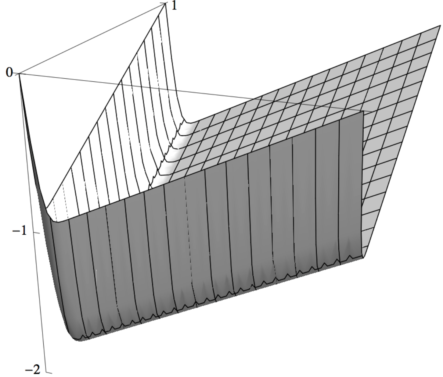
(7.2) u⁡(x,y)=x+y−Erf⁡(x/2​ε)+Erf⁡(y/2​ε)Erf⁡(1/2​ε)u(x,y)=x+y-\frac{{\mathrm{Erf}}\left(x/\sqrt{2\varepsilon}\right)+{\mathrm{Erf}}\left(y/\sqrt{2\varepsilon}\right)}{{\mathrm{Erf}}\left(1/\sqrt{2\varepsilon}\right)}

where Erf{\mathrm{Erf}} is the error function defined by Erf⁡(x)=2π​∫0xe−t2​𝑑t{\mathrm{Erf}}(x)=\frac{2}{\sqrt{\pi}}\int_{0}^{x}{\text{e}^{-t^{2}}}{\,\mathrm{d}t}. For 0<ε≪10<\varepsilon\ll 1 this problem exhibits an exponential boundary layer along the outflow boundaries x=0x=0 and y=0y=0 of width 𝒪⁡(ε){\mathcal{O}(\sqrt{\varepsilon})}.

Away from the layers the boundary conditions on the inflow boundaries x=1x=1 and y=1y=1 are well approximated by y−1y-1 and x−1x-1 respectively. The hyperbolic solution with these boundary conditions is given by u0​(x,y)=x+y−2u_{0}(x,y)=x+y-2. This gives

(7.3) uε​(x,y)=2−Erf⁡(x/2​ε)+Erf⁡(y/2​ε)Erf⁡(1/2​ε).u_{\varepsilon}(x,y)=2-\frac{{\mathrm{Erf}}\left(x/\sqrt{2\varepsilon}\right)+{\mathrm{Erf}}\left(y/\sqrt{2\varepsilon}\right)}{{\mathrm{Erf}}\left(1/\sqrt{2\varepsilon}\right)}.

We plot (7.2) and (7.3) for ε=10−3\varepsilon=10^{-3} in Figure 7.1; note that away from the layers the solution uεu_{\varepsilon} is close to zero.

We let ΩcG{\Omega_{\textrm{cG}}} be a set of the type (1−δ,1)2(1-\delta,1)^{2}, 0<δ<10<\delta<1. For each δ\delta the supremum

supε∈(0,εmax]∥uε∥H2​(ΩcG)\sup_{\varepsilon\in(0,\varepsilon_{\mathrm{max}}]}\lVert u_{\varepsilon}\rVert_{H^{2}({\Omega_{\textrm{cG}}})}

is finite. The dependence of ∥uε∥H2​(ΩcG)\lVert u_{\varepsilon}\rVert_{H^{2}({\Omega_{\textrm{cG}}})} with respect to δ\delta and to ε\varepsilon is illustrated in Figure 7.2.

Figure 7.2: ∥uε∥H2​(ΩcG)\lVert u_{\varepsilon}\rVert_{H^{2}({\Omega_{\textrm{cG}}})} for different values of δ\delta.
Figure 7.3: Difference between cdG and dG solutions.

For this example c−12∇⋅b=1c-{\frac{1}{2}}\nabla\cdot{b}=1, so Assumption 2.9 is satisfied. Further, we fix ε=10−6\varepsilon=10^{-6} and consider uniform square meshes of edge length 2−52^{-5} so that Assumption 2.12 is also satisfied as the smallest local mesh Péclet number being 488.28488.28.

We define 𝒯cG=[1−δh,1]2{\mathcal{T}_{{\textrm{cG}}}}=[1-\delta_{h},1]^{2}, where δh=m​2−5\delta_{h}=m2^{-5}, m∈{0,…,32}m\in\{0,\ldots,32\}. Note that, having fixed the mesh, δh\delta_{h} is a discrete parameter. The interface JJ is composed of the edges lying on the lines y=δhy=\delta_{h} for x≥δhx\geq\delta_{h} and x=δhx=\delta_{h} for y≥δhy\geq\delta_{h}. The smallest value of b⋅n{{b}\cdot n} is δh\delta_{h} occuring on the edges containing the point (δh,δh)(\delta_{h},\delta_{h}). Thus, in this case, Assumption 2.33 reads 14​m​h>ε​σh3/2\frac{1}{4}mh>\varepsilon\frac{\sigma}{h^{3/2}} and is satisfied for all m∈{1,…,32}m\in\{1,\ldots,32\} (note that this assumption is trivially satisfied when m=0m=0) for this choice of ε\varepsilon and hh if σ<200\sigma<200; in the shown computations σ=10\sigma=10.

In Figure 7.3 we plot the L2​(Ω){L^{2}(\Omega)} norm, ε\sqrt{\varepsilon} weighted H1​(𝒯h){H^{1}({\mathcal{T}_{h}})} semi-norm, and L2L^{2} norm of the jumps on ℰh{\mathcal{E}_{h}}(represented by ⟦⋅⟧\llbracket\,\cdotp\rrbracket) for both the difference in the dG and cdG approximations and the error in the cdG approximation. Note from Figure 7.3 that the difference in the approximations increases only very slowly until the final data points (where 𝒯cG≈𝒯h{\mathcal{T}_{{\textrm{cG}}}}\approx{\mathcal{T}_{h}}). When the continuous region covers the layer, non-physical oscillations pollute the approximation in function of δh\delta_{h}.

In Table 7.1 we show the number of degrees of freedom (dofs) as the continuous region is increased. Reducing the degrees of freedom to approximately 30% of the dG method degrees of freedom results in only a very slight difference in the norm, thus showing that a considerable saving can be made without compromising stability.

1−δ1-\delta dofs % of dG dofs ε​∥∇h(wh−vh)∥H1​(Ω)\sqrt{\varepsilon}\lVert{\nabla_{h}}(w_{h}-v_{h})\rVert_{H^{1}(\Omega)}
dG 4096 100 0.0
8×2−58\times 2^{-5} 3361 82.1 3.1157e-08
16×2−516\times 2^{-5} 2417 59.0 6.8911e-08
24×2−524\times 2^{-5} 2121 51.8 8.7544e-08
30×2−530\times 2^{-5} 1457 35.6 1.7934e-07
31×2−531\times 2^{-5} 1276 31.2 2.7896e-07
cG 1089 26.6 1.2444e-02
Table 7.1: Degrees of freedom with ε=10−6\varepsilon=10^{-6}.

We finally remark that, at least for the example considered here, the choice of 𝒯cG{\mathcal{T}_{{\textrm{cG}}}} leaving one layer of elements at the outflow boundary is optimal. Indeed, adding even a single element to the 𝒯cG{\mathcal{T}_{{\textrm{cG}}}} region results in oscillations polluting the solution. For example, for

𝒯cG=[2−5,1]2∪([0.5,0.5+2−5]×[0,2−5]),{\mathcal{T}_{{\textrm{cG}}}}=[2^{-5},1]^{2}\cup([0.5,0.5+2^{-5}]\times[0,2^{-5}]),

i.e., adding a sinlge element to 𝒯cG{\mathcal{T}_{{\textrm{cG}}}} halfway along the xx-axis, results in

∥wh−vh∥L2​(Ω)\displaystyle\lVert w_{h}-v_{h}\rVert_{L^{2}(\Omega)} =4.7966×10⁻²,\displaystyle=4.7966\times 10^{-2},
ε​∥∇h(wh−vh)∥L2​(Ω)\displaystyle\sqrt{\varepsilon}\lVert{\nabla_{h}}(w_{h}-v_{h})\rVert_{L^{2}(\Omega)} =4.5008×10⁻³,\displaystyle=4.5008\times 10^{-3},

a significant increase on the norms for 𝒯cG=[2−5,1]2{\mathcal{T}_{{\textrm{cG}}}}=[2^{-5},1]^{2}. Notice that this choice of 𝒯cG{\mathcal{T}_{{\textrm{cG}}}} violates Assumption 2.33.

8 Acknowledgements:

We gratefully thank the Archimedes Center for Modeling, Analysis and Computation in Crete for hosting the authors during the preparation of this manuscript.

References

  • [1] D. N. Arnold, F. Brezzi, B. Cockburn, and L. D. Marini, Unified analysis of discontinuous Galerkin methods for elliptic problems, SIAM Journal on Numerical Analysis, 39 (2001), pp. 1749–1779.
  • [2] B. Ayuso and L. D. Marini, Discontinuous Galerkin methods for advection-diffusion-reaction problems, SIAM Journal on Numerical Analysis, 47 (2009), pp. 1391–1420.
  • [3] C. Bardos and J. Rauch, Maximal positive boundary value problems as limits of singular perturbation problems, Transactions of the American Mathematical Society, 270 (1982), pp. pp. 377–408.
  • [4] R. Becker, E. Burman, P. Hansbo, and M. Larson, A reduced P1-discontinuous Galerkin method, tech. rep., EPFL, 2004. EPFL-IACS report 05.2004.
  • [5] A. Buffa, T. J. R. Hughes, and G. Sangalli, Analysis of a multiscale discontinuous Galerkin method for convection-diffusion problems, SIAM Journal on Numerical Analysis, 44 (2006), pp. 1420–1440.
  • [6] A. Cangiani, J. Chapman, E. H. Georgoulis, and M. Jensen, On local super-penalization of interior penalty Galerkin methods, submitted jounral article, (2012).
  • [7] A. Cangiani, E. H. Georgoulis, and M. Jensen, Continuous and discontinuous finite element methods for convection-diffusion problems: A comparison, in International Conference on Boundary and Interior Layers, Göttingen, July 2006.
  • [8] B. Cockburn, G. Karniadakis, and C. Shu, The development of discontinuous Galerkin methods, in Discontinuous Galerkin Methods: Theory, Computation, and Applications, B. Cockburn, G. Karniadakis, and C. Shu, eds., vol. 11 of Lecture Notes in Computational Science and Engineering, Springer, 2000.
  • [9] B. Cockburn and C.-W. Shu, The local discontinuous Galerkin method for time-dependent convection-diffusion systems, SIAM Journal on Numerical Analysis, 35 (1998), pp. 2440–2463.
  • [10] C. Dawson and J. Proft, Coupling of continuous and discontinuous Galerkin methods for transport problems, Computer Methods in Applied Mechanics and Engineering, 191 (2002), pp. 3213 – 3231.
  • [11] P. R. B. Devloo, T. Forti, and S. M. Gomes, A combined continuous-discontinuous finite element method for convection-diffusion problems, Latin American Journal of Solids and Structures, 2 (2007), pp. 229–246.
  • [12] A. Ern and J.-L. Guermond, Theory and Practice of Finite Elements, Springer-Verlag, New York, 2004.
  • [13] I. Perugia and D. Schötzau, On the coupling of local discontinuous Galerkin and conforming finite element methods, Journal of Scientific Computing, 16 (2001), pp. 411–433.
  • [14] H.-G. Roos, M. Stynes, and L. Tobiska, Numerical Methods for Singularly Perturbed Differential Equations: Convection-Diffusion and Flow Problems, Springer-Verlag, Berlin, Second ed., 2008.
  • [15] L. R. Scott and S. Zhang, Finite element interpolation of nonsmooth functions satisfying boundary conditions, Mathematics of Computation, 54 (1990), pp. 483–493.