Multiple path adiabatic crossing in a 3 site ring
Abstract
We find an exact expression for the current that is induced in a 3 site ring during a multiple-path adiabatic crossing. The understanding of the dynamics requires to go beyond the two-level phenomenology. In particular we highlight a prototype process, “adiabatic metamorphosis”, during which current is flowing through a non-accessible site. This helps to understand the crossover from coherent non-classical splitting to stochastic noisy-alike partitioning of the current.
1 Introduction
Adiabatic quantum transport [1, 2, 3, 4, 5] is a major theme in quantum mechanics, with diverse applications, e.g. quantum Hall effect [6], dynamics of Josephson junctions [7], and the analysis of pericyclic reactions [8]. If a parameter is slowly varied in a closed system that has a non-trivial topology, say a ring shaped device, the formalism implies that current is induced. In the absence of magnetic fields we call such an effect “quantum stirring” [9, 10, 11, 12]. On the one hand it is related to the classical problem of “stochastic stirring” [13, 14, 15, 16], and on the other hand it is related to “quantum pumping” in open systems [17, 18, 19, 20, 21, 22, 23, 24].
Most results regarding adiabatic quantum transport are rather abstract, based on a formal mathematical approach, notably the “Dirac monopoles picture” [4, 9]. This should be contrasted with the analysis of stochastic stirring where the phenomenology is quite mature [13]. The way to gain better physical insight is to analyze prototype model systems [11, 12], and to identify the elementary ingredients that determine the nature of the dynamics.

In the present work we would like to address the minimal model for a closed isolated quantum system that has a non-trivial topology. This is evidently the 3 site ring that is illustrated in Fig. 1. Quite generally, in the absence of magnetic field, the stationary states of the system, and the ground state in particular, carry zero current. If we want to get current we have to drive the system by varying a parameter in time. In the adiabatic limit the current is given by the following formula
| (1) |
where is the geometric conductance:
| (2) |
In the above formula is the adiabatic ground state that depends on the parameter , and on an auxiliary test flux through the bond of interest.
Specifically we want to consider the following scenario, which we call “Multiple path adiabatic crossing”. Assume that a particle is placed in the 0th site, which we call “dot”. The potential of the dot is raised slowly from to . As a result the particle is adiabatically transferred from the dot to the other two sites. These two sites (”1” and ”2”) can be regarded as a two-orbital entity that we call “wire”. At the end of the process the particle will be found in the lower energy level of the wire. We ask what is the current through the first bond (). Equivalently we can characterize the transport by the integrated current
| (3) |
In particular we define . If we had single-path geometry obviously the result for the latter would be , reflecting 100% transition probability. But we are dealing here with a multiple path geometry.
At this point it is important to emphasize that if we were dealing with a stochastic process the current would be partitioned between the paths, hence . But the essence of “quantum stirring” is the observation that during the driving process a circulating current is induced. Due to this circulation, the integrated current can be any number.
The above recipe Eq. (2) for calculating adiabatic currents is well known from the works on adiabatic transport, but its physical implications have not been fully recognized. In fact the original interest in this model has been motivated by a wrong assertion that “adiabatic pumping” in a closed system has to be quantized [27]. The fallacy of this statement has been illuminated using the “Dirac monopoles picture” [9] and later using a 2 level “splitting ratio” phenomenology [12, 28]. The exact solution of the 3 site ring has been considered as well [9], to establish that of a closed driving cycle can have any value. However, the full solution of the multiple-path adiabatic crossing has not been explored. In particular it has remained vague whether to go beyond the two level approximation is of any physical significance.
Outline.– We first derive an exact expression for . This is quite straightforward, but as usual the exact expression is not very illuminating physically. We therefore try to derive approximations that are based on a two-level phenomenology. Then we realize that there are different regimes depending on the ratio between the inter dot-wire and the intra-wire couplings. In particular we find a regime where the crossing process involves an “adiabatic metamorphosis” stage, during which current is flowing through the energetically non-accessible dot.
2 for a 2-site system
We start with the analysis of a single-path crossing in a 2 site system. The Hamiltonian and the associated current operator are
| (4) |
where is the potential of the dot, and is the level that is crossed, and is the dot-level coupling. The extra parameter is reserved for later. Without loss of generality we assume to be real and positive . For the purpose of defining the current operator , and later using Eq. (2), one should substitute .
For a given value of the energy of the adiabatic ground state is
| (5) |
The corresponding eigenstate is
| (6) |
where the normalization factor for zero flux is
| (7) |
Using Eq. (2) we get
| (8) |
leading to
| (9) |
where . It is easily verified that upon integration , hence , as implied by the continuity equation for a single-path adiabatic crossing.
3 for a 3-site system
We now use the same procedure for the analysis of the double-path crossing in a 3 site system. The Hamiltonian and the associated current operator are
| (10) |
We assume the s to be real (no magnetic field) but for the purpose of defining the current through the bond, and later using Eq. (2), we substitute .
The secular equation for the eigenvalues is
| (11) |
with the solution
| (12) |
where
| (13) | |||||
| (14) | |||||
| (15) |
As is varied from to , the angle varies from to , and the ground state energy goes from to . The corresponding eigenstates are
| (16) |
The normalization factor for zero flux is
| (17) | |||||
| (18) |
If we placed the test flux at the bond we would get from Eq. (2) the result that had been derived in [9] for the current in the bond, namely:
| (19) |
But our interest is in the current that goes through the bond. Accordingly we have placed the test flux at and get
| (20) | |||
| (21) |
4 The integrated current
On the basis of Eq. (21) one observes that for any the integrated current Eq. (3) at the end of the process is
| (22) |
Strangely enough this does not depend on the value of . But for , based on the same expression, the result is quite different:
| (23) |
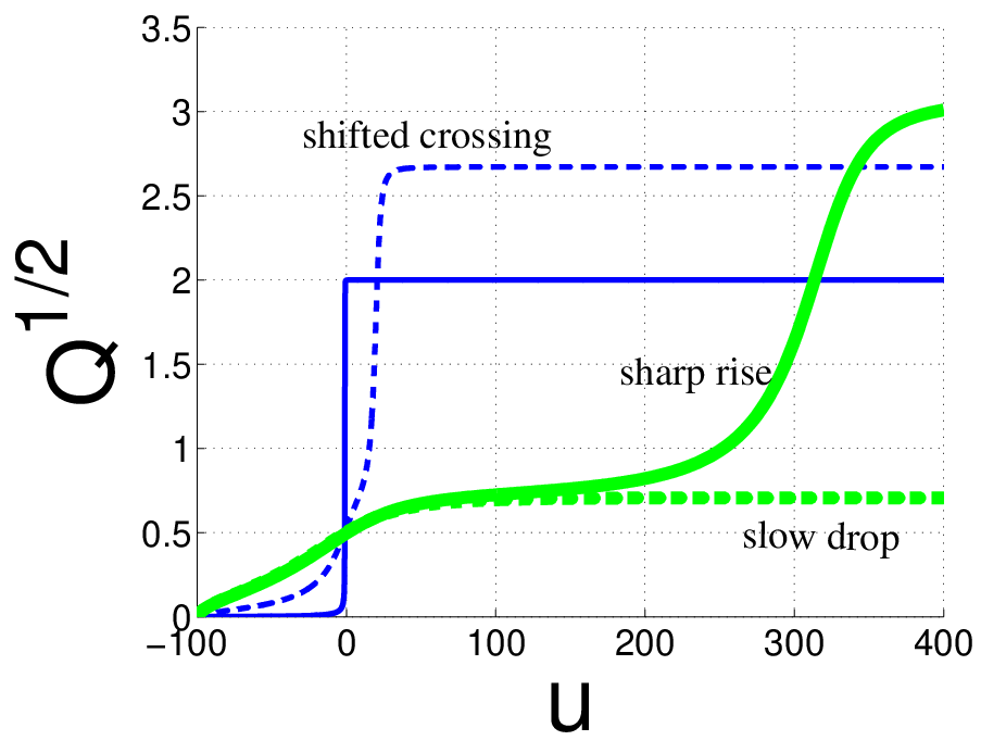
It is therefore required to explain what happens physically if is very very small but not zero. In Fig. 2 we illustrate for several representative cases. If is large rises monotonically in a step-like fashion to the value that is predicted by Eq. (22). However if is small one observes two stages in the parametric evolution: first rises to the value that is predicted to Eq. (23), and only after that it re-adjust to the value of Eq. (22). In Section 9 we shall use the term “adiabatic metamorphosis” in order to describe this re-adjustment of the occupations. We shall see that it involves a much larger parametric scale that diverges in the limit . Hence for we are left with Eq. (23) instead of Eq. (22). A closer inspection of the metamorphosis stage (dashed vs solid green curves in Fig. 2) reveals that it can be either a gradual or a sharp transition, depending on the relative sign of and .
The values for the illustrations in Fig. 2 are indicated in the diagram of Fig. 3. In the following sections we would like to illuminate the different regions in this diagram by attempting a two-level approximation scheme.

5 The 2-level approximation
Let us try to reduce the 3 level dynamics to a 2 level crossing problem. For this purpose we switch to the following basis:
| the dot state | (24) | ||||
| (25) | |||||
| (26) |
In the new basis the Hamiltonian and the current operator Eq. (10) take the following form:
| (27) |
with couplings
| (28) |
Without loss of generality we focus on the strongest bond, meaning that we assume , and by appropriate gauge we arrange that , hence both are positive numbers. We shall see that a two-level approximation scheme is useful for the treatment of 3 cases that are indicted in Fig. 3, namely
| (29) | |||
| (30) | |||
| (31) |
In all these cases we can fit the exact result Eq. (21) to the two-level expression Eq. (9), with some effective values for and and . The remaining case of having a relatively small but finite is excluded, because it cannot be treated within the framework of a two level approximation. This last case will be considered separately.
6 The simple 2-level approximation
We first consider the very simple case, in which the third (upper) level can be ignored. The condition for that is . Taking the relevant block from the Hamiltonian of Eq. (27) one obtains a reduced Hamiltonian that is given by Eq. (4) with the effective parameters
| (32) |
Hence we deduce that of Eq. (9) can be used as an approximation for the exact result. This expectation is confirmed in Fig. 4.
The presence of reflects that the flow is via two bonds instead of via only a single bond, unlike the case of the 2-sites model. In other words the particle “splits” and flows through both bonds. We notice that the integrated current can have a manifestly non-classical value: it can be either larger than 1 or negative. In fact, if it is larger than 1 in one bond it has to be negative in the other bond, since the total corresponds to 100% probability of being adiabatically transferred. The non-classical value of reflects a circulating current that is induced during the transition. In a semi-classical language it means that the particle is looping several rounds through the ring before ending up in the wire.
7 The shifted 2-level approximation
The simple two-level approximation of the previous section is not valid if . Still if we can still get a result that looks like Eq. (9). The solution procedure involves two steps. In the first step we switch to a new basis:
| (33) | |||||
| (34) | |||||
| the lower (odd) wire state | (35) |
where
| (36) |
In this basis the block of the Hamiltonian Eq. (27) that contains the strongly interacting states and becomes diagonal. Now it is possible to neglect the upper level and we get a two-level crossing problem that involves the “dressed” dot level and the lower (odd) wire level . The adiabatic energy of the former is
| (37) |
while that of the latter is . Accordingly the shifted crossing point is
| (38) |
The stronger the coupling to the upper level, the larger is the shift of .
In order to estimate the effective parameters of the shifted two level crossing we have to write the Hamiltonian and the current operator in the new basis. In the vicinity of the crossing point we set , getting
| (39) |
and
| (40) |
where is the same as in the previous section. It is important to realize that up to constant the effective dot potential equals with . It is not difficult to see that this implies the replacement
| (41) |
Hence within the framework of the two level approximation the effective in Eq. (9) is not but rather it should be divided by . So eventually we deduce that the can be approximated by Eq. (9) with an effective coupling parameter
| (42) |
This expectation is confirmed in Fig. 4. Note again that is the same as in the simple two-level approximation, and that we evaluate at the crossing point using Eq. (36) with Eq. (38).
(a1)  (a2)
(a2) 
(b1)  (b2)
(b2) 
8 Adiabatic crossing for
In the previous versions of the two-level approximation, the intra-wire coupling was large in some sense. Now we go to the other extreme limit of having . This resembles the standard setup that is used in the analysis of stimulated Raman adiabatic passage (STIRAP). In fact we can adopt here the same “dark state” picture in order to reduce the problem to a two-level crossing. Namely, for this purpose we switch to the following basis:
| the dot state | (43) | ||||
| (44) | |||||
| (45) |
In the new basis the state decouples, and hence we end up again with a reduced Hamiltonian that is given by Eq. (4) with the effective parameters
| (46) |
Hence we deduce that of Eq. (9) with the above set of effective parameters coincides in this case with the exact result.
It should be clear that for we no longer have a non-trivial geometry, and hence a circulating current cannot be induced. For this reason it is a-priori expected to get an effective two-level description with . In fact we got for a stochastic look-alike expression that reflect the relative transmission of the two bonds.
(a) 
(b) 
(c) 
9 Adiabatic metamorphosis
Let us contrast the case with the case. The two cases give very different results. We would like to better clarify what really happens if is very small. We first recall the optional bases for the representation of the system. The standard basis is . The wire-eigenstates basis is , and the basis is . For the instantaneous eigenstates we shall use the notations , and and .
Recall that for the dark state decouples, meaning that , while the other two eigenstates and are superpositions of and . At the end of an adiabatic process the system will be found in the degenerate state. However, if is non-zero, the system ends up in the non-degenerate state.
It is therefore clear that for very small but finite the adiabatic ground-state changes from to . We call this “adiabatic metamorphosis”. We define as the value of at which this metamorphosis occurs. Close to the dot level is energetically far above, hence the lower states and form a 2-level system with virtual coupling through the distant dot level. The reduced Hamiltonian is determined by 2nd order perturbation theory:
| (47) |
By inspection of this Hamiltonian it is clear that for large enough the direct coupling takes over, and then the metamorphosis to is finalized. In particular it is interesting to consider the case in which . Then the metamorphosis crossing point is sharply defined:
| (48) |
which is demonstrated in Fig. 5. Otherwise the metamorphosis is a gradual process, as was illustrated in Fig. 2. Note that for sharp metamorphosis, at , all the probability is concentrated in one site of the wire, namely, in the site that is more strongly connected to the dot. This is demonstrated in panel (c) of Fig. 5.
10 Beyond the adiabatic limit
In order for the process to be adiabatic the probability distribution should change slowly with time. This implies that the current cannot be very large. Let us see what is the precise statement. Specifically for a two level Landau-Zener crossing the adiabatic condition is
| (49) |
where is the coupling between the dot and the crossed level. This implies that
| (50) |
One observes that the maximal current reflects the coupling. Furthermore, also the integrate current cannot be too large. It is simply bounded by unity () reflecting that the maximum transfer is 100%.
If we consider multiple path geometry it is easy to show that the conclusion regarding the maximal current still holds. However, as was clarified in previous section, the integrated current becomes arbitrarily large if , rather than being bounded. A large value reflects the existence of a circulating current that is induced in the system during the driving process. It should be clear that in order to witness one has to satisfy a very demanding adiabatic condition, because the effective coupling that enters into Eq. (49) is .
Within the conventional framework of the two-level approximation, the implication of non-adiabaticity is to have less than 100% probability to cross from the dot to the wire, as implied by the Landau-Zener expression [25, 26]. But for very small , such that the metamorphosis scenario applies, the implications of non-adiabaticity are more interesting as explained below.
For finite there is a finite range of small values for which the result for is approximately the same as for . The complementary statement is as follows: for a given , if is large enough, the system does not have enough time to realize that it is coupled to a “dark state”. Roughly this non-adiabatic condition takes the form . Thus we have an intermediate “diabatic” regime where the dynamics is “adiabatic” with regard to the crossing, but “sudden” with regard to the metamorphosis. The bottom line of the above discussion is illustrated in Fig. 5. One observes that for mild values of the metamorphosis stage is not expressed, and the dynamics looks like that of system.
11 Discussion
Transport in quantum networks is a theme that emerges in diverse contexts. The simplest network that has non-trivial topology is the 3 site system that we have considered in this paper. It can be regarded as composed of “dot” and “wire” segments. The most elementary process that has to be understood is an adiabatic sweep of the potential energy of a selected site (the dot), leading to transfer of the probability to the other sites (the wire). Unlike stochastic process in which the probability current is partitioned with branching ratios that are bounded within , here the splitting ratio can be any number reflecting a quantum stirring effect.
The detailed analysis of the 3 sites model allows to highlight several essential ingredients in the analysis of quantum transport. In particular it was important to clarify what is the way in which the two-level approximation breaks down. Strangely enough the splitting ratios are independent of the intra-wire coupling, but still the line shape is strongly influenced.
In particular we have distinguished between two type of processes: inter dot-wire “adiabatic crossing” processes; and intra-wire “adiabatic metamorphosis” processes. In the former probability is transported between the dot and the wire, while in the latter the changes in the occupation are exclusively within the wire. During the metamorphosis stage the dot level is very far from the wire levels, but still current flows through the inter-connecting bonds, without being accumulated in the dot.
We believe that the processes that we have illuminated are of much relevance, and might shed new light, on the analysis of pericyclic reactions [8]. In this context the method of calculating electronic quantum fluxes had assumed that the latter can be deduced from the continuity equation. Such procedure is obviously not applicable for (say) a ring-shaped molecule: due to the multiple path geometry there is no obvious relation between currents and time variation of probabilities.
Furthermore, it is important to understand how non-adiabaticity and decoherence affect adiabatic transport. Possibly the most dramatic demonstration concerns the suppression of metamorphosis processes by mild non-adiabaticity. Then we get instead of coherent splitting, stochastic-like partitioning of the current. The reason for this crossover can be optionally explained using a very general paradigm. Namely, once the intra-wire couplings are introduced, there is a protecting “gap” that becomes effective if the rate of the sweep is slow enough; this protecting gap forces the particle to be in a definite superposition at any moment. It follows that coherent splitting, unlike “partitioning” of current is not a noisy process. This observation has implications on the calculation of “counting statistics” and “shot noise” [29, 28].
References
References
- [1] D.J. Thouless, Phys. Rev. B 27, 6083 (1983).
- [2] Q. Niu and D. J. Thouless, J. Phys. A 17, 2453 (1984).
- [3] M.V. Berry, Proc. R. Soc. Lond. A 392, 45 (1984).
- [4] J.E. Avron, A. Raveh and B. Zur, Rev. Mod. Phys. 60, 873 (1988).
- [5] M.V. Berry and J.M. Robbins, Proc. R. Soc. Lond. A 442, 659 (1993).
- [6] J.E. Avron, D. Osadchy, R. Seiler, Physics Today 56, 38 (2003).
- [7] M. Mottonen, J.P. Pekola, J.J. Vartiainen, V. Brosco, F.W.J. Hekking, Phys. Rev. B 73, 214523 (2006͒).
- [8] D. Andrae, I. Barth, T. Bredtmann, H.-C. Hege, J. Manz, F. Marquardt, and B. Paulus, J. Phys. Chem. B, 115, pp 5476 (2011).
- [9] D. Cohen, Phys. Rev. B 68, 155303 (2003).
- [10] D. Cohen, T. Kottos, H. Schanz, Phys. Rev. E 71, 035202(R) (2005).
- [11] G. Rosenberg and D. Cohen, J. Phys. A 39, 2287 (2006).
- [12] I. Sela, D. Cohen, J. Phys. A 39, 3575 (2006); Phys. Rev. B 77, 245440 (2008).
- [13] S. Rahav, J. Horowitz, C. Jarzynski, Phys. Rev. Lett., 101, 140602 (2008).
- [14] D. A. Leigh, J.K.Y. Wong, F. Dehez, F. Zerbetto, Nature (London) 424, 174 (2003)
- [15] J.M.R. Parrondo, Phys. Rev. E 57, 7297 (1998)
- [16] R.D. Astumian, Phys. Rev. Lett. 91, 118102 (2003).
- [17] M. Buttiker, H. Thomas, A Pretre, Z. Phys. B Cond. Mat. 94, 133 (1994).
- [18] P. W. Brouwer, Phys. Rev. B 58, R10135 (1998)
- [19] B.L. Altshuler, L.I. Glazman, Science 283, 1864 (1999).
- [20] M. Switkes, C.M. Marcus, K. Campman, A.C.Gossard Science 283, 1905 (1999).
- [21] J.A. Avron, A. Elgart, G.M. Graf, L. Sadun, Phys. Rev. B 62, R10618 (2000).
- [22] D. Cohen, Phys. Rev. B 68, 201303(R) (2003).
- [23] L.E.F. Foa Torres, Phys. Rev. Lett. 91, 116801 (2003); Phys. Rev. B 72, 245339 (2005).
- [24] O. Entin-Wohlman, A. Aharony, Y. Levinson, Phys. Rev. B 65, 195411 (2002).
- [25] C. Zener, Proc. R. Soc. Lond. A 317, 61 (1932).
- [26] N.V. Vitanov, B.M. Garraway, Phys. Rev. A 53 4288 (1996).
- [27] T.A. Shutenko, I.L. Aleiner and B.L. Altshuler, Phys. Rev. B61, 10366 (2000).
- [28] M. Chuchem, D. Cohen, J. Phys. A 41, 075302 (2008); Phys. Rev. A 77, 012109 (2008); Physica E 42, 555 (2010).
- [29] L.S. Levitov, G.B. Lesovik, JETP Lett. 58, 230 (1993͒); Y.V. Nazarov, M. Kindermann, Eur. Phys. J. B 35, 413 (2003͒).