Multilevel simulation of functionals of Bernoulli random variables with application to basket credit derivatives
Abstract
We consider Bernoulli random variables, which are independent conditional on a common random factor determining their probability distribution. We show that certain expected functionals of the proportion of variables in a given state converge at rate as . Based on these results, we propose a multi-level simulation algorithm using a family of sequences with increasing length, to obtain estimators for these expected functionals with a mean-square error of and computational complexity of order , independent of . In particular, this optimal complexity order also holds for the infinite-dimensional limit. Numerical examples are presented for tranche spreads of basket credit derivatives.
Key words: Multilevel Monte Carlo simulation, large deviations principle, exchangeability, basket credit derivatives
1 Introduction
This article is concerned with the efficient numerical estimation of expectations of functionals of a large number, , of exchangeable Bernoulli random variables. The objective of this work is thus two-fold: to analyse the order of convergence in of expected functionals as tends to infinity, and to derive estimators for these expectations for which the computational complexity is asymptotically independent of .
We begin by analysing the convergence in the case of general Lipschitz and smooth functions, , of the average of exchangeable Bernoulli random variables as goes to infinity. We then consider the case when has a certain piecewise linear structure and show that the convergence order is the same as in the smooth case. These results are relevant, for instance, if one wants to approximate the result for large but finite by its limit. A number of applications come from the credit risk literature. In [14], Vasicek derives an expression for the limiting distribution of portfolio losses in a Normal factor model, where default of a firm is indicated by its value process being below a default barrier at maturity of the debt. In the large portfolio limit, the randomness comes solely from a common market factor, while a law of large numbers holds for idiosyncratic components conditionally on this factor. Bush et al., in [5], extend this to a dynamic set-up where it is seen that the density of the limit empirical measure of firm values satisfies a stochastic partial differential equation (SPDE) and can be used to approximate tranche spreads of basket credit derivatives; [4] gives an extension to jump diffusion models while [9] include extensions to heterogeneity and self-exciting defaults rendering the resulting equations non-linear. Further studies focus particularly on the tail of the limiting loss distribution, see [7], [12] and the references therein.
A driving practical motivation for investigating the limiting behaviour is that the original sequence of random variables is costly to simulate, because of the large number of underlying processes, often required over large time horizons. Moreover, often many Monte Carlo samples are necessary for sufficiently accurate estimation of, for instance, expected tranche losses of credit basket. This paper takes a different tack and develops a simulation method where the computational complexity is asymptotically independent of . A small tweak of the algorithm can also be used to approximate the limit obtained when goes to infinity.
More concretely, it turns out that an interpretation of the multi-level Monte Carlo approach (see [11]) in the present context allows us to construct estimators based on sequences with increasing lengths and a number of samples which decreases faster than the length increases, such that the overall computational complexity is essentially no larger than for fixed small .
A conceptually similar though distantly related approach is used in [3], where the multilevel idea is applied to a sequence of martingales to estimate a dual upper bound for the value of an early exercise option. In that setting they are able to show, as we do here, that the achievable complexity is not substantially larger than that of a non-nested simulation. The general problem of estimating conditional expectations through nested multilevel simulation is addressed in [6]. There, further extrapolation is used to reduce the bias of estimators, while here we will propose an improved estimator which reduces the variance of higher level estimators.
This article is organised as follows. In Section 2, we introduce the setting and outline the main convergence results, explaining how they can be used to construct efficient estimators. The first key result on the convergence order of expected functionals is proved in Section 3, with numerical illustrations from an example of a basket credit derivative presented in Section 4. In Section 5, we introduce in detail two multilevel simulation methods and derive bounds on their computational complexity to achieve a prescribed accuracy. Finally, in Section 6 we present numerical results illustrating the efficiency gains achieved through multilevel simulation in this context and Section 7 discusses possible extensions.
2 Set-up and main results
In this article, we are concerned with the behaviour of “loss” variables describing the fraction of random variables in a certain state, and expected functionals of this loss variable, as goes to infinity. The application we have in mind, and for which we will present numerical illustrations, is that of a basket of defaultable firms, and then the loss is the fraction of firms which default over a certain period.
More precisely, on a probability space , consider a sequence of Bernoulli random variables , , and a random variable taking its values in . If required we write where canonically we could take and . The probability measure is constructed as follows. The random variable is generated according to its marginal law and then, conditional on , the -algebra generated by , the are independent random variables with law given by
| (2.1) |
To re-iterate, the Bernoulli random variables are conditionally independent given a common factor. Thus for each
where . We will often write for the conditional law of the given and for the associated conditional expectation. In the setting of defaultable firms, iff the -th firm defaults, and is a global factor modelling the common tendency of firms to default. We define the loss variable to be the proportion of Bernoulli variables in state 1
| (2.2) |
We consider a Lipschitz function and random variables and defined as
| (2.3) | |||||
| (2.4) |
In particular, we will study of the form
where denotes the positive part and are constants. In credit derivative pricing, the particular shape of the function in (2) measures the losses in a certain tranche with attachment point and detachment point , and its expectation is the building block for formulae for CDO tranche spreads. A typical CDO pool consists of firms, while typical loan or mortgage books can have substantially more obligors, and it is therefore practically relevant to understand the behaviour of expected functionals for large and to devise computationally efficient estimators.
By a conditional version of the strong law of large numbers and the continuity of
| (2.9) | |||||
| (2.10) |
This convergence will also hold in (see Lemma 3.1).
We study here the convergence rate of and will prove the following two results. The first statement for Lipschitz and smooth functions is a relatively straightforward consequence of (2.1) and the easily computable convergence rate of . The second result shows that for a specific which is only piecewise smooth we can still obtain the same convergence order as in the smooth case and with explicitly computable bounds.
Theorem 2.1.
Theorem 2.2.
For defined in (2), if the cumulative density function (CDF) of is Lipschitz at and with Lipschitz constant , i.e.,
| (2.14) |
for and all , then
Note that if has a density function which is bounded, then the CDF is certainly Lipschitz. The fact that we only need the Lipschitz property at and will be useful for the applications considered later.
Taking the two Theorems together, order 1 for the convergence of expectations also follows for piecewise smooth which are Lipschitz overall, provided is Lipschitz.
These Theorems show that expected functionals for large or infinite can be successively approximated by those with smaller . Combining this with a control variate idea leads to multilevel simulation with a substantial variance reduction for large . Specifically, the above results imply that for Lipschitz we have and for any positive integer with some constants and . We can consider a sequence , , with corresponding and . Translating the central idea in [11] to this setting, we use the decomposition
| (2.15) |
and estimate every summand separately by defining estimators
| (2.16) |
where ‘c’ denotes a ‘coarse’ estimator on level , i.e., using only instead of Bernoulli random variables, precisely,
| (2.17) | |||||
| (2.18) |
where , , are independent samples of for fixed level and independent across levels. They are constructed from a loss factor (with the same distribution as , independent across and ) in the same way that is constructed from .
The number of samples on each level, , can be chosen to obtain an optimal allocation of computational cost for a given overall mean-square error (MSE). The general construction in [11] immediately gives the following result.
Proposition 2.1 (cf. [11], Theorem 3.1).
Let , as above. If there exist independent estimators based on Monte Carlo samples, and positive constants such that and
- i)
- ii)
- iii)
- iv)
where is the computational complexity of
then there exists a positive constant such that for any there are values and for which the multilevel estimator
| (2.19) |
has a mean-square-error with bound
with a computational complexity with bound
The above result is meaningful only in situations where it is not possible or practical to sample from directly, as otherwise could be computed with complexity in the standard Monte Carlo way.
Moreover, in some situations it is not which is of interest, but for large but finite , and then it is essential to have a method to estimate in a complexity which does not increase sharply in .
For instance, take given and estimate with the standard (i.e., single level) Monte Carlo estimator
where is the number of samples and the , for different , are independent samples of . Then and , where it follows from
under the conditions of either Theorem 2.1 or Theorem 2.2, that
for sufficiently large and some constants independent of . That is to say, the variance of and subsequently that of the estimator is bounded below with a positive number independent of . Hence, if a MSE of is required for , the complexity is
i.e., increases (at least) linearly in . (A similar argument shows that this is also an upper bound.)
If one wants to use not as an estimator to but , a bias occurs and
assuming the bias is of order as in Proposition 2.1. To reduce the bias and hence the error, has to be increased simultaneously with . More precisely, for MSE it is optimal to choose and , leading to a computational complexity
The following Corollary addresses both cases of large finite and infinite and improves on the convergence rates of the standard Monte Carlo estimator.
Corollary 2.1.
Note that only order is required for the convergence of expectations in Proposition 2.1, i), and that the complexity is then dictated by , the case implied by Theorem 2.1 for all Lipschitz payoffs being a boundary case.
The estimators for both and , for fixed, are given by (2.19). In the first case, the maximum level and the number of samples on each level have to be increased successively as part of the simulation algorithm until a desired MSE is reached, as explained in [11]. In the second case, a similar procedure can be used but is not increased further once the desired level is reached. By construction, at that point, the total MSE is small enough that no additional samples need to be generated. This algorithm is formalised at the start of Section 6.
For the specific as in (2), we can exploit the piecewise linearity of to construct multilevel estimators with even better complexity, by making the following observations: The summands in (2.15) are unchanged if we replace with any of for , where
| (2.20) |
This is a direct consequence of the exchangeability. Now,
| (2.21) |
and, if all lie in the same interval , or , also , where
| (2.22) |
since is linear in these intervals. Because of , we can now write
| (2.23) |
and estimate the individual terms in the sum independently in the multilevel spirit, i.e., with estimators
| (2.24) |
where is defined as in (2.17), but instead of we use
| (2.25) |
and where the rest of the set-up is as earlier.
There is only a variance contribution from a specific sample of the -th term if at least two lie in different intervals. For large , the probability of this is small, and we will be able to show the following result.
Theorem 2.3.
Here and throughout the paper we give explicit expressions for the constants. These should not be regarded as optimal in any sense.
Corollary 2.2.
For Lipschitz and as in (2), there is a constant and multilevel estimators for and with MSE with computational complexity .
Note that we have managed to remove the logarithmic factor present in Corollary 2.1 and that does not depend on .
3 Proof of convergence rates
We first prove Theorem 2.1 which contains statements in the general and smooth case. The rest of this section is devoted to the proof of Theorem 2.2 dealing with a specific non-smooth payoff relevant to our application.
Proof.
Proof of Theorem 2.1.
For differentiable , we can write
with some remainder , where the first term on the left-hand side is
If has a Lipschitz derivative,
for all and the remainder term satisfies
from which (2.13) follows. ∎
Now, we turn to the proof of Theorem 2.2 and show a few Lemmas first. We divide the ranges of and into the three intervals , and , in each of which the function from (2.3) is linear; the point being that the probability of and lying in different intervals is small for large , and the expected difference of is small if they are in the same interval. The following Lemmas quantify this.
Lemma 3.2.
For , we have
| (3.1) | |||||
| (3.2) |
Proof.
This is a standard large deviations result. By Theorem 2.2.3 in [8], p. 27, and Remark (c) thereafter, for -independent and identically distributed random variables with , we obtain that if ,
and if ,
where the rate function is given on p. 35 in [8] as
since are Bernoulli distributed random variables with . It is straightforward to check that for all
| (3.3) |
Hence, by (3.3), for
| (3.4) |
and similarly for . These estimates are clearly true for the degenerate cases and . From this the result follows.
∎
Lemma 3.3.
Let be as in (2). If is the event that and are in the same interval and its complement, then
| (3.5) |
Proof.
By splitting the range of into the different intervals,
where we have used in the second line that if both and lie in either or and that in ; in the last line that and . ∎
Lemma 3.4.
Let be as in Lemma 3.3. If the CDF of is Lipschitz at , , with constant , then
| (3.6) |
4 An application and numerical results
To illustrate the theoretical rate of convergence, we study numerical results for expected tranche losses of a synthetic CDO for an increasing size of the underlying CDS pool.
We consider a structural factor model (see, e.g., [13, 4]), where the distance-to-default of the -th firm, , evolves according to
| (4.1) |
where , given. Here, is assumed to be a standard Brownian motion and , where is a Poisson process with intensity and are independent Normals with mean and variance , while all are independent standard Brownian motions and independent of and . Thus and model factors affecting the whole market, whereas are idiosyncratic effects.
The -th firm is considered to be in default if its distance-to-default is below 0 at any one of the observation times , (quarterly), up to , the assumed maturity of the debt here. We introduce the default time and Bernoulli random variable indicating default of the -th firm before , by
| (4.2) |
For the numerical experiments, the initial values are drawn independently from a Normal distribution,
where the mean and standard deviation are obtained from a calibration to iTraxx data as detailed in [4], as are , , and .
That the definition of in (4.2) fits into the initial set-up is a consequence of the exchangeability of in (4.1). If we define
then the are still exchangeable. Hence, by de Finetti’s Theorem (see [10]), there exists a random measure on such that a.s.
for all Borel sets . Conditional on , the and are i.i.d. The link to the random variable is established by defining
Clearly, takes values in and .
It is shown in [4] that the above random measure is the sum of times a Dirac measure located at 0 and a continuous part which satisfies a stochastic partial differential equation. To generated (approximate) samples of , we numerically solve the SPDE by a combined Monte Carlo finite difference method (see again [4]) to generate samples of the random measure, and use this to compute . So, on this instance, there is an alternative – albeit very costly – way of simulating directly, and we use this to investigate the relevant properties of empirically.
Specifically, in view of the conditions of Theorem 2.2, we illustrate the numerically computed CDF of for different parameters in Figure 1.

It appears that is Lipschitz in but that the derivative at 0 and 1 can become very large in certain parameter ranges for and overall instantaneous correlation
| (4.4) |
between and (see [4]).
For large values of , the probability of defaults becomes very small and the density of is concentrated around 0. For approaching 1, all become identical and therefore either all or none of the firms default, such that here the density of is concentrated at 0 and 1. In the degenerate case (i.e., ), is deterministic, the measure is atomic and a step function.
The empirical evidence thus suggests that is Lipschitz in the range . Given that Theorem 2.2 only requires the Lipschitz property at interior values , the conditions appear to be satisfied and the Theorem to apply in this setting. Even in situations where has a bounded derivative at 0 and 1, the fact that only the Lipschitz constants from and enter into the estimates gives us substantially smaller bounds.
We now move on to present numerical results for the payoff function from (2) illustrating the convergence as the number of firms goes to infinity. We consider portfolios consisting of companies for .
To include a recovery value of defaulted firms in the model, we rescale by , where is the recovery rate. Equivalently, we pick in (2.3) and as the attachment and detachment points for iTraxx tranches, and then study .
A straightforward Monte Carlo estimator for expected tranche losses is then given by
| (4.5) | |||||
| (4.6) |
where are independent samples of , i.e., corresponding to independent paths for , and . There is no time discretisation error as (4.1) can be sampled directly. However, it turns out to be computationally prohibitively expensive to choose , the number of samples, large enough to produce estimators with sufficiently small RMSE to allow us to distinguish between and for large .
We therefore use the multilevel simulation approach outlined in Section 2 and detailed further in Section 5. The point is that the differences are simulated directly in the multilevel approach. Therefore, we approximate , where , by
| (4.7) |
for , where is an estimator for as used in the construction of in (2.19) (precisely, we used the estimator defined later in (2.16)). The difference between and for is given by and for by . Given in our examples, the error due to this approximation will be seen to be smaller than the estimation error.
The results are shown in Figure 2. We plot the logarithm of to base , together with the sample standard deviation of the the multilevel estimators (see (2.19)) and
| (4.8) |
where is a suitably chosen constant, to verify the predicted convergence order empirically.

The data points appear to be in good agreement with first order convergence.
5 Analysis of the multilevel method
In this section, we describe and analyse a multilevel simulation approach for the estimation of expected functionals of the form (2.3) and (2.4), the latter with a particular emphasis on the case of large .
The multilevel Monte Carlo method proposed by Giles in [11] estimates the expected value of a functional of the solution to a stochastic differential equation obtained by a timestepping scheme. It performs computations on different refinement levels with time steps for , such as to minimise the overall computational time of the Monte Carlo estimator for prescribed mean square error (MSE). Since the MSE consists of a Monte Carlo error (variance) and a discretisation error (bias), the method controls both the number of samples on level , to bound the Monte Carlo variance of order , and the finest with time step on which to approximate the SDE, in order to reduce the bias. The multilevel method is based on two premises: Monte Carlo estimators for an increasing number of time steps converge at a certain order in , and the computational cost needed to calculate an estimator increases with . In this approach, estimators obtained with a smaller number of time steps are used as control variates for estimators with a larger number of time steps, which significantly decreases the computation time.
To obtain a complexity result for an estimator of with from (2.3), we substitute by in Theorem 3.1 of [11] and immediately obtain Proposition 2.1 from Section 2.
By direct inspection, for the construction of from (2.16), Assumption ii) holds in Proposition 2.1. From Theorem 2.1, we know that i) holds with for general Lipschitz . Clearly, the computational effort to compute is proportional to as required in iv). Finally, iii) holds by the following simple application of Lemma 3.1.
Proposition 5.1.
Let as per (2.4), where is Lipschitz with constant , then
| (5.1) |
Proof.
We have therefore proven the first statement of Corollary 2.1.
In practice, it is also relevant to be able to compute efficiently for finite . It is clear that for fixed , the complexity is bounded by for some ,
but for a naïve (single-level) estimator the constant will increase with , as detailed in Section 2.
From the proof of Theorem 3.1 in [11] it is clear, however, that there is a multilevel estimator with a priori bounded upper level which satisfies
the second statement in Corollary 2.1.
We now discuss the multilevel estimator , based on the faster decay rate 3/2 for piecewise linear payoffs in Theorem 2.3, which we prove subsequently.
It is clear that satisfies ii) in Proposition 2.1 and that the computational complexity is still bounded as required per iv). In fact, as the main computational cost is typically in sampling , the computational complexity is virtually identical to that of . In particular, if we evaluate (2.17) by using (2.21) and the already computed (2.25), the difference in evaluating and is an cost, i.e., independent of . Now, given Theorem 2.3, we have that
| (5.3) |
for some , such that we are in the first regime in the complexity result of Proposition 2.1, i.e., we have optimal complexity order.
We have not commented so far on the (optimal) selection of . The choice of in Section 4 was to some extent dictated by the application of a CDO basket where the target size is , and therefore for this is reached exactly for level . For different , or indeed for which is not an integer power of an integer , one can adapt the method easily by choosing as the largest integer such that , and then estimate the correction between and by a last estimator . Such considerations are obviously irrelevant for the estimation of , and there the choice of is entirely dictated by complexity issues.
The total error is a combination of the bias, dictated by the number of Bernoulli random variables on the finest level and therefore largely independent of , and the variance of the individual estimators or . The effect of increasing is that the variance of may increase, but conversely the number of levels required to reach a given will decrease and therefore the total number of random variables which need to be simulated may be lower. There is a discussion in [11] on the optimal selection, with a heuristic calculation for , suggesting an optimal value of 6 or 7, which is then lowered to 4 in computations to incorporate a sufficient number of levels for a reliable estimation of the variance on course levels. For a faster decay of the variance, , the optimal can be expected to be smaller, and therefore seems a sensible choice, although we did not test this systematically.
The remainder of this section is devoted to the proof of Theorem 2.3.
Lemma 5.1.
Assume the CDF of is Lipschitz with constant . Let be the event that lies in the same interval as , its complement, then
where .
Proof.
Let again be the event that and are in the same interval, its complement. Then from
follows
which leads to
By Lemma 3.4, we obtain the result. ∎
Lemma 5.2.
For , , and as above, Lipschitz with constant 1,
| (5.4) | |||||
| (5.5) | |||||
| (5.6) |
where .
Proof.
See Appendix A. ∎
6 Multilevel tests
In this section, we present multilevel simulation results based on the estimators from the previous section and illustrating the theoretical findings from there. We return to the example from Section 4 and estimate expected tranche losses for credit baskets with an increasing number of firms .
For the estimator from (2.16), an upper bound for the variance – although not a sharp one – is analytically known from (5.1) and we could use that to determine the number of samples on level which is required to bring the variance contribution under a desired threshold. For the improved estimator from (2.24), however, the bound in (5.3) contains the unknown Lipschitz constant of the CDF of via Theorem 2.3. In order to determine the optimal allocation , we use the following algorithm as per [11]. In contrast to there, the upper level is fixed here which simplifies the stopping criterion somewhat.
- 1.
Start with .
- 2.
Estimate the variance of a single sample using realisations.
- 3.
Calculate the optimal number of samples, , for , using
(6.1) where is a chosen upper bound of .
- 4.
Draw extra samples for each level according to .
- 5.
If , set and go to 2.
- 6.
If , finish.
Remark 6.1.
As per [11], choosing by (6.1), guarantees that the variance is bounded by , since
A side effect is that, for , the variance is smaller than for , since
Hence, if we compute estimators for all as a by-product of , the variance is the smallest for and then for , , gradually reaches the upper bound . This effect can be observed in Figure 3.D.
In Figure 3 we show results for the same parameter setting as in Section 4 and only for the equity tranche. Results from other tests were very similar and did not show any noteworthy additional effects. In order to easily see the rate of convergence in 3.A., we plot the logarithm of to base , together with
| (6.2) |
for different values of . The estimated slope is for the original estimator and for the improved estimator, which agrees with the theoretical findings. The order of convergence of is , which also agrees with the previous results. As can be observed in Figure 3.C, he number of samples ranges from millions for to for . The improved estimator gives further reductions in computational time: the total number of samples ranges now from millions for to only for . The standard deviation of is an increasing function of , and is less than or equal to the chosen upper bound .

7 Conclusions and extensions
A main focus of this paper was the construction of an efficient simulation algorithm for functionals of a large number of exchangeable random variables. For a specific set-up, we were able to demonstrate optimal complexity order by theoretical analysis and numerical illustrations.
Discussion
The results from the previous section show that the computational savings can be significant in situations of practical relevance. As seen from Figure 3.C, already for (i.e., ), the size of a CDO basket, the required number of samples on this level is reduced by about two orders of magnitude compared to the number of samples for , . It is roughly this number which would be required for a standard (i.e., single level) estimator on level for a variance comparable to the one achieved by the multilevel estimator at substantially lower cost.
Extensions – random recovery and random factor loadings
There is ample empirical evidence that a basic factor model such as the one described in Section 4 does not adequately reproduce observed market spreads of credit derivatives and other stylised facts of credit markets. Two effects that have so far been neglected are credit contagion (i.e., the default of one firm has an impact on the credit worthiness and dependence structure of others) and the dependence of recovery values on the wider credit environment. We focus here on the latter effect and follow [2] for a model that captures this dependence.
Consider thus the total loss as given by
where represent a random loss-given-default for company and are default indicators as previously. It is sometimes convenient to write
where is a (constant) notional maximum loss and is the (random) recovery rate of the -th firm. In keeping with our general framework, we assume that the are identically distributed and independent conditional on .
For continuous payoffs , we still have
| (7.1) | |||||
| (7.2) |
The -convergence is described in the following.
Corollary 7.1 (to Theorem 2.1).
Let and be given by (7.2), and assume that is Lipschitz with constant . We have that
| (7.3) | |||||
| (7.4) |
Proof.
In the same way as the proof of Lemma 3.1,
which gives the result for the variance. The result for the expectation follows again immediately. ∎
The order for the convergence of the expectations and order for the variances is sufficient to be able to apply Corollary 2.1 to establish the complexity for MSE of the multilevel method. The following numerical tests indicate that the order 1/2 is not sharp and indeed we expect order 1 for sufficient regularity of the payoffs and/or distribution function of . The proof of this becomes more technical than in the pure Bernoulli case because we lose the explicit form of the characteristic function. Thus, and because of the irrelevance of this for the convergence speed of the multilevel method, we do not pursue this further here.
We now consider a particular model similar to the one in [2] and give a numerical illustration. Specifically, let
| (7.5) | |||||
| (7.6) |
where the processes in the first line are defined as in (4.1), and in the second line is a standard Brownian motion independent of everything else, while , and are constants. is the cumulative density of the standard normal, but could be replaced by any increasing function . This has the effect that the recovery rate is positively correlated with the market factors and , with some idiosyncratic noise, and thus there is a negative dependence between recovery rates and default frequencies. See, for instance, [1] for an early but influential study of this empirical fact.
The above model is not precisely contained in the set-up of Corollary 7.1, because the recovery rates processes (7.6) are not independent conditional on (as a result of the different exposure of to and compared to ). However, both the and are independent conditional on and , and therefore if in the proof of Corollary 7.1 is replaced by , the filtration generated by the common factors (a larger filtration than ), the result still follows.
In the numerical simulations, we choose the values of , and such that, for all , , and , compared to Section 6, where the recovery rate is constant at . In particular, we have , and . Also, we assume that . All other parameters are the same as in the tests in Sections 4 and 6 (see the paragraphs after (4.1) for the model set-up and parameter values).
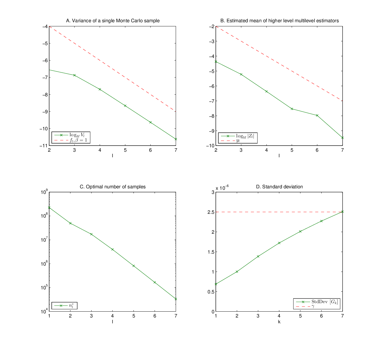
The results in Fig. 4 are presented in the same format as Fig. 3 earlier for the constant recovery rate. There is clear evidence that the convergence of the variance and mean are still both of first order in , where is the basket size.
Another extension, also proposed in [2], are random factor loadings of the type
| (7.7) |
where is a given deterministic function and . This model can capture contagion effects where, for decreasing , firm values are more closely correlated to the common market factor in bad times. Such an extension fits directly in the general framework developed earlier in this paper, assuming the technical conditions on the cumulative density hold where needed (see in particular Theorem 2.2).
Outlook
We would expect there to be scope to apply the presented nested simulation approach to a wider range of settings beyond the particular application studied here. An interesting extension would be to the model from [9], where the analysis requires further tools accounting especially for the heterogeneity of the basket, resulting in non-exchangeability. While our motivation comes from credit baskets and some of the later results are specific to piecewise linear functionals encountered in the valuation of basket credit derivatives, we hope there to be a wider relevance of the main approach to the simulation of certain functionals arising in large interacting particle systems and elsewhere.
Acknowledgement: We thank Mike Giles for suggesting the improved estimator, and two anonymous referees for their helpful suggestions which improved the presentation of the results.
References
- [1] E.I. Altman, B. Brady, A. Resti, and A. Sironi, The Link between Default and Recovery Rates: Theory, Empirical Evidence, and Implications, J. Business, 78 (6), 2203–2208, November 2005.
- [2] L. Andersen and J. Sidenius, Extensions to the Gaussian copula: random recovery and random factor loadings , J. Credit Risk, 1 (1), 29–70, Winter 2004/05.
- [3] D. Belomestny, J. Schoenmakers, and F. Dickmann, Multilevel dual approach for pricing American style derivatives, Finance Stoch., DOI 10.1007/s00780-013-0208-5, 2013.
- [4] K. Bujok and C. Reisinger, Numerical valuation of basket credit derivatives in structural jump-diffusion models, J. Comp. Fin., 15(4), 115–158, 2012.
- [5] N. Bush, B. Hambly, L. Jin, H. Haworth, and C. Reisinger, Stochastic evolution equations in portfolio credit modelling, SIAM J. Finan. Math., 2, 627–664, 2011.
- [6] N. Chen, P. Glynn, and Y. Liu, Computing functions of conditional expectation via multilevel nested simulation, Conference Presentation at MCQMC 2012.
- [7] A. Dembo, J.-D. Deuschel, and D. Duffie, Large portfolio losses, Finance Stoch., 8, 3–16, 2004
- [8] A. Dembo and O. Zeitouni, Large deviations techniques and applications, Jones and Bartlett Pulishers, Boston, first edition, 1993.
- [9] K. Giesecke, K. Spiliopoulos, R.B. Sowers, and J.A. Sirignano, Large portfolio asymptotics for loss from default, Math. Finance, DOI 10.1111/mafi.12011, 2012.
- [10] O. Kallenberg, Probabilisitc symmetries and invariance principles, Springer, New York, 2005.
- [11] M. Giles, Multi-level Monte Carlo path simulation, Oper. Res., 56, 607–617, 2008.
- [12] P. Glasserman, W. Kang, and P. Shahabuddin, Large deviations in multifactor portfolio credit risk, Math. Finance, 17(3), 345–379, 2007.
- [13] A. Lipton, Assets with jumps, RISK, 15(9), 149–153, 2002.
- [14] O. Vasicek, Limiting loan loss probability distribution, KMV Corporation, Document Number: 9990000046, 1991.
Appendix A Moment computations
Proof.
[of Lemma 5.2] We begin by showing (5.4) and then deduce (5.5) and (5.6). We have
where
Hence, we get
As is -measurable and the are independent and identically distributed given with , we have
Using the fact that we have the required bound in (5.4).