Fast Wiener filtering of CMB maps
Abstract:
We present the application of a new method to compute the Wiener filter solution of large and complex data sets. Contrary to the iterative solvers usually employed in signal processing, our algorithm does not require the use of preconditioners to be computationally efficient. The new scheme is conceptually very simple and therefore easy to implement, numerically absolutely stable, and guaranteed to converge. We introduce a messenger field to mediate between the different preferred bases in which signal and noise properties can be specified most conveniently, and rephrase the signal reconstruction problem in terms of this auxiliary variable. We demonstrate the capabilities of the algorithm by applying it to cosmic microwave background (CMB) radiation data obtained by the WMAP satellite.
September 19-21, 2012
Laboratoire Astroparticule et Cosmologie, 10 rue A. Domon et L. Duquet, 75205 Paris 13, France
1 Introduction
Among the linear filters that make use of statistical information about the data, the generalized Wiener filter stands out as the maximum a posteriori solution for the case that signal and noise both follow a Gaussian distribution (Wiener 1949). Although Wiener filtering is of fundamental importance, only recently efficient algorithms have been developed for the relaxed assumption that the signal covariance is not known in advance (Wandelt et al. 2004; Enßlin & Frommert 2011, e.g.,).
Assuming a linear model for the observed data as a combination of signal and noise ,
| (1) |
the Wiener filter is defined as the solution of the equation
| (2) |
It plays an important role in signal processing. Taking the example of cosmic microwave background (CMB) radiation data, it is calculated during optimal power spectrum estimation (Tegmark 1997b; Bond et al. 1998; Oh et al. 1999; Elsner & Wandelt 2012b, e.g.,), likelihood analysis (Hinshaw et al. 2007; Dunkley et al. 2009; Elsner & Wandelt 2012c, e.g.,), mapmaking (Tegmark et al. 1997; Tegmark 1997a, e.g.,), and lensing reconstructions (Hirata et al. 2004; Smith et al. 2007, e.g.,), etc.
To evaluate Eq. (2) in practice can turn out very challenging for the large and complex data sets obtained by state of the art experiments. Problems occur as the size of and increase with the second power of the number of data samples, rendering the storage and processing of dense systems impractical. Fortunately, it is often feasible to specify sets of bases where signal and noise covariance become sparse. However, these bases are generally incompatible, i.e., it is not possible to represent them in a single basis as sparse systems such that Eq. (2) can be solved trivially. Numerical algorithms for the exact solution of the Wiener filter equation are therefore often complex, e.g., involving conjugate gradient solvers with multigrid preconditioners (Smith et al. 2007). Finding fast preconditioners that work is a highly non-trivial art, especially since the matrices of interest are often extremely ill-conditioned ().
In Sect. 2, we briefly describe a new iterative algorithm for the solution of the exact Wiener filter equation. We illustrate the approach by applying it to WMAP7 data in Sect. 3. Summarizing the main aspects of our findings, we then discuss possible extensions and areas of applications (Sect. 4). Details on the mathematical aspects of the method can be found in Elsner & Wandelt (2013).
2 Method
To efficiently compute the Wiener filter, we first introduce a messenger field with covariance . The covariance properties of this auxiliary variable are very simple: is proportional to the identity matrix, a property that is preserved under any orthogonal basis change. Therefore, while it may not be possible to directly apply expressions like to a data vector, we can always do so with combinations as and , no matter what basis is chosen to render and sparse.
To benefit from this possibility, we now specify equations for the signal reconstruction and the auxiliary field ,
| (3) | ||||
| (4) |
where we defined and introduced one additional scalar parameter , which we will use to accelerate convergence. We specify the covariance matrix of the auxiliary field according to . In the limit , the system of equations defined above reduces to the Wiener filter equation.
An outline of the algorithm can be given as follows. Initially, the vectors and are set to zero. We solve Eq. (3) for the auxiliary field in the basis defined by the noise covariance matrix. Next, we change the basis to, e.g., Fourier space, where can be represented easily. Then, we solve for using Eq. (4) given the latest realization of , and finally transform the result back to the original basis. It can be shown that the signal reconstruction converges exponentially and unconditionally to the Wiener filter solution (Elsner & Wandelt 2013). Based on a comparison to more standard conjugate gradient solvers, we find the final map to be accurate to about 1 part in , depending on the adopted stopping criterion.
3 WMAP analysis
We now demonstrate the application of the algorithm to the V-band data of the Wilkinson microwave anisotropy probe (Jarosik et al. 2011, WMAP711 1 Available from http://lambda.gsfc.nasa.gov,). We adopted the official WMAP extended temperature and polarization masks, reducing the sky fraction to around 70 %.
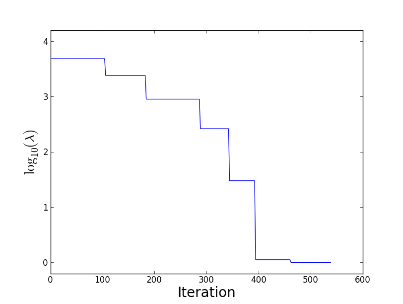
For the best performance in terms of computing time, we changed in the following way: To initialize the algorithm, we chose it according to the ratio at . As shown in Fig. 1, a high value of corresponds to a large convolution kernel in Eq. (4). Accordingly, small scales are smoothed out and information is more efficiently propagated into the masked regions. To monitor convergence of the algorithm, we used the of the current solution . After it has reached a plateau, we decreased to the ratio at . The evolution of , together with the current value of at every iteration, is depicted in Fig. 2. We stopped the algorithm as soon as the quality of the signal reconstruction improved only marginally between iterations, at , and obtain a final goodness of fit of .
Since we can attribute a specific length scale to a given value of (the current value of ), and fluctuations on smaller scales are suppressed owing to the width of the convolution kernel, we can restrict the maximum multipole moment of the computationally expensive spherical harmonic transforms to . As a result, the overall computing time for the spherical harmonic transforms can be reduced by a large margin. We note that for the most expensive final iterations, where and more than half of the computing time is spent, the algorithm is an excellent candidate for further acceleration by means of graphics processing units (Elsner & Wandelt 2011).
The buildup of the WMAP temperature Wiener filtered map is shown in Fig. 3. Characteristic for Wiener filter solutions, large scale fluctuations extend well inside masked regions. In Fig. 4, we plot the power spectra of the reconstruction for temperature and polarization, and demonstrate that the Wiener filter maps can be augmented to constrained realizations, with the correct signal variances.




4 Conclusion
We have summarized a new method to efficiently calculate the Wiener filter solution of general data sets. As a sample application, we analyzed WMAP temperature and polarization maps.
The algorithm is not only simple to implement, but also robust. Even after including polarization data in the analysis, it maintains good performance, despite of the increase in the condition number of the covariance matrices. We consider this fact to be of particular importance as conjugate gradient solvers are likely to perform noticeably worse in this setup.
We finally note that the algorithm is also very flexible, and many possible extensions are still to be explored. For some problems, for example, it may be beneficial to solve for the noise vector instead of the signal, which is calculated indirectly from the result. The auxiliary field then becomes associated with the signal reconstruction instead of the noise. In certain situations, it may also prove useful to include more than one messenger field, for example if multiple observations (e.g., from different detectors) should be combined in a joint analysis. It also remains to be explored to what extent our method could be combined with conventional iterative schemes, for example to act as a smoother in a multigrid scheme to speed up convergence further.
References
- Bond et al. (1998) Bond, J. R., Jaffe, A. H., & Knox, L. 1998, Phys. Rev. D, 57, 2117
- Dunkley et al. (2009) Dunkley, J., Komatsu, E., Nolta, M. R., et al. 2009, ApJS, 180, 306
- Elsner & Wandelt (2011) Elsner, F. & Wandelt, B. D. 2011, A&A, 532, A35
- Elsner & Wandelt (2012b) Elsner, F. & Wandelt, B. D. 2012b, A&A, 540, L6
- Elsner & Wandelt (2012c) Elsner, F. & Wandelt, B. D. 2012c, A&A, 542, A60
- Elsner & Wandelt (2013) Elsner, F. & Wandelt, B. D. 2013, A&A, 549, A111
- Enßlin & Frommert (2011) Enßlin, T. A. & Frommert, M. 2011, Phys. Rev. D, 83, 105014
- Hinshaw et al. (2007) Hinshaw, G., Nolta, M. R., Bennett, C. L., et al. 2007, ApJS, 170, 288
- Hirata et al. (2004) Hirata, C. M., Padmanabhan, N., Seljak, U., Schlegel, D., & Brinkmann, J. 2004, Phys. Rev. D, 70, 103501
- Jarosik et al. (2011) Jarosik, N., Bennett, C. L., Dunkley, J., et al. 2011, ApJS, 192, 14
- Oh et al. (1999) Oh, S. P., Spergel, D. N., & Hinshaw, G. 1999, ApJ, 510, 551
- Smith et al. (2007) Smith, K. M., Zahn, O., & Doré, O. 2007, Phys. Rev. D, 76, 043510
- Tegmark (1997a) Tegmark, M. 1997a, ApJ, 480, L87+
- Tegmark (1997b) Tegmark, M. 1997b, Phys. Rev. D, 55, 5895
- Tegmark et al. (1997) Tegmark, M., de Oliveira-Costa, A., Devlin, M. J., et al. 1997, ApJ, 474, L77
- Wandelt et al. (2004) Wandelt, B. D., Larson, D. L., & Lakshminarayanan, A. 2004, Phys. Rev. D, 70, 083511
- Wiener (1949) Wiener, N. 1949, The Extrapolation, Interpolation and Smoothing of Stationary Time Series with engineering applications (New York: John Wiley & Sons, Inc.)