Surprisingly Rational:
Probability theory plus noise explains
biases in judgment.
Abstract
The systematic biases seen in people’s probability judgments are typically taken as evidence that people do not reason about probability using the rules of probability theory, but instead use heuristics which sometimes yield reasonable judgments and sometimes systematic biases. This view has had a major impact in economics, law, medicine, and other fields; indeed, the idea that people cannot reason with probabilities has become a widespread truism. We present a simple alternative to this view, where people reason about probability according to probability theory but are subject to random variation or noise in the reasoning process. In this account the effect of noise is cancelled for some probabilistic expressions: analysing data from two experiments we find that, for these expressions, people’s probability judgments are strikingly close to those required by probability theory. For other expressions this account produces systematic deviations in probability estimates. These deviations explain four reliable biases in human probabilistic reasoning (conservatism, subadditivity, conjunction and disjunction fallacies). These results suggest that people’s probability judgments embody the rules of probability theory, and that biases in those judgments are due to the effects of random noise.
Keywords. probability; rationality; random variation; heuristics; biases
1 Introduction
The capacity to reason with uncertain knowledge (that is, to reason with probabilities) is central to our ability to survive and prosper in “an ecology that is of essence only partly accessible to foresight” (Brunswik,, 1955). It is therefore reasonable to expect that humans, having prospered in such an ecology, would be able to reason about probabilities extremely well: any ancestors who could not reason effectively about probabilities would not survive long, and so the biological basis of their reasoning would be driven from the gene pool. Probability theory provides a calculus of chance describing how to make optimal predictions under uncertainty: taking the argument one step further, it is reasonable to expect that our probabilistic reasoning will follow the rules of probability theory.
The conventional view in current psychology is that this expectation is wrong. Instead, the dominant position is that
In making predictions and judgments under uncertainty, people do not appear to follow the calculus of chance or the statistical theory of prediction. Instead they rely on a limited number of heuristics which sometimes yield reasonable judgments and sometimes lead to severe and systematic errors (Tversky and Kahneman,, 1973, p. 237)
This conclusion is based on a series of systematic and reliable biases in people’s judgements of probability, many identified in the 1970s and 1980s by Tversky, Kahneman and colleagues. This heuristics and biases approach has reached a level of popularity rarely seen in psychology (with Kahneman recieving a Nobel Prize in part for his work in this area). The idea that people do not reason using probability theory but instead follow various heuristics has been presented both in review articles describing current psychological research (Gigerenzer and Gaissmaier,, 2011, Shafir and Leboeuf,, 2002), and in numerous popular science books summarising this research for the general public (Ariely,, 2009, Kahneman,, 2011, e.g.). This approach has had a major impact in economics (Camerer et al.,, 2003, Kahneman,, 2003), law (Korobkin and Ulen,, 2000, Sunstein,, 2000), medicine (Dawson and Arkes,, 1987, Eva and Norman,, 2005) and other fields (Williams,, 2010, Hicks and Kluemper,, 2011, Bondt and Thaler,, 2012, Richards,, 2012). Indeed the idea that people cannot reason with probabilities has become a widespread truism: for example, the Science Gallery in Dublin recently presented an exhibition on risk which it described as “enabling visitors to explore our inability to determine the probability of everything from a car crash to a coin toss” (The Irish Times, Thursday, 11 October 2012).
We have two main aims in this paper: to give evidence against the view that people reason about probabilities using heuristics, and to give evidence supporting the view that people reason in accordance with probability theory, with bias in people’s probability estimates being caused by random variation or noise in the reasoning process. We assume a simple model where people estimate the probability of some event by estimating the proportion of instances of in memory, but are subject to random errors in the recall of instances. While at first glance it may seem that these random errors will result in “nothing more than error variance centered around a normative response” (Shafir and Leboeuf,, 2002), in fact these random errors cause systematic deviations that push estimates for away from the correct value in a characteristic way. In our model these systematic deviations explain various biases frequently seen in people’s probabilistic reasoning: conservatism, subadditivity, the conjunction fallacy, and the disjunction fallacy. The general patterns of occurrence of these biases match the predictions of our simple model.
We use this simple model to construct probabilistic expressions that cancel the bias in estimates for one event against the bias in estimates for another. These expressions allow us to test the predictions of the heuristics view of probabilistic reasoning. One such expression involves estimates, for some events and , of the individual probabilities and and the conjunctive (‘and’) and disjunctive (‘or’) probabilities and . People’s estimates for all four of these probabilities are typically subject to various forms of bias. Our account, however, predicts that when combined in the expression
(where represents a person’s estimate for , their estimate for , and so on), then the various biases on the individual expressions will cancel out, and on average will equal in agreement with probability theory’s ‘addition law’ which requires that
| (1) |
Notice that the heuristics view assumes that people estimate probabilities using heuristics that in some cases yield reasonable judgments (that is, judgments in accordance with probability theory) but in other cases lead to systematic biases. To give evidence against the heuristics view it is therefore not enough to show that some of people’s probability judgments agree with probability theory (that is expected in the heuristics view). Instead, our evidence against the heuristics view consists of results showing that, even when people’s probability estimates for a set of events are systematically biased, when those estimates are combined to form expressions like , the results are on average strikingly close to those required by probability theory. This cancellation of bias is difficult to explain in the heuristics view: to explain this cancellation, the heuristics view would require some way of ensuring that, when applying heuristics to estimate the probabilities , , and individually, the biases produced in those probabilities are precisely calibrated to give overall cancellation. Further, to ‘know’ that the bias in these four probabilities should cancel out in this way requires access to the rules of probability theory (as embodied in the addition law in this case). Since the heuristics view by definition does not follow the rules of probability theory, it does not have access to these rules and so has no reason to produce this cancellation.
We also use this model to construct a series of expressions where all but one ‘unit’ of bias is cancelled; our model predicts that the level of bias when people’s responses are combined in these expressions should on average have the same constant value. Our experimental results confirm this prediction, showing the same level of bias across a range of such expressions. Together, these results demonstrate that when noise in recall is cancelled, people’s probability estimates follow the rules of probability theory and thus suggest that biases in those estimates are due to noise. These results are the main contribution of our work.
Note that our evidence against the view that people use heuristics to estimate probabilities is not based on the fact that our model explains the four biases mentioned above (there are many other biases in the literature which our model does not address; see Hilbert, (2012) for a review). Instead, the point is that our experimental results show that the basic idea behind the heuristics view (that people do not follow the rules of probability theory) is contradicted when we use our simple model to cancel the effects of noise.
1.1 Bayesian models of reasoning
We are not alone in arguing that people reason in accordance with probability theory. Though “the bulk of the literature on adult human reasoning” goes against this view (Cesana-Arlotti et al.,, 2012), in recent years various groups of researchers have suggested that people follow mathematical models of reasoning based on Bayesian inference, a process for drawing conclusions given observed data in a way that follows probability theory. Bayesian inference applies to conditional probabilities such as the probability of some conclusion given some evidence : . In Bayesian models these conditional probabilities are computed according to Bayes’ theorem
and so the value of the conditional probability depends on the value of the ‘prior’ (the probability of being true independent of the evidence ) and on the value of the ‘likelihood function’ (the probability of seeing evidence given that the hypothesis is true).
The status of these Bayesian models is currently controversial. On one hand, close fits between human responses and Bayesian models have been demonstrated in domains as diverse as categorisation, naive physics, word learning, vision, logical inference, motor control and conditioning (Tenenbaum et al.,, 2011, Chater et al.,, 2006, Oaksford and Chater,, 2007, see e.g.), leading researchers to conclude that “everyday cognitive judgements follow [the] optimal statistical principles” of probability theory (Griffiths and Tenenbaum,, 2006). On the other hand, critics have pointed out a range of problems with this Bayesian approach (Bowers and Davis,, 2012, Marcus and Davis,, 2013, Eberhardt and Danks,, 2011, Jones and Love,, 2011, Endress,, 2013). For example, the estimation of priors and likelihood functions in Bayesian models is problematic: there are “too many arbitrary ways that priors, likelihoods etc. can be altered in a Bayesian theory post hoc. This flexibility allows these models to account for almost any pattern of results” (Bowers and Davis,, 2012).
It is important to stress that our approach is not connected to this Bayesian view. Our model applies only to the estimation of ‘simple’ probabilities such as the probability of some event , and does not involve Bayes’ theorem or conditional probabilities of any form. Neither does our model involve parameter estimation, priors, or likelihood functions. Equally, our results showing that people’s probability estimates follow the requirements of probability theory when noise is cancelled do not imply that people follow Bayes’ theorem when estimating conditional probabilities: Bayes’ theorem is significantly more complex than the simple probabilities we consider.
1.2 Overview
In the first section of the paper we present our model and show how it can explain the observed biases of conservatism, subadditivity, the conjunction fallacy, and the disjunction fallacy. In this section we also discuss other accounts for these biases, some of which are also based on noise (Costello, 2009a, , Costello, 2009b, , Erev et al.,, 1994, Hilbert,, 2012, Nilsson et al.,, 2009, Juslin et al.,, 2009, Dougherty et al.,, 1999, see). The crucial difference between our account and others is that our account makes specific and testable predictions about the degree of bias in probabilistic expressions, and about expressions where that bias will vanish. In the second and third sections we present our model’s predictions and describe two experimental studies testing and confirming these predictions. In the final sections we give a general discussion of our work.
2 Probability estimation with noisy recall
We assume a rational reasoner with a long-term episodic memory that is subject to random variation or error in recall, and take to represent a reasoner’s estimate of the probability of event . We assume that long-term memory contains episodes where each recorded episode holds a flag that is set to if contains event and set to otherwise, and the reasoner estimates the probability of event by counting these flags.
We assume a minimal form of transient random noise, in which there is some small probability that when some flag is read, the value obtained is not the correct value for that flag. We assume that this noise is symmetric, so that the probability of being read as is the same as the probability of being read as . We also assume a minimal representation where every type of event, be it a simple event , a conjunctive event , a disjunctive event , or any other more complex form, is represented by such a flag, and where every flag has the same probability of being read incorrectly. (We stress here that this type of sampling error is only one of many possible sources of noise. While we use this simple form of sampling error to motivate and present our model, our intention is to demonstrate the role of noise – from whatever source – in causing systematic biases in probability estimates.)
We take to be the number of flags marking that were read as in some particular query of memory, and be the number of flags whose correct value is actually . Our reasoner computes an estimate by querying episodic memory to count all episodes containing and dividing by the total number of episodes, giving
| (2) |
Random error in recall (and hence in the value of ) means that varies randomly: sampling repeatedly will produce a series of different values, varying due to error in recall. We assume that this estimation process is the same for every form of event: a probability estimate for a simple event is computed from the number of flags marking that were read as in some particular query of memory, a probability estimate for a conjunctive event is computed from number of flags marking that were read as in some particular query of memory, and so on.
We take to represent the ‘true’ judgment of the probability of : the estimate that would be given if the reasoner that was not subject to random error in recall and produced estimates in a perfect, error-free manner. We take to represent the expected value or population mean for . This is the value we would expect to obtain if we averaged an infinite number these randomly varying estimates . Finally, we take to represent a sample mean: the average of some finite set of estimates . This sample mean will vary randomly around the population mean , with the degree of random variation in the sample mean decreasing as the size of the sample increases.
For any event the expected value of is given by
(since on average of the flags whose value is will be read as , and of the flags whose value is will be read as ). Since by definition
we have
| (3) |
and the expected value of deviates from in a way that systematically depends on .
Individual estimates will vary randomly around this expected value and so for any specific estimate where flags were read as having a value of , we have
| (4) |
where
represents positive or negative random deviation from the expected value across all estimates. Note that this error term does not introduce an additional source of random error in probability estimates: it simply reflects the difference between the number of flags that were read incorrectly when computing the specific estimate and the the number of flags that are read incorrectly on average, across all estimates.
Finally, we can also derive an expression for the expected variance in these randomly varying estimates . The expected variance is equal to for all events , , and so on, and is independent of event probability; see the Appendix for details.
2.1 Conservatism
In this section we show how our noisy recall model of probabilistic reasoning explains a reliable pattern of conservatism seen in people’s probability estimates.
Probabilities range in value between and . A large body of literature demonstrates that people tend to keep away from these extremes in their probability judgments, and so are ‘conservative’ in their probability assessments. These results show that the closer is to , the more likely it is that is greater than , while the closer is to , the more likely it is that is less than . Differences between true and estimated probabilities are low when is close to and increase as approaches the boundaries of or . This pattern was originally seen in research on people’s revision of their probablity estimates in the light of further data (Edwards,, 1968), and was later found directly in probability estimation tasks. This pattern is sometimes referred to as underconfidence in people’s probability estimates (see Erev et al.,, 1994, Hilbert,, 2012, for a review).
Conservatism will occur as a straightforward consequence of random variation in our model. As we saw in Equation 3, the expected value of deviates from in a way that systematically depends on . If this deviation will be . If then since cannot be negative we have , with the difference increasing as approaches . Since estimates are distributed around this means that will tend to be greater than , with the tendency increasing as approaches . Similarly if then and estimates will tend to be less than , with the tendency increasing as approaches . This deviation thus matches the pattern of conservatism seen in people probability judgments.
2.1.1 Other accounts
The idea that conservatism can be explained via random noise is not new to our account, but is also found in Erev et al., (1994)’s account based on random error in probability estimates, in the Minerva-DM memory-retrieval model of decision making (Dougherty et al.,, 1999), and in Hilbert’s account based on noise in the information channels used in probabilistic reasoning (Hilbert,, 2012). The underlying idea in these accounts is similar to ours. There is, however, a critical difference: our account predicts no systematic bias for probabilistic expressions with a certain form (see Section ).
2.2 Subadditivity
Here we show how our noisy recall model explains various patterns of ‘subadditivity’ seen in people’s probability estimates.
Let be a set of mutually exclusive events, and let be the disjunction (the ‘or’) of those events. Then probability theory requires that
Experimental results show that people reliably violate this requirement, and in a characteristic way. On average the sum of people’s probability estimates for events is reliably greater than their estimate for the probability of , with the difference (the degree of subadditivity) increases reliably as increases. An additional, more specific pattern is also seen: for pairs of mutually exclusive events and whose probabilities sum to we find that the sums of people’s estimates for and are normally distributed around , and so on average this sum is equal to just as required by probability theory. This pattern is sometimes referred to as ‘binary complementarity’ (see Tversky and Koehler,, 1994, for a detailed review of these results).
Again, these patterns of subadditivity occur as a straightforward consequence of random variation in our model. From Equation 3 we have
and using the fact that this gives
Taking the difference between this expression and that for in equation 3 we get
and so this difference increases as increases, producing subadditivity as seen in people’s probability judgments. In the case of two mutually exclusive events and whose probabilities sum to , from Equation 3 we get
producing binary complementarity as seen in people’s judgments.
2.2.1 Other accounts
The original account for subadditivity given by Tversky and Koehler, (1994) explained the general pattern in terms of an unpacking process which increased the probability of constituent events by drawing attention to their components. This account could not explain the observed pattern of binary complementarity; to account for this observation Tversky and Keohler proposed an additional ‘binary complementarity’ heuristic, which simply stated that there was no average bias for binary complements.
An alternative explanation for subaddivity is given in the Minerva-DM memory retrieval model of decision making(Dougherty et al.,, 1999, Bearden and Wallsten,, 2004). Minerva-DM is a complex model with a number of different components: it provides a two-step process for conditional probability judgments, a parameter controlling the retrieval of items with varying degrees of similarity to the memory probe (the event whose probability is being judged), a complex multi-vector representation for stored items in memory, a parameter controlling the degree of random error in the initial recording of items in memory, a parameter controlling the degree of random error causing degradation in stored items, and a parameter controlling the degree of detail contained in memory probes. Roughly stated, the Minerva-DM model estimates the probability of some event by counting the number of stored items in memory which are similar enough to that event (whose similarity measure is greater than the similarity criterion parameter). Depending on the value of the similarity criterion, this count will include a number of similar-but-irrelevant items in addition to items correctly matching the target event. Because of these similar-but-irrelevant items, the model will give a probability estimate for the target event that is higher than the true probability, producing a degree of subaddivity that increases with the number of component events in the disjunction, just as required. Note, however, that because this similarity-based account always increases probability estimates, it cannot explain the observed pattern of binary complementarity in people’s probability judgments, which can only be explained if one probability is increased and the other complementary probability is decreased.
More recently, Hilbert, (2012) gave an account of subadditivity based on noise in the information channels used for probability computation. Hilbert’s model is a very general one, providing for noise at the initial encoding of data, for noisy degradation of stored information and for noise during the reading of data from memory. The model also specifies three general requirements for the distribution of noise: that the correct probability is most likely, that noise is symmetrical around the correct probability and that two binary complementary probabilities have the same degree of noise. The last of these requirements allows the model to explain the ‘binary complementarity’ result observed by Tversky and Koehler, (1994). Beyond these requirements, the model leaves the degree and form of noise in the system unspecified. Again, this account is similar to ours but with the crucial difference that our account predicts no systematic bias for certain probabilistic expressions. We give a further comparison between our model, Hilbert’s model and Minerva-DM in Section .
2.3 Conjunction and disjunction fallacies
Conservatism and subadditivity both concern averages of people’s probability estimates. Here we show how our noisy recall model explains two patterns that involve differences between individual probability estimates: the conjunction and disjunction fallacies.
Let and be any two events ordered so that . Then probability theory’s ‘conjunction rule’ requires that ; this follows from the fact that can only occur if itself occurs. People reliably violate this requirement for some events, and commit the ‘conjunction fallacy’ by giving probability estimates for conjunctions that are greater than the estimates they gave for one or other constituent of that conjunction. Perhaps the best-known example of this violation comes from Tversky & Kahneman (1983) and concerns Linda:
“Linda is 31 years old, single, outspoken, and very bright. She majored in philosophy. As a student she was deeply concerned with issues of discrimination and social justice, and also participated in anti-nuclear demonstrations”
Participants in Tversky & Kahneman’s study read this description and were asked to rank various statements “by their probability”. Two of these statements were
Linda is a bank teller. ()
Linda is a bank teller and active in the feminist movement.()
In Tversky & Kahneman’s initial investigation these two statements were presented separately, with one group of participants ranking a set of statements containing but not , and a second group ranking the same set but with replaced by . The results showed that the average ranking given to by the second group was significantly higher than the average ranking given to by the first group, violating the conjunction rule.
Note that violation of the conjunction rule can occur in averaged data even when very few participants are individually committing the conjunction fallacy; equally, this violation is not necessarily seen in averaged data even when many participants are individually committing that fallacy. For this reason, Tversky & Kahneman refer to this comparison of averages as an ‘indirect’ test of the conjunction rule, and describe violations of that rule in averages as conjunction errors. Surprised by the results of their indirect test, Tversky & Kahneman carried out a series of increasingly direct tests of the conjunction rule. In these direct tests each participant were asked to rank the probability of a set of statements containing both and . Tversky & Kahneman found that in some cases more than of participants ranked as more probable than , violating the conjunction rule in their individual responses. Tversky & Kahneman use the term ‘conjunction fallacy’ to refer only to these direct violations of the conjunction rule. Most subsequent studies have focused on similar direct tests of the conjunction rule in individual probability estimates (the conjunction fallacy) rather than on indirect tests comparing averages (the conjunction error).
The Linda example is explicitly designed to produce the conjunction fallacy: this fallacy does not occur for all or even most conjunctions. Numerous experimental studies have shown that the occurrence of this fallacy depends on the probabilities of and . In particular, the greater the difference between and , the more frequent the conjunction fallacy is, and the greater the conditional probability , the more frequent the conjunction fallacy is (Costello, 2009a, , Gavanski and Roskos-Ewoldsen,, 1991, Fantino et al.,, 1997).
A similar pattern occurs for people’s probability estimates for disjunctions . Since necessarily occurs if itself occurs, probability theory requires that must always hold. People reliably violate this requirement for some events, giving probability estimates for disjunctions that are less than the estimates they gave for just one of the constituents. Just as for conjunctions, the greater the difference between and , and the higher the estimated conditional probability , the higher the rate of occurrence of the disjunction fallacy (Costello, 2009b, , Carlson and Yates,, 1989).
The observed patterns of conjunction and disjunction fallacy occurrence arise as a straightforward consequence of random variation in our model. The general idea is that our reasoner’s probability estimates and will both vary randomly around their expected values and . This means that, even though must hold, there is a chance that the estimate for will be greater than the estimate for , producing a conjunction fallacy. This chance will increase the closer is to .
More formally, the reasoner’s estimates for probabilites and at any given moment are given by
| and |
where and represent positive or negative random deviation from the expected estimate at that time (arising due to random errors in reading flag values from memory, as in Equation 4). The conjunction fallacy will occur when , i.e. when
or, substituting and rearranging, when
| (5) |
holds. Given that and vary randomly and can be either positive or negative, this inequality can hold in some cases. The inequality is most likely to hold when is low (because in that situation the left side of the inequality is low). Since , we see that is low when is low and both and are high (or more strictly: when is close to , is close to , and is close to its maximum possible value of ). We thus expect the conjunction fallacy to be most frequent when is low and and are both high. This is just the pattern seen when the conjunction fallacy occurs in people’s probability estimates.
Reasoning in just the same way for disjunctions, we see that the disjunction fallacy will occur when
or, substituting and rearranging as before, when
holds. But from probability theory, we have the identity
and substituting we see that the disjunction fallacy will occur when
| (6) |
and so, just as with the conjunction fallacy, we expect the disjunction fallacy to be most frequent when is low and and are both high. Again, this is just the pattern seen when the disjunction fallacy occurs in people’s probability estimates.
Note that in our model there is an upper limit on the expected rate of conjunction fallacy occurrence of , which occurs when : estimates and are distributed around the same population means, and so the chance of getting is the same as the chance of getting . The same limit holds for the disjunction fallacy, and for the same reason. This limit occurs because our simple model assumes (somewhat unrealistically) that the degree of error in recall for examples of is the same as the degree of error in recall for for (extensions of our model which allow for different levels of error in recall for and would not impose this limit). As we see in the next section, however, experiments which control for various extraneous factors typically give conjunction fallacy rates which are consistent with this limit.
2.4 The reality of the conjunction fallacy
A number of researchers have attempted to ‘explain away’ the conjunction fallacy by pointing to possible flaws in Tversky & Kahneman’s Linda experiment which may have led participants to give incorrect responses. One argument in this line is to propose that the fallacy arises because participants in the experiments understand the word ‘probability’ or the word ‘and’ in a way different from that assumed by the experimenters. A related tactic is to propose that the fallacy occurs because participants, correctly following the pragmatics of communication in their experimental task, interpret the single statement as meaning ( and not ). Evidence against these proposals comes from experiments using a betting paradigm, where the word ‘probability’ is not mentioned and where ‘and’ is demonstrably understood as meaning conjunction, and experiments where participants are asked to choose among three different options , and . Conjunction fallacy rates are typically reduced in these experiments (to between and , as compared to the greater than rate seen in Tversky & Kahneman’s Linda experiment), but remain reliable (Sides et al., 2002a, , Tentori et al., 2004a, , Wedell and Moro,, 2008, see, for example,).
Another approach is to explain away the conjunction fallacy by arguing that Tversky & Kahneman’s probabilistic ranking task is not in a form that is suitable for people’s probabilistic reasoning mechanisms, which (in this argument) are based on representations of frequency. The suggestion is that if participants were asked to estimate the frequency with which constituent and conjunctive statements are true, the conjunction fallacy should vanish (Hertwig and Gigerenzer,, 1999). In the Linda task, this frequency format could involve giving participants a story about a number of women who fit the description of Linda, then asking them to estimate ‘how many of these women are bank tellers’ and ‘how many of these women are bank tellers and are active in the feminist movement’. However, studies have repeatedly shown that while the occurrence of the conjunction fallacy declines in frequency format tasks (typically going from a rate greater than in Linda tasks to a rate between and in frequency format tasks) the fallacy remains reliable and does not disappear (Mellers et al.,, 2001, Fiedler,, 1988, Chase,, 1998). Indeed, Tversky & Kahneman’s original 1983 paper examined the role of frequency formulations in the conjunction fallacy, and found that the fallacy was reduced but not eliminated by that formulation.11 1 Note, however, that conjunction errors (that is, violations of the conjunction rule in indirect tests on averages rather than in direct tests on individual responses) can be eliminated by this frequency formulation (Mellers et al.,, 2001). Taken together, these results suggest that the conjunction fallacy rates of and above found by Tversky & Kahneman are artifically high because of various confounding factors: studies of the conjunction fallacy that eliminate these factors give fallacy rates that are generally around or lower, in line with our model’s expectations.
2.4.1 Other accounts
A large and diverse range of accounts have been proposed for the conjunction and disjunction fallacies. Tversky & Kahneman’s original proposal explained these fallacies in terms of a representativeness heuristic, in which probability is assessed in terms of the degree to which an instance is representative of a (single or conjunctive) category. Under Tversky & Kahneman’s interpretation, in the Linda example people gave a higher rating to the conjunctive statement because the instance Linda was more representative of (that is, more similar to members of) the conjunctive category ‘bank-teller and active-feminist’ than the single category ‘bank-teller’.
Although the representativeness heuristic remains the routine explanation of the conjunction fallacy in introductory textbooks, a number of experimental results give convincing evidence against this account. Notice that the representativeness heuristic only applies when a question asks about the probability of membership of an instance in a conjunctive category, and only applies when knowledge about representative members of that category is available. Evidence against representativeness comes from results showing that the conjunction fallacy occurs frequently when these requirements do not hold. For example, a series of studies by Osherson, Bonini and colleagues have shown that the conjunction fallacy occurs frequently when people are asked to bet on the occurrence of unique future events: such bets are not questions about membership of an instance in a category, and so representativeness cannot explain the occurrence of the fallacy in these cases (Sides et al., 2002b, , Tentori et al., 2004b, , Bonini et al.,, 2004). Gavanski and Roskos-Ewoldsen, (1991) found that the conjunction fallacy occurred frequently when people are asked about categories for which no representativeness information is available (questions about imaginary aliens on other planets). Gavanski and Roskos-Ewoldsen, (1991) also found that the fallacy occurred frequently when the probability question was not about the membership of an instance in a conjunctive category, but about the membership of two separate instances in two separate single categories (rather than asking about the probability of Linda being a bank teller and active feminist, such questions might ask about the probability of Bob being a bank teller and Linda being an active feminist). Again, representativeness cannot explain the occurrence of the conjunction fallacy for such questions (see Nilsson et al.,, 2009, for a review of research in this area).
The Minerva-DM account gives an alternative explanation for the conjunction fallacy that is based on the role of similarity in retrieval (Dougherty et al.,, 1999). Minerva-DM estimates the probability of some event by counting the number of stored items in memory whose similarity to the probe event is greater than the similarity criterion parameter. For a conjunction , stored items that are members of alone or members of alone can be similar enough to the conjunction to be (mistakenly) counted as examples of that conjunction. If there are a large number of such similar-but-irrelevant items, the conjunctive probability estimate may be higher than the lower constituent probability , producing a conjunction fallacy response. Note, however, that because this similarity-based account always increases probability estimates, it cannot explain the disjunction fallacy (which occurs when a disjunctive probability estimate is lower than one of its constituent probabilities).
Other accounts have been proposed where people compute conjunctive probabilities from consituent probabilities and using some equation other than the standard equation of probability theory. In early versions of this approach the conjunctive probability was taken to be the average of the two constituent probabilities (Fantino et al.,, 1997, Carlson and Yates,, 1989). This averaging approach does not apply to disjunctive probabilities. More recently Nilsson, Juslin and colleagues (Nilsson et al.,, 2009, Juslin et al.,, 2009) have proposed a more sophisticated ‘configural cue’ model where conjunctive probabilities are computed by a weighted average of constituent probability values, with a greater weight given to the lower constituent probability, and where disjunctive probabilities are computed by a weighted average with greater weight given to the higher constituent probability.
Since the average of two numbers is always greater than the minimum of those two numbers and less than the maximum (except when the numbers are equal), these averaging accounts predict that the conjunction fallacy will occur for almost every conjunction (except when the two constituents have equal probabilities). This is clearly not the case, however: there are many conjunctions for which these fallacies occurs rarely if at all. To address this problem, Nilsson et al.’s model also includes a noise component which randomly perturbs conjunctive probability estimates, sometimes moving the conjunctive probability below the lower constituent probability and so eliminating the conjunction fallacy for that estimate. This model thus predicts that fallacy rates should be inversely related to the degree of random variation in people’s probability judgments, with fallacy rates being highest when random variation is low and lowest when random variation is high. This contrasts with our account, which predicts that fallacy rates should be high when random variation is high and low when random variation is low. We assess these competing predictions in Section 4.3.
Finally, we should mention an earlier model for the conjunction fallacy proposed by one of the authors (Costello, 2009a, ). Just as in our current account, this earlier model proposed that people’s probability estimates followed probability theory but were subject to random variation: this random variation caused conjunction fallacy responses to occur when constituent and conjunctive probability estimates were close together. Apart from that commonality, the two models are quite different. Unlike our current account, this earlier model was not based on the idea of noise causing random errors in retrieval from memory: instead, that model assumed that estimates for some event were normally distributed around the correct value , and so the average estimate was equal to the true value . That earlier model was therefore unable to account for the patterns of conservatism and subadditivity seen in people’s probability estimates. Also unlike our current account, that earlier model assumed that conjunctive and disjunctive probabilities were computed by applying the equations of probablity theory to constituent probability estimates, so that . This contrasts with the current model, which computes by retrieving episodes of the event from memory.
3 Experiment 1
Our noisy recall model of probability estimation can explain various patterns of bias in people’s probability judgements, and also explain some specific situations in which those biases vanish (when probabilities are close to , for conservatism; and when two complementary probabilities sum to , for subadditivity). We now present a third situation in which our model predicts that bias will disappear.
Consider an experiment where we ask people to estimate, for any pair of events and , the probabilities of , , and . For each participant’s estimates for each pair of events and , we can compute a derived sum
We can make a specific prediction about the expected value of for all events and : this value will be
From Equation 3 we get
However, probability theory requires for all events and , and so . Our prediction, therefore, is that the average value of across all pairs of events and will be equal to . Note that this prediction is invariant: it holds for all pairs of events and , irrespective of the degree of co-occurrence or dependency between those events.
What is the distribution of values of around this average of ? Speaking generally, we would expect this distribution to be unimodal and roughly symmetric around the mean of for any pair , since the positive and negative terms in the expression are symmetric: .
We examined this expectation in detail via Monte Carlo simulation, by writing a program that simulates the effects of random noise in recall on probability estimations for a given set of probabilities. This program took as input three probabilities , and ( and ). The program constructed a ‘memory’ containing items, each item containing flags , , and indicating whether that item was an example of the given event. The occurrence of those flags in memory exactly matched the probabilities of the given event as specified by the three input probabilities (so the occurrence of , for example, matched the sum of input probabilities and ). This program also contained a noise parameter (set to in our simulations); when reading flag values from memory to generate some probability estimate , the program was designed to have a random chance of returning the incorrect value.
We carried out this simulation process for a representative set of values for the input probabilities , and . These set consisted of every possible assignment of values from to each input probability, subject to the requirement that both and must both hold. This requirement ensures that every set of input probabilities was consistent with the rules of probability theory. In total there were sets of input probabilities that were consistent with these requirements. For each such set of input probabilities the program carried out runs, on each run generating noisy estimates , , and and using those estimates to calculate a value for the expression . These runs give us a picture of the distribution of values of .
The distribution of values was essentially the same for all these sets of input probabilities: unimodal, approximately symmetric, and centered on , just as expected. Figure 1 graphs the frequency distributions of all values across all probability sets. Given that this distribution appears to be essentially independent of the probability values used in our simulations, our prediction is that in an experiment, the distribution of across all pairs of events and will be unimodal and approximately symmetric around the mean of .
One possible concern with this simulation comes from the common observation that, when estimating probabilities, participants tend to respond in units that are multiples of or (Budescu et al.,, 1988, Wallsten et al.,, 1993, Erev et al.,, 1994). To test the impact of this rounding, we modified our simulation program to include a rounding parameter such that each calculated probability estimate was rounded to the nearest unit of . We ran the simulation as before but with set to , and , and examined the distribution of values for each run: the distribution was essentially the same as that shown in Figure 1, confirming our original simulation results.
3.1 Testing the predictions
We tested these predictions using data from an experiment on conjunction and disjunction fallacies (Costello, 2009b, , Experiment in). The original aim of this experiment was to examine an attempt by Gigerenzer to explain away the conjunction fallacy as a consquence of people being asked to judge the probability of one-off, unique events (Gigerenzer,, 1994). Gigerenzer argued that from a frequentist standpoint the rules of probability theory apply only to repeatable events and not to unique events, and so people’s deviation from the rules of probability theory for unique events are not, in fact, fallacious. To assess this argument, the experiment examined the occurrence of fallacies in probability judgements for conjunctions and disjunctions of canonical repeatedly-occurring events: weather events such as ‘rain’, ‘wind’ and so on. Contrary to Gigerenzer’s argument, participants in these experiments often committed conjunction and disjunction fallacies; these fallacies thus cannot be dismissed as an artifact of researchers using unique events in their studies of conjunctive probability.
This experiment gathered estimates , , and from participants for pairs of weather events. Two sets of weather events (the set ‘cloudy, windy, sunny, thundery’ and the set ‘cold, frosty, sleety’) were used to form these pairs. These sets were selected so that they contained events of high, medium and low probabilities. Conjunctive and disjunctive weather events were formed by pairing each member of the first set with every member of the second set and placing ‘and’/‘or’ between the elements as required, generating weather events such as ‘cloudy and cold’, ‘cloudy and frosty’, and so on. One group of participants () were asked questions in terms of probability, of the form
- •
What is the probability that the weather will be on a randomly-selected day in Ireland?
for some weather event . This weather event could be a single event such as ‘cloudy’, a conjunctive event such as ‘cloudy and cold’ or a disjunctive event such as ‘cloudy or cold’. The second group () were asked questions in terms of frequency, of the form
- •
Imagine a set of 100 different days, selected at random. On how many of those 100 days do you think the weather in Ireland would be ?
where the weather events were as before. These two question forms were used because of a range of previous work showing that frequency questions can reduce fallacies in people’s probability judgments; the aim was to check whether this question form could eliminate fallacy responses for everyday repeated events.
Participants were given questions containing all single events and all conjunctive and disjunctive events, with questions presented in random order on a web browser. Responses were on an integer scale from to . There was little difference in fallacy rates between the two forms of question, so we collapse the groups together in our analysis. There were distinct conjunction and disjunction responses in the experiment ( participants conjunctions): a conjunction fallacy was recorded in of those responses and a disjunction fallacy in .
For every pair of weather events used in the experiment, each participant gave estimates for the two constituents and , for the conjunction and for the disjunction . Each participant gave these estimates for such pairs. For each participant we can thus calculate the value for pairs , and so across all participants we have distinct values of . Our prediction is that the average of these values will equal and that these values will be approximately symmetrically distributed around this average.
3.2 Results
Figure 2 graphs the raw frequency of occurrence of values for in the experimental data and the average frequency in groups of those values. It is clear from the graph that these values are symmetrically distributed around the mean, just as expected. The mean value of was (SD=), within unit of the predicted mean on the -point scale used in the experiment and within standard deviations of the predicted mean. The predicted mean of lay within the confidence interval of the observed mean. This is in strikingly close agreement with our predictions. Note that the sequence of higher raw frequency values (hollow circles) in Figure 2 fall on units of , and represent participants’ preference for rounding to the nearest (the nearest unit of ) in their responses: approximately of all responses were rounded in this way.
To examine the relationship between conjunction and disjunction fallacy rates and values we compared the total number of conjunction and disjunction fallacies produced by each participant with the average value of for that participant. Figure 3 graphs this comparison. There was no significant correlation between the average value of produced by a participant and the number of fallacies produced by that participant (, ).
3.3 Discussion
The above result is based on a specific expression that cancels out the effect of noise in people’s probability judgements. When noise is cancelled in this way, we get a mean value for that is almost exactly equal to that predicted by probability theory. This close agreement with probability theory occurs alongside significant conjunction and disjunction fallacy rates in the same data, with values of close to zero even for participants with high conjunction and disjunction fallacy rates (Figure 3). This cancellation of bias is difficult to explain in the heuristics view: to explain this cancellation, the heuristics view would require some way of ensuring that, when using heuristics to estimate the probabilities , , and individually, the various biases in those estimates are calibrated to give overall cancellation. Note that from both the conservatism results and the binary complementarity results described earlier, we know that the bias in estimates and will tend to cancel only when (that is, when and are complementary). For the heuristics account to explain cancellation of bias across the terms in , therefore, it is not enough to say that people overestimate and underestimate : it is necessary to calibrate the varying degrees of bias affecting all probability estimates for , , and .
Further, to ‘know’ that the bias in these probabilities should cancel out in this way requires access to the rules of probability theory (as embodied in the addition law). These results therefore show that that people follow probability theory when judging probabilities, and that the observed patterns of bias are due to the systematic distorting influence of noise: when distortions due to noise are cancelled out as in expression , no other systematic bias remains.
In the next section we describe a new experiment re-testing this result and testing similar predictions for a range of other expressions.
4 Experiment 2
Our prediction for the derived expression holds because the associated expression is identically , and because there are an equal number of positive and negative terms in the expression (these two requirements are necessary to cancel out the or noise terms in the expression). We now give another expression where these requirements both hold, and so for which the same prediction follows.
Consider an experiment where we ask people to estimate, for any pair of events and , the probabilities of , , , , ( and not ) and ( and not ). One derived sum which involves these probabilities is
whose expected value will be
From Equation 3 we get
However, probability theory requires (because each side of the expression is equal to ) and so we have for all events and , and again we predict that the average value of across all participants and event pairs will equal to . Since the positive and negative terms in the expression are symmetric (just as in ), we again expect values for to be symmetrically distributed around this mean, just as with (this prediction is supported by Monte Carlo simulations similar to those described earlier). Finally, since both and have the same mean of , we predict that the larger combined set of all values of and across all participants and event pairs will also have an mean of , and will be symmetrically distributed around that mean.
We can also consider other derived sums whose values in probability theory are , but where there is not an equal number of positive and negative terms in the expression (and so not all or noise terms will be cancelled out). Four such expressions are
For the first expression , Equation 3 gives
since from probability theory for all and . We get the same result for the expressions , and , and so we have expected values of
for all pairs . Our prediction, therefore, is that expressions should all have the same average value in our experiment.
Two other such derived sums are
Similiar computations for these expressions tell us that will have an expected value of and will have an expected value for all pairs . Our prediction, therefore, is that expressions and should have the similar average values in our experiment, and that this average should be twice the average for . Note that since these expressions are not symmetric (all have ‘leftover’ terms) we do not expect the values of these expressions to be symmetrically distributed.
These last predictions are somewhat similar to the subadditivity results described earlier, in that both involve leftover terms. The subadditivity results only applied to disjunctions of exclusive events (events that did not co-occur). The current predictions are more general in that they hold for all pairs of events and , irrespective of the degree of co-occurrence or dependency between those events.
4.1 Method
Participants. Participants were undergraduate students at the School of Computer Science and Informatics, UCD, who volunteered for partial credit.
Stimuli. This experiment gathered people’s estimates for , , , , and for different pairs of weather events such as ‘rainy’,‘windy’ and so on. We constructed sets of three weather events each (the set ‘cold, rainy, icy’ and the set ‘windy, cloudy, sunny’), selected so that each set contained events of high, medium and low probabilities. Note that some of these pairs have positive dependencies (it is more likely to be rainy if it is cloudy), some had negative dependencies (it is less likely to be cold if it is sunny), and others were essentially independent: our predictions apply equally across all cases.
Conjunctive and disjunctive weather events were formed from these sets by pairing each member of the first set with every member of the second set and placing ‘and’/‘or’ between the elements as required, generating weather events such as ‘cold and windy’, ‘cold or cloudy’ and so on. Weather events describing conjunctions with negation were constructed by pairing each member of the first set with every member of the second set, taking the two possible orderings of the selected elements, and for each placing ‘and not’ between the elements in each ordering. This generated events such as ‘cold and not windy’ and ‘windy and not cold’ for each pair of events.
Procedure. Participants judged the probability of all single events and all conjunctions, disjunctions and conjunctions with negations. Questions were presented in random order on a web browser. One group of participants () were asked questions in terms of probability, of the form
- •
What is the probability that the weather will be on a randomly-selected day in Ireland?
for some weather event . This weather event could be a single event such as ‘cloudy’, a conjunctive event such as ‘cloudy and cold’, a disjunctive event such as ‘cloudy or cold’, or a conjunction and negation event such as ‘cloudy and not cold’ or ‘cold and not cloudy’. The second group () were asked questions in terms of frequency, of the form
- •
Imagine a set of 100 different days, selected at random. On how many of those 100 days do you think the weather in Ireland would be ?
where the weather events were as before. Responses were on an integer scale from to . The experiment took around minutes to complete.
4.2 Results
Two participants were excluded (one because they gave responses of to all but questions and the other because they gave responses of to all but questions), leaving participants in total. There were thus distinct conjunction and disjunction responses for analysis in the experiment ( participants conjunctions): a conjunction fallacy was recorded in of those responses and a disjunction fallacy in .
For every pair of weather events used in the experiment, each participant gave probability estimates for the two constituents and , for and , and for and . Each participant gave these estimates for nine such pairs. For each participant we calculated the value , and for nine pairs , and so across all participants we have distinct values for each of those expressions.
4.2.1 Expressions and
The mean value of was (SD=) and the mean value of was (SD=). Figure 4 graphs the raw frequency of occurrence of values of and in the experimental data and the average frequency in groups of those values, as in Figure 2. It is clear that these values are again unimodal and symmetrically distributed around their mean, as predicted. Averaging across all values of and we get a mean of (SD=); the predicted mean of lies with the confidence interval of this observed mean. (Again, the sequence of higher raw frequency values (hollow circles) in Figure 4 fall on units of , and represent participants’ preference for rounding to the nearest in their responses: approximately of all responses were rounded in this way.)
To examine the relationship between conjunction and disjunction fallacy rates and and values we compared the total number of conjunction and disjunction fallacies produced by each participant with the average and values for that participant. As in the previous experiment, there was no significant correlation between the average values produced by a participant and the number of fallacies produced by that participant ( and respectively); the results showed values of and close to zero even for participants with high conjunction and disjunction fallacy rates.
As before, these cancellation of bias results are difficult for the heuristics view to explain: they would require some way of ensuring that, when using heuristics to estimate the constituent probablities in , and the constituent probabilities in , the resulting biases are precisely calibrated to give overall cancellation. Further, to know that the bias in these probabilities should cancel requires access to the rules of probability theory, which the heuristics view does not have.
4.2.2 Expressions
Recall that in our model estimates for expressions should on average all have the same biased value, equal to (the noise rate). Table gives the average values for these expressions calculated from participant’s probability estimates; it is clear that these values are closely clustered (all are less than one tenth of an from the mean) just as predicted.
4.2.3 Expressions and
Recall that in our model estimates for expressions and should on average have the same biased value, equal to (twice the noise rate). Our prediction therefore is that values for and should fall close together, and should fall close to twice the overall mean obtained for expressions (as in Table ). Table gives the average values for these expressions calculated from participant’s probability estimates, and compares with twice the overall mean of . It is clear that these values are closely clustered around that predicted value (both are less than one-twentieth of an SD from the predicted value, and their mean is less than SD from that predicted value).
According to our model, the mean values of expressions are equal to the average value of , the rate of random error in recall from memory, and the mean values of expressions and are equal to twice that value. This raises the interesting possiblity of using the values of expressions for a given participant to estimate a value of for that participant, and so estimate the degree of variability due to noise in that participant’s probability estimates. We discuss this possibility in the next section.
4.3 Random variation and fallacy rates across participants
In our model the rate of occurrence of the conjunction fallacy is related to the degree of random variation: if there were no random variation in participant’s estimates the fallacy would never occur, while if there is a high degree of random variation the fallacy would occur frequently. The same prediction applies to the disjunction fallacy.
In this section we test these predictions using the data from our Experiment . In this analyis we use each participant’s average values for expressions to estimate a value of , the rate of random variation in recall for that participant. For each participant we can compute estimates for that participant’s value of , by taking that participant’s average value for each expression (and dividing the averages for and by ). To examine the consistency of these estimates, we computed the pairwise correlation across participants between values of estimated from each expression. Every pairwise correlation was significant at the level, and the average level of correlation was relatively high (mean ), indicating that the values for estimated for each participant from each of these expressions were consistent with each other.
Given this consistency we can produce an average estimate for for each participant :
where represents the average value of the derived sum computed from participant ’s probability estimates for the nine pairs . This gives a reasonable measure of the degree of random variation in recall for that participant.
To test our prediction that conjunctive and disjunctive fallacy rates will rise with the degree of random variation, we measure the correlation between conjunction and disjunction fallacy rates and the random variation measure, across participants. There was a significant positive correlation between conjunction fallacy rates and the random variation measure () and between disjunction fallacy rates and the random variation measure (), demonstrating that fallacy rates rise with random variation as in our model. This result goes against Nilsson et al.’s model, which predicts that conjunction and disjunction fallacy rates will fall with random variation (Nilsson et al.,, 2009).
5 Conjunction error rates in averaged estimates
In this section we consider the occurrence of the conjunction (and disjunction) fallacy in values that are produced by averaging across a set of probability estimates. Recall that Tversky & Kahneman’s initial investigation found that the average probability rankings given to a conjunction by one group of participants was reliably higher than the average rankings given to a constituent by another group of participants, producing a conjunction error (Tversky and Kahneman,, 1983). More recently Nilsson et al., (2009) carried out a detailed study on the occurrence of conjunction and disjunction fallacies in averaged probability estimates. In Nilsson et al.’s experiments, participants assessed the probability of conjunctions, disjunctions, and constituent events in a ‘test-retest’ format, with each participant being asked to assess each probability twice, once in block and once in block . Nilsson et al. calculated the average probability estimate given by each participant for each constituent, conjunction and disjunction, and found that conjunction and disjunction fallacies in the averaged estimates were more frequent than conjunction and disjunction fallacies in the individual probablity estimates. In this section we show that our model can account for this pattern of results. We first discuss the factors in our model that cause this pattern, and then give simulation results demonstrating their occurrence in the model.
Consider a series of repeated experiments where in each experiment we gather estimates for and . For each experiment, the sample means and represent averages of the probability estimates obtained in that experiment. Across experiments, these sample means will vary randomly around their population means and , with different experiments giving different sample means, just as individual estimates and vary randomly around those same population means. The conjunction and disjunction fallacy results described for individual estimates in Section 2.3, which depended on this random variation in individual estimates, thus also apply to sample means; the only difference between the two situations is that the degree of random variation in sample means will decline as the sample size increases.
The chance of a conjunction fallacy in sample means (that is, the chance of getting in an experiment) depends on various factors. One factor is is the number of individual estimates being averaged; another is the difference between the probabilities and being estimated. If and are far apart, then population means and will also be far apart and a conjunction fallacy can only occur when there is a large degree of variation in the sample means (that is, when is low). On the other hand, if and are close, then the population means will be close, and a conjunction fallacy can occur even when the degree of variation in sample means is low (that is, when is high). In other words, as sample size increases, conjunction fallacy rates in sample means will decrease, with the rate of decrease depending on the difference between and .
When the situation is different. Recall that in our model the distribution of individual probability estimates for some event depends only on the number of occurrences of that event in memory (see Equation 2). When the number of occurrences of is the same as the number of occurrences of , and so the distribution of estimates for is identical to the distribution for . This means that and have the same random distribution around the same population mean. Because population means and distributions are the same, the chance of getting is exactly the same as the chance of getting . Since the first of these two possibilities produces a conjunction fallacy in the averaged data, the chance of getting a conjunction fallacy is
| (7) |
where represents the chance of getting exactly the same values for and . If we assume that and are continuous rather than discrete variables, then is negligible, and we see that when the chance of getting a conjunction fallacy in averaged data is for all sample sizes .
Consideration of the chance of getting exactly the same values for two sample means and brings us to a third factor influencing conjunction error rates: rounding in participant responses. Recall our earlier observation that when estimating probabilities, participants tend to respond in units that are multiples of or . For small this rounding of estimates produces sample means that are not continuous variables, but instead only take on a limited range of values; for example, if individual estimates are rounded to units of , then for sample means can only have values that are multiples of , for sample means can only have values that are multiples of , for sample means can only have values that are multiples of , and so on. This limitation on the range of possible values for sample means increases the chance of getting exactly the same values for and ; that is, increases the value of . is highest when is small (when there is only a small range of possible values for the sample means) and declines as increases. Since a high value for means a low conjunction fallacy rate in sample means (Equation 7), this rounding effect causes the rate of conjunction fallacies in sample means to increase with increasing sample size . This rounding effect can thus explain the increase in conjunction fallacy rate when averaging across multiple estimates that was observed by Nilsson et al. The same reasoning applies to disjunctions.
5.1 Simulation of Nilsson et al.’s Experiments
To test this explanation for Nilsson et al.’s results we use an extension of the simulation program described earlier (see Section 3). This extension simulates Nilsson et al.’s Experiment 2, which directly compared averaged conjunction error rate against individual conjunction fallacy rate.
The stimuli in Nilsson et al.’s Experiment consisted of components, conjunctions and disjunctions that were constructed by randomly pairing those components. Components were constructed using a list of countries: each component consisted of a proposition stating that a given country had a population greater than (the median population for the list). For example, a component could read “Sweden has a population larger than 6,230,780”: participants in the experiment were asked to indicate whether they thought that statement was true or false, and to give their confidence in that judgment on a point scale going from to .
A unique sample of components was created for each participant by randomly sampling, with replacement, from the set of components. Conjunctions and disjunctions were constructed by randomly pairing components (excluding duplication) so one conjunction could read “Sweden has a population larger than 6,230,780 and Spain has a population larger than 6,230,780”: participants were asked to indicate whether they thought that statement was true or false, and to give their confidence in that judgment on a point scale going from to .
Participants’ responses were transformed to a to scale by subtracting from the confidence rating for those items where the participants gave a ‘false’ response. This experiment thus necessarily rounds participants’ responses to units of . The experiment had a ‘test-retest’ design, where each participant was asked to estimate the probability for every component, conjunction and disjunction twice, in two separate blocks. Nilsson et al.’s primary result was that there was a higher rate of conjunction and disjunction fallacy occurrence when estimates were averaged across the two blocks than there was in the individual blocks alone.
Participant responses in Nilsson et al.’s experiment represent judgments in the confidence that a given country’s population is above the median (or, for conjunctions, that a pair of countries are above the median). To simulate this experiment we start with a representation of the ‘true’ confidence that a given population is above the median. This true confidence is then input to our simulation program, which models the effect of random error in causing variation in that confidence. To mirror Nilsson et al.’s experiment as closely as possible, we simulate these true confidence values using a list of highest country populations from Wikipedia22 2 http://en.wikipedia.org/wiki/List_of_countries_by_population, accessed Feb 20, 2014, and the median population for those countries. To construct simulated confidence judgments analogous to those given by Nilsson et al.’s participants, we took to represent the population of country and to represent the median population, and reasoned that the greater the difference between and , the greater the confidence there should be in judging that country has a population greater (or less) than the median. For countries with populations greater than the median we therefore took
to represent a simulated measure of confidence in the country’s population being greater than the median. Similarly, for countries with populations less than the median we took
to represent a simulated measure of confidence in the country’s population being less than the median. Note that both these confidence measures run from to , just as in Nilsson et al.’s experiment. Finally, we transformed these simulated confidence measures onto a to scale by following Nilsson et al.’s procedure and subtracting from the confidence measure for countries with population less than the median. For every country , this procedure gave a component probability
that corresponds to a simulated measure of confidence that the population of country is greater than the median (and where values less than represent countries whose population is less than the median). To construct conjunctive and disjunctive probabilities we simply applied the probability theory equations for conjunction and disjunction to those component probabilities, under the assumption that component probabilities were independent.
On each run our simulation program took as input randomly selected ‘true’ confidence judgments for components (values , ) constructed by applying the calculations described above to randomly-selected countries, and conjunctive and disjunctive confidence judgments ( and ) calculated by applying the equations of probability theory to those components. For each set of components, conjunctive and disjunctive values, the program constructed a ‘memory’ containing items, each item containing flags , , and indicating whether that item was an example of the given event. The rate of occurrence of those flags in memory matched the values specified by the input probabilities. The program contained a noise parameter (set to as before) and a rounding parameter set to to match the rounding to units of in Nilsson et al.’s experiment. To match the test-retest format in Nilsson et al.’s experiment, the program obtained two separate estimates of , , and for each set of input probabilities. For each run the program returned the proportion of conjunction (and disjunction) fallacy responses in the individual blocks, and the proportion of conjunction (and disjunction) fallacy responses in the averages across those two blocks.
Each run of the program thus corresponded to a simulated participant in Nilsson et al.’s experiment. We ran the program times and compared the proportion of conjunction and disjunction fallacy responses in the individual blocks against the proportion of conjunction and disjunction fallacy responses in the averages. Just as in Nilsson et al.’s experiment, there was a higher rate of conjunction fallacy responses in averages (, SD=) than in individual blocks (, SD=, , ), and a higher rate of disjunction fallacy responses in averages (, SD=) than in indidual blocks (, SD=, , ). These simulation results show that our model is consistent with the pattern seen in Nilsson et al.’s experiment.
6 General Discussion
We can summarise the main results of our experiments as follows: when distortions due to noise are cancelled out in people’s probability judgments (as in ), those judgements are, on average, just as required by probability theory with no systematic bias. This close agreement with probability theory occurs alongside significant conjunction and disjunction fallacy rates in people’s responses. This cancellation of bias cannot be explained in the heuristics view: to explain this cancellation, the heuristics view would require some way of ensuring that, when applying heuristics to estimate the various probabilities in expressions like , the biases produced by heuristics are precisely calibrated to give overall cancellation.
Note that cancellation in the expression is required because of probability theory’s addition law (Equation 1), which is equivalent to
(the probability theory equation for disjunction). If the heuristics view were able to ensure cancellation for , then that would mean the heuristics were embodying this addition law; or in other words, that the heuristics were implementing the probability theory equation for disjunction. However, this undermines the fundamental idea of the heuristics view, which is that people do not reason according to the rules of probability theory. Since the assumption in the heuristics view is that people do not follow probability theory when estimating probabilities, there is no way, in the heuristics view, to know that the terms in should cancel. To put this point another way: if heuristics were selected in some way to ensure cancellation of bias for , they would no longer be heuristics: they would simply be instantiations of probability theory.
Furthermore, our results show that when one noise term is left after cancellation (as in expressions ), a constant ‘unit’ of bias is observed in people’s probablity judgments, and when two noise terms are left after cancellation (as in expressions and ), twice that ‘unit’ of bias is observed in people’s judgments, just as predicted in our simple model. Again, these results cannot be explained by an account where people estimate probabilities using heuristics: such an account would not predict agreement in the degree of bias across such a range of different expressions. Together, these results demonstrate that people follow probability theory when judging probabilities in our experiments and that the observed conjunction and disjunction fallacy responses are due to the systematic distorting influence of noise and are not systematically influenced by any other factor.
It is worth noting that, while our results demonstrate that people’s probability estimates given in our experiments followed probability theory (when bias due to noise is cancelled out), we do not think people are consciously aware of the equations of probability theory when estimating probabilities. That is evidently not the case, given the high rates of conjunction and disjunction fallacies in people’s judgments. Indeed we doubt whether any of the participants in our experiment were aware of the probablity theory’s requirement that our various derived sums should equal or would be able to apply that requirement to their estimations. Instead we propose that people’s probability judgments are derived from a ‘black box’ module of cognition that estimates the probability of an event by retrieving (some analogue of) a count of instances of from memory. Such a mechanism is necessarily subject to the requirements of set theory and therefore implicitly embodies the equations of probability theory.
We expect this probability module to be based on observed event frequencies, and to be unconscious, automatic, rapid, parallel, relatively undemanding of cognitive capacity and evolutionarily ‘old’. Support for this view comes from that fact that people make probability judgments rapidly and easily and typically do not have access to the reasons behind their estimations, from extensive evidence that event frequencies are stored in memory by an automatic and unconscious encoding process (Hasher and Zacks,, 1984) and from evidence suggesting that infants have surprisingly sophisticated representations of probability (Cesana-Arlotti et al.,, 2012). Other support comes from results showing that animals effectively judge probabilities (for instance, the probability of obtaining food from a given source) and that their judged probabilities are typically close to optimal (Kheifets and Gallistel,, 2012).
We also expect this probability module to be subject to occasional intervention by other cognitive systems, and particularly by other conscious and symbolic processes that may check the validity of estimates produced. We expect this type of intervention to be both rare and effortful. To quote one participant in an earlier experiment where participants had to bet on a single event or on a conjunction containing that event: ‘I know that the right answer is always to bet on the single one, but sometimes I’m really drawn to the double one, and it’s hard to resist’.
6.1 Comparing models of probabilistic reasoning
The heuristics and biases approach proposes that people do not follow the rules of probability theory when estimating probabilities: instead they use various heuristics that sometimes give reasonable judgments but sometimes lead to severe errors in estimation. The results given above directly contradict this proposal, showing that when bias due to noise is cancelled, people’s probability estimates closely follow the fundamental rules of probability theory. This cancellation of bias cannot be explained in the heuristics view, because to know that the bias in a given probabilistic expression should cancel requires access to the rules of probability theory. It is important to stress that these results are the central point in our argument against the view that people estimate probabilities via heuristics. We are not arguing that the heuristics and biases approach is incorrect because our simple model of noisy retrieval from memory can explain four well-known biases (there are many other biases in the literature which our model does not address: base-rate neglect, the hard-easy effect, confirmation bias, the confidence bias, and so on; see Hilbert, (2012) for a review). Instead, our main point is that our experimental results demonstrate that the fundamental idea behind the heuristics view (that people do not follow the rules of probability theory) is seen to be incorrect when we use our simple model to cancel the effects of noise. Our results also argue against models where people reason about probability using equations different to those of probability theory (Carlson and Yates,, 1989, Fantino et al.,, 1997, Nilsson et al.,, 2009). Our results give support for models where people follow probability theory in their probabilistic reasoning, but are subject to the biasing effects of random noise; models such as Minerva-DM (Dougherty et al.,, 1999) and Hilbert’s ‘noisy channel’ model (Hilbert,, 2012).
We presented our account under the assumption that, for any event , there is a clear-cut binary criterion for membership in : a given memory trace is either an instance of or it is not. Given the complexity of event representation and the graded nature of most natural categories, this assumption is unrealistic: it is more likely that stored instances vary in their degree of membership in the category , and that the process of retrieval from memory would reflect this. Equally, our simple account assumes that there is only one point at which random noise influences probability estimation: the point at which memory is queried for stored instances of event . Again, this is unrealistic: it is more likely that noise has an influence on initial perceptual processes, on event encoding, on retrieval, on subsequent processing and on decision-making and action. Further, our account applies only to unconditional probabilities, not to conditional probabilities (the probability of given that has occurred). An important aim for future work is to see whether any useful predictions could be derived by applying an extended version of our model to conditional probabilities.
Clearly, a generalised version of our account, taking all of these factors into account, would give give more a realistic description of the processes of probability estimation. This realism would come at the cost of increased complexity, however: a more complex generalised model would have various interacting components and parameters that could be tuned in different ways to match behaviour. Because of this complexity, it would be difficult to derive clear and testable predictions from such a model. This is the main advantage of our account: its simplicity allows us to derive clear, specific and verifiable predictions about the impact of random variation on human probabilistic reasoning.
6.2 Concluding Remarks
The focus in our work has been on people’s estimation of simple, unconditional probabilities. Our results show that patterns of systematic bias in these estimates can be explained via noise in recall, and that when this noise is cancelled, people’s estimates match the requirements of probability theory closely, with no further systematic bias. This result has general implications for research on people’s use of heuristics in reasoning. A frequent pattern in that research is to identify a systematic bias in people’s responses, and to then take that bias as evidence that the correct reasoning process is not being used. We believe that this inference is premature: as we have shown, random noise in reasoning can cause systematic biases in people’s responses even when people are using the correct reasoning process. To demonstrate conclusively that people are using heuristics, researchers must show that observed biases cannot be explained as the result of random noise. To put it simply: biases do not imply heuristics, and even a rational reasoning process can produce systematically biased responses solely due to random variation and noise.
Acknowledgements
We would like to thank John Wixted, Mark Keane, and 4 anonymous reviewers for their extremely helpful and insightful comments on earlier versions of this paper.
| expression | M | SD | Diff. from overall mean (in units of SD) |
|---|---|---|---|
| 25.37 | 31.50 | 0.007 | |
| 22.51 | 28.25 | -0.093 | |
| 26.50 | 27.95 | 0.048 | |
| 26.23 | 29.12 | 0.037 | |
| Overall mean | 25.15 | 29.26 |
| expression | M | SD | Diff. from (in units of SD) |
|---|---|---|---|
| 48.74 | 42.24 | -0.037 | |
| 52.72 | 49.98 | 0.048 | |
| overall mean | 50.73 | 46.30 | 0.001 |
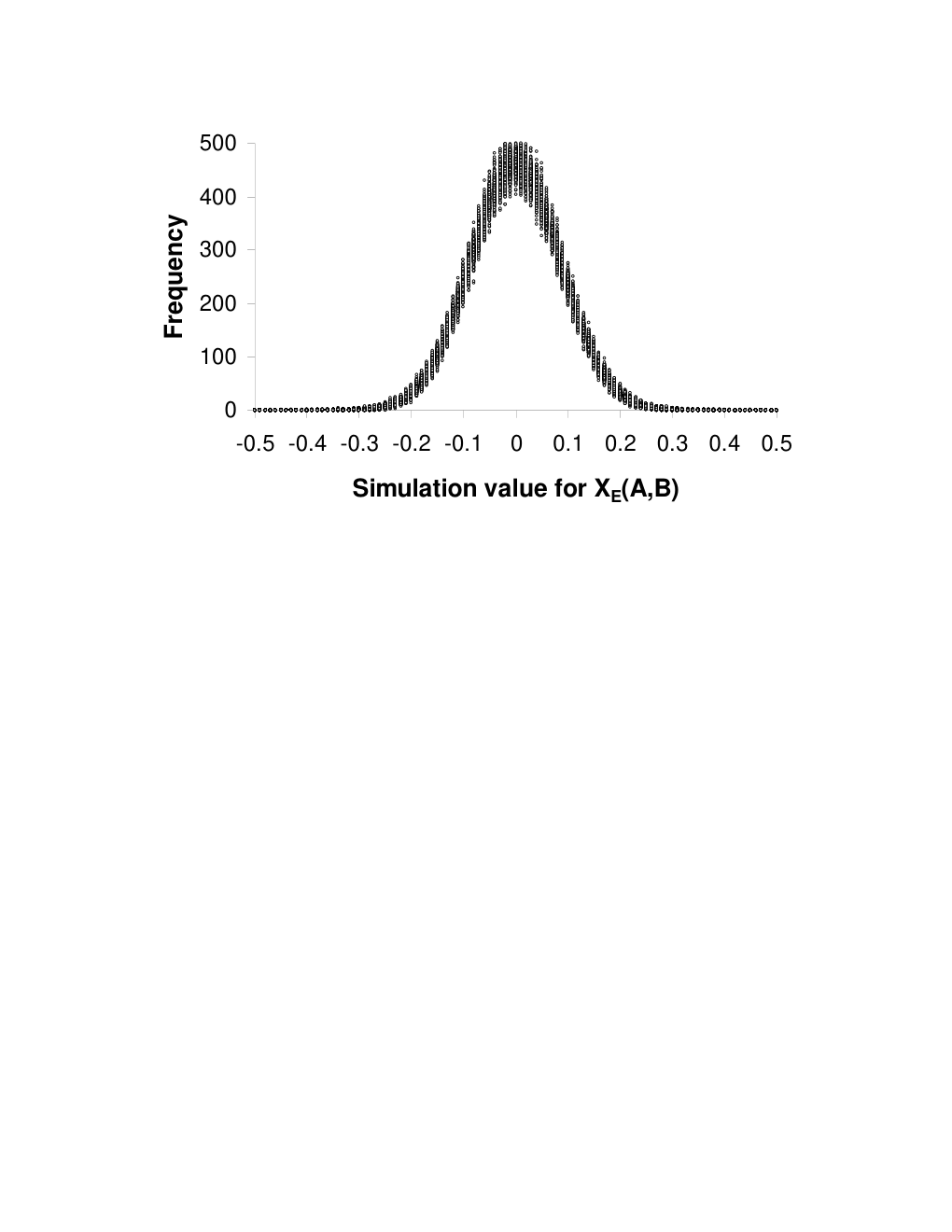
Appendix:
Variance in probability estimates in
the model
In our model, for any event the count of the number of flags in memory that are read as is made up of two components: (i) the number of flags whose value is and which are read correctly as and (ii) the number of flags whose value is but which are read incorrectly as . Since the probability of a flag being read incorrectly is , the first component is a binomial random variable with distribution (where is the number of flags whose true value is and represents the binomal distribution of the number of those flags that are incorrectly read) and the second component is a binomial random variable with distribution (since there are flags whose true value is and represents the binomial distribution of the number of those flags that are incorrectly read as ). We thus have
Since the mean of a binomial distribution is , this gives
as in Equation 3. Since the expected variance of a binomal is , the expected variances of these two distributions are and respectively. Since each read of a flag is an independent Bernoulli trial with probability , these two distributions are independent. For two independent distributions the variance of their difference is equal to the sum of their individual variances and so the expected variance of is
Finally, since variance is defined as the average squared difference from the mean, and since , we get
and the expected variance in the distribution of is a constant for all values of .
It is useful to check this result via simulation. We did this using a program that simulates the effects of random noise in recall on probability estimations for a given set of probabilities (as in Sections 3 and 5). This program took as input an event probability and constructed a ‘memory’ containing items, each item containing a flag indicating whether that item was an example of the given event. The occurrence of those flags in memory matched the given probability . This program also contained a noise parameter ; when reading flag values from memory to generate an estimate , the program was designed to have a random chance of returning the incorrect value. For each input probability ranging from to in steps of the program generated noisy estimates and used these values to estimate .
We carried out this simulation process for a range of values of (, , ). Figure 5 graphs the average variance for these noisy estimates for each value of and for each of those values of . As is clear from the graph, the calculated variance in the simulation was independent of and equal to , as expected.
References
- Ariely, (2009) Ariely, D. (2009). Predictably irrational, revised and expanded edition: the hidden forces that shape our decisions. HarperCollins.
- Bearden and Wallsten, (2004) Bearden, N. J. and Wallsten, T. S. (2004). Minerva-DM and subadditive frequency judgments. Journal of Behavioral Decision Making, 17(5):349–363.
- Bondt and Thaler, (2012) Bondt, W. and Thaler, R. (2012). Does the stock market overreact? The Journal of Finance, 40(3):793–805.
- Bonini et al., (2004) Bonini, N., Tentori, K., and Osherson, D. (2004). A different conjunction fallacy. Mind & Language, 19(2):199–210.
- Bowers and Davis, (2012) Bowers, J. S. and Davis, C. J. (2012). Bayesian just-so stories in psychology and neuroscience. Psychological bulletin, 138(3):389.
- Brunswik, (1955) Brunswik, E. (1955). In defense of probabilistic functionalism: A reply. Psychological Review, 62:236–242.
- Budescu et al., (1988) Budescu, D. V., Weinberg, S., and Wallsten, T. S. (1988). Decisions based on numerically and verbally expressed uncertainties. Journal of Experimental Psychology: Human Perception and Performance, 14(2):281.
- Camerer et al., (2003) Camerer, C., Loewenstein, G., and Rabin, M. (2003). Advances in Behavioral Economics. Princeton University Press.
- Carlson and Yates, (1989) Carlson, B. and Yates, J. (1989). Disjunction errors in qualitative likelihood judgment. Organizational Behavior and Human Decision Processes, 44(3):368–379.
- Cesana-Arlotti et al., (2012) Cesana-Arlotti, N., Téglás, E., Bonatti, L. L., et al. (2012). The probable and the possible at 12 months: intuitive reasoning about the uncertain future. Advances in Child Development and Behavior, 43:1–25.
- Chase, (1998) Chase, R. H. V. M. (1998). Many reasons or just one: How response mode affects reasoning in the conjunction problem. Thinking & Reasoning, 4(4):319–352.
- Chater et al., (2006) Chater, N., Tenenbaum, J. B., and Yuille, A. (2006). Probabilistic models of cognition: Conceptual foundations. Trends in cognitive sciences, 10(7):287–291.
- (13) Costello, F. (2009a). How probability theory explains the conjunction fallacy. Journal of Behavioral Decision Making, 22(3):213–234.
- (14) Costello, F. J. (2009b). Fallacies in probability judgments for conjunctions and disjunctions of everyday events. Journal of Behavioral Decision Making, 22(3):235–251.
- Dawson and Arkes, (1987) Dawson, N. V. and Arkes, H. R. (1987). Systematic errors in medical decision making. Journal of General Internal Medicine, 2:183–187.
- Dougherty et al., (1999) Dougherty, M. R. P., Gettys, C. F., and Ogden, E. E. (1999). Minerva-DM: A memory processes model for judgments of likelihood. Psychological Review, 106(1):180–209.
- Eberhardt and Danks, (2011) Eberhardt, F. and Danks, D. (2011). Confirmation in the cognitive sciences: the problematic case of bayesian models. Minds and Machines, 21(3):389–410.
- Edwards, (1968) Edwards, W. (1968). Conservatism in human information processing. In Kleinmuntz, B., editor, Formal Representation of Human Judgment., pages 17–52. New York: Wiley.
- Endress, (2013) Endress, A. D. (2013). Bayesian learning and the psychology of rule induction. Cognition, 127(2):159 – 176.
- Erev et al., (1994) Erev, I., Wallsten, T. S., and Budescu, D. V. (1994). Simultaneous over- and underconfidence: The role of error in judgment processes. Psychological Review, 101(3):519–527.
- Eva and Norman, (2005) Eva, K. W. and Norman, G. R. (2005). Heuristics and biases: a biased perspective on clinical reasoning. Medical Education, 39(9):870–872.
- Fantino et al., (1997) Fantino, E., Kulik, J., Stolarz-Fantino, S., and Wright, W. (1997). The conjunction fallacy: A test of averaging hypotheses. Psychonomic Bulletin & Review, 4(1):96–101.
- Fiedler, (1988) Fiedler, K. (1988). The dependence of the conjunction fallacy on subtle linguistic factors. Psychological Research, 50(2):123–129.
- Gavanski and Roskos-Ewoldsen, (1991) Gavanski, I. and Roskos-Ewoldsen, D. (1991). Representativeness and conjoint probability. Journal of Personality and Social Psychology, 61(2):181.
- Gigerenzer, (1994) Gigerenzer, G. (1994). Why the distinction between single-event probabilities and frequencies is relevant for psychology and vice versa. In Wright, G. and Ayton, P., editors, Subjective Probability, pages 129–162. Wiley, New York.
- Gigerenzer and Gaissmaier, (2011) Gigerenzer, G. and Gaissmaier, W. (2011). Heuristic decision making. Annual review of psychology, 62:451–482.
- Griffiths and Tenenbaum, (2006) Griffiths, T. L. and Tenenbaum, J. B. (2006). Optimal predictions in everyday cognition. Psychological Science, 17(9):767–773.
- Hasher and Zacks, (1984) Hasher, L. and Zacks, R. (1984). Automatic processing of fundamental information: the case of frequency of occurrence. The American Psychologist, 39(12):1372–1388.
- Hertwig and Gigerenzer, (1999) Hertwig, R. and Gigerenzer, G. (1999). The ‘conjunction fallacy’ revisited: How intelligent inferences look like reasoning errors. Journal of Behavioral Decision Making, 12:275–306.
- Hicks and Kluemper, (2011) Hicks, E. and Kluemper, G. (2011). Heuristic reasoning and cognitive biases: Are they hindrances to judgments and decision making in orthodontics? American Journal of Orthodontics and Dentofacial Orthopedics, 139(3):297–304.
- Hilbert, (2012) Hilbert, M. (2012). Toward a synthesis of cognitive biases: How noisy information processing can bias human decision making. Psychological Bulletin, 138(2):211–237.
- Jones and Love, (2011) Jones, M. and Love, B. C. (2011). Bayesian fundamentalism or enlightenment? on the explanatory status and theoretical contributions of bayesian models of cognition. Behavioral and Brain Sciences, 34(04):169–188.
- Juslin et al., (2009) Juslin, P., Nilsson, H., and Winman, A. (2009). Probability theory, not the very guide of life. Psychological review, 116(4):856–874.
- Kahneman, (2003) Kahneman, D. (2003). Maps of bounded rationality: Psychology for behavioral economics. The American Economic Review, 93(5):1449–1475.
- Kahneman, (2011) Kahneman, D. (2011). Thinking, fast and slow. Macmillan.
- Kheifets and Gallistel, (2012) Kheifets, A. and Gallistel, C. R. (2012). Mice take calculated risks. Proceedings of the National Academy of Sciences, in press.
- Korobkin and Ulen, (2000) Korobkin, R. and Ulen, T. (2000). Law and behavioral science: Removing the rationality assumption from law and economics. California Law Review, 88:1051.
- Marcus and Davis, (2013) Marcus, G. F. and Davis, E. (2013). How robust are probabilistic models of higher-level cognition? Psychological science, 24(12):2351–2360.
- Mellers et al., (2001) Mellers, B., Hertwig, R., and Kahneman, D. (2001). Do frequency representations eliminate conjunction effects? An exercise in adversarial collaboration. Psychological Science, 12(4):269–275.
- Nilsson et al., (2009) Nilsson, H., Winman, A., Juslin, P., and Hansson, G. (2009). Linda is not a bearded lady: Configural weighting and adding as the cause of extension errors. Journal of Experimental Psychology: General, 138(4):517.
- Oaksford and Chater, (2007) Oaksford, M. and Chater, N. (2007). Bayesian rationality: the probabilistic approach to human reasoning. Oxford University Press.
- Richards, (2012) Richards, J. (2012). Psychology of Intelligence Analysis. Pherson Associates.
- Shafir and Leboeuf, (2002) Shafir, E. and Leboeuf, R. A. (2002). Rationality. Annual Review of Psychology, 53(1):491–517.
- (44) Sides, A., Osherson, D., Bonini, N., and Viale, R. (2002a). On the reality of the conjunction fallacy. Memory and Cognition, 30(2):191–198.
- (45) Sides, A., Osherson, D., Bonini, N., and Viale, R. (2002b). On the reality of the conjunction fallacy. Memory & Cognition, 30(2):191–198.
- Sunstein, (2000) Sunstein, C. (2000). Behavioral Law and Economics. Cambridge University Press.
- Tenenbaum et al., (2011) Tenenbaum, J. B., Kemp, C., Griffiths, T. L., and Goodman, N. D. (2011). How to grow a mind: statistics, structure, and abstraction. science, 331(6022):1279–1285.
- (48) Tentori, K., Bonini, N., and Osherson, D. (2004a). The conjunction fallacy: a misunderstanding about conjunction? Cognitive Science, 28(3):467–477.
- (49) Tentori, K., Bonini, N., and Osherson, D. (2004b). The conjunction fallacy: a misunderstanding about conjunction? Cognitive Science, 28(3):467–477.
- Tversky and Kahneman, (1973) Tversky, A. and Kahneman, D. (1973). Availability: A heuristic for judging frequency and probability. Cognitive Psychology, 5:207–232.
- Tversky and Kahneman, (1983) Tversky, A. and Kahneman, D. (1983). Extensional versus intuitive reasoning: The conjunction fallacy in probability judgment. Psychological Review, 90(4):293–315.
- Tversky and Koehler, (1994) Tversky, A. and Koehler, D. (1994). Support theory: A nonextensional representation of subjective probability. Psychological Review, 101(4):547–566.
- Wallsten et al., (1993) Wallsten, T. S., Budescu, D. V., Zwick, R., and Kemp, S. M. (1993). Preferences and reasons for communicating probabilistic information in verbal or numerical terms. Bulletin of the Psychonomic Society.
- Wedell and Moro, (2008) Wedell, D. H. and Moro, R. (2008). Testing boundary conditions for the conjunction fallacy: effects of response mode, conceptual focus, and problem type. Cognition, 107(1):105–136.
- Williams, (2010) Williams, B. (2010). Heuristics and biases in military decision making. Technical report, DTIC Document.