1–5
Solar-like differential rotation and equatorward migration in a convective dynamo with a coronal envelope
Abstract
We present results of convective turbulent dynamo simulations including a coronal layer in a spherical wedge. We find an equatorward migration of the radial and azimuthal fields similar to the behavior of sunspots during the solar cycle. The migration of the field coexist with a spoke-like differential rotation and anti-solar (clockwise) meridional circulation. Even though the migration extends over the whole convection zone, the mechanism causing this is not yet fully understood.
keywords
MHD, Sun: magnetic fields, Sun: activity, Sun: rotation, turbulence1 Introduction
The Sun shows an activity cycle with a period of eleven years, which is manifested by sunspots occurring on the solar disk. Every eleven years the number of sunspots has a maximum and around five years later a minimum. With each cycle the polarity of the global magnetic field changes sign and gives rise to the 22 years Hale cycle. The occurrence of sunspots does not only vary with time, but it also shows a strong latitudinal dependence. During solar minimum, the sunspots are more likely to emerge at higher latitudes and during the maximum at lower latitudes, close to the equator. This observed feature corresponds to an equatorward migration of the magnetic activity belt causing the sunspots. Producing the cyclic behavior in numerical simulations is challenging. Either one neglects important backreaction of the magnetic field on the fluid motions and solves the problem in a kinematic mean-field approach with widely varying parameterizations for the small scales (Dikpati & Charbonneau, 1999; Käpylä et al., 2006; Kitchatinov & Olemskoy, 2012, e.g.) or one uses direct numerical simulations (DNS) with orders of magnitudes too high viscosity and diffusivity, and too low stratification of density and temperature (Brun et al., 2004; Ghizaru et al., 2010; Käpylä et al., 2010, e.g.). The kinematic mean-field approach seems to be successful in reproducing observed features of the Sun. However, whether solar activity is generated by a distributed turbulent dynamo throughout the convection zone or in a thin layer below the convection zone is still very much under debate and cannot be answered just by mean-field modeling. It has turned out to be much more challenging to obtain solar-like magnetic activity from DNS or large-eddy simulations: models either show only weak mean fields (Brun et al., 2004), strong quasi-steady large-scale fields (Brown et al., 2010), cycles but no migration (Ghizaru et al., 2010), or cycles and poleward migration (Gilman, 1983; Käpylä et al., 2010; Brown et al., 2011). Recently Käpylä et al. (2012) were able to reproduce an equatorward migration of the azimuthal and radial magnetic fields for the first time using direct numerical simulation of a convective dynamo.
Another important observed feature of the Sun is its differential rotation. It is broadly believed that the solar differential rotation is an important ingredient in the solar dynamo. In the kinematic models the differential rotation profile is used as an input parameter. Beside mean-field models (Kitchatinov & Rüdiger, 1999, e.g.), a solar-like differential rotation profile has not yet been self-consistently obtained in direct numerical simulations. Often the rotation profile is solar-like in the sense that the equator rotates faster than the poles (Brun et al., 2004; Käpylä et al., 2011, e.g.), but the angular velocity is constant on cylinders due to the Taylor-Proudman balance. Spoke-like rotation has not been seen unless a latitudinal temperature gradient is imposed at the base of the convection zone (Miesch et al., 2006).
In the following work, we present the results of a two-layer model, which combines a convection zone with a coronal layer. The model was originally developed to investigate coronal ejections generated by a dynamo underneath the surface and the helicity flux due to the coronal envelope and the ejections, see Warnecke & Brandenburg (2010) and Warnecke et al. (2011); Warnecke et al. (2012a); Warnecke et al. (2012b) for details. In this work we focus on the magnetic and fluid properties in the convection zone. The dynamics of coronal ejections will be discussed in a followup paper.
2 The model

We use a similar setup as in Warnecke et al. (2012b), which we improve in two respects. Firstly, we apply more solar-like temperature and density profiles for the coronal layer. In the earlier work, the temperature in the corona was constant and identical with that in the photosphere. Now, we let the temperature rise above the surface reaching a constant value at a radius of , where is the solar radius. The coronal temperature is 1.2 times larger than that at the base of the convection zone. In Figure 1 the radial profiles of density, temperature, pressure, and entropy are shown from the saturated stage of the simulation. The entropy is negative in the convection zone with a negative slope. Close to the surface () the gradient changes sign resulting in positive values above . The density decreases exponentially in the corona (). In the convection zone () the stratification is initially isentropic. This results in a density difference in the convection zone and in the entire domain, where , and . The other improvement is to use a turbulent heat conductivity in the entropy equation (4) to model the unresolved heat conductivity. Similar subgrid-scale models have also been used by e.g. Brun et al. (2004) and Käpylä et al. (2011) to significantly increase energy transport due to the convective flux. We apply a constant value of , which is similar to the molecular viscosity , in the interval of , and tends smoothly to zero above and below.
We use a spherical wedge extending from to in radial direction, from to in colatitude, and from to in azimuthal direction. We solve the following equations of compressible magnetohydrodynamics:
| (1) | |||||
| (2) | |||||
| (3) | |||||
| (4) |
where magnetic field is expressed by , where is the vector potential, and is the magnetic diffusivity. Furthermore, is the velocity, is the density and is the gravitational acceleration. The Coriolis and Lorentz forces are given by and , respectively, where is the angular velocity and is the current density. is the traceless rate-of-strain tensor and is the kinematic viscosity. The energy conservation equation is solved in terms of the specific entropy . We include radiative transport in term of the diffusion approximation with heat conductivity and model the unresolved turbulent transport with . The fluid obeys the ideal gas law, , where is the ratio of specific heats at constant pressure and constant volume, respectively, and is the internal energy density, which defines the temperature . The third and fourth terms on the rhs of Equation (4) describe viscous and Ohmic heating. The radial cooling function is defined such that it cools/heats the corona towards a predefined temperature profile , which is plotted in Figure 1. As an initial condition we use a stratification profile similar to that plotted in Figure 1 and a weak, random, Gaussian-distributed seed magnetic field in the convection zone.
We apply periodic boundary conditions in the azimuthal direction. For the velocity field we use stress-free conditions on all other boundaries. For the magnetic field we use a perfect conductor boundary condition at the and both boundaries; at the boundary be apply a vertical-field condition. The heat flux through the lower () boundary is held constant and the temperature at the top is fixed.
We employ the Pencil Code11 1 http://pencil-code.googlecode.com, which uses sixth-order centered finite differences in space and a third-order Runge-Kutta scheme in time; see Mitra et al. (2009) for the extension to spherical coordinates.
3 Results
For this work we consider a single simulation, which is defined by the following properties: the Coriolis number is 14, the Reynolds number is , and the magnetic Prandtl number . Here is the wavenumber of the energy carrying scales and is defined as , and is the rms velocity at radius .


Below the surface () the domain is convectively unstable. The resulting convective motions drive a turbulent dynamo and generate a large–scale magnetic field. The rms magnetic field in the convection zone reaches 0.38 times the equipartition field . In Figure 2 we plot the azimuthally averaged (in the following mean) radial and azimuthal magnetic fields as functions of time in terms of the turnover time . Effectively is an eddy turnover time, which varies between a few minutes and more than a month in the solar convection zone, depending on the depth. In the kinematic regime, the magnetic field pattern shows a cyclic poleward migration close to the surface () for the azimuthal and radial fields at lower latitudes. The period is short, only a few tens . In the non-linear regime, a new pattern is developing: equatorward migration starting at high latitudes overcomes the poleward migration at low latitudes. This equatorward migration shows a longer period of 100-200 . Additionally the pattern is not only visible near the surface, as it penetrates into the convection zone as shown in the left panel of Figure 2. The pattern does not look as regular as in Käpylä et al. (2012), which can be explained by the interaction of the corona and convection zone.
Initially the interior rotation profile is constant in cylinders with a positive gradient of angular velocity at low latitudes. In the hydrodynamic state, affected by rotation, the convective turbulence re-shapes the rotation profile within the convection zone, while in the convectively stable coronal layer only viscosity is at play. After a dynamically important magnetic field has been generated by the dynamo action, it influences the rotation as well. In the corona, where the density is much lower than in the convection zone, the Lorentz force can dominate over the Coriolis force, see Equation (4), and have a greater influence on the angular velocity. In our simulation the velocities in the corona saturate not before .
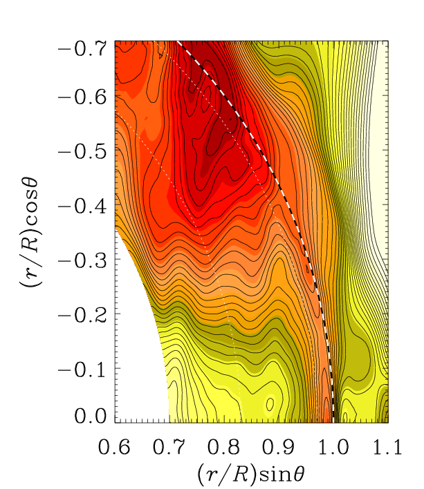
The differential rotation profile is solar-like, see Figure 3. The equator rotates faster than the poles and the contours of constant rotation show a spoke-like pattern–especially at low latitudes. This is the first time a spoke-like profile has been found in DNS in combination with equatorward migration. Käpylä et al. (2012), whose setup is similar to ours in the convection zone, found that the contours of constant rotation are significantly more cylindrical at similarly high Coriolis numbers. This could be due to the interaction between the coronal layer and the convection zone. There might be even an indication of a surface shear layer at latitudes . The meridional circulation shows a clockwise pattern–in contrast to the Sun. Instead of a poleward flow near the surface, as in the Sun, the flow is equatorward. This might be one possible explanation for the equatorward migration of the magnetic field. The field would then be dragged along with the fluid motion to the equator. But the magnetic field shows an equatorward migration throughout the convection zone, and the anti-solar meridional circulation seems to be shallow with a return flow in the middle of the convection zone. In our simulation the meridional circulation seems not to have a connection with the equatorward migration and the generation of the field.

Another possible explanation of the equatorward migration can be the profile of the effective which likely generates the mean magnetic field . has two contributions
| (5) |
proportional to the kinetic helicity density and the magnetic helicity density , respectively, and where is a correlation time of the turbulence and can be expressed by the eddy turnover time . In Figure 4, we show the two contribution as functions of radius for two latitudes. In the convection zone is dominated by the kinetic contribution and is influenced by only close to the surface. One reason behind the equatorward migration could be the different values of at different latitudes. We observe a tendency for the effect to have larger values at higher latitudes. The latitudinal profile of could cause the mean field to migrate towards the equator. This has to be verified by comparison with simulations which show a poleward migration.


4 Conclusions
In summary, we use a two-layer model that combines self-consistent convective dynamo action with a coronal layer, resulting in equatorward migration of the mean magnetic field. A solar-like rotation profile with spoke-like contours at low latitudes is generated. This is different from recent results of Käpylä et al. (2012) with a similar model, but without corona. In forthcoming work, we will study the mean magnetic field structure and differential rotation for different rotation rates and investigate the cause of equatorward migration in more detail.
References
- Brown et al. (2010) Brown, B. P., Browning, M. K., Brun, A. S., Miesch, M. S., & Toomre, J. 2010, ApJ, 711, 424
- Brown et al. (2011) Brown, B. P., Miesch, M. S., Browning, M. K., Brun, A. S. & Toomre, J. 2011, ApJ, 731, 69
- Brun et al. (2004) Brun, A. S., Miesch, M. S., & Toomre, J. 2004, ApJ, 614, 1073
- Dikpati & Charbonneau (1999) Dikpati, M., & Charbonneau, P. 1999, ApJ, 518, 508
- Ghizaru et al. (2010) Ghizaru, M., Charbonneau, P., & Smolarkiewicz, P. K. 2010, ApJL, 715, L133
- Gilman (1983) Gilman, P. A. 1983, ApJS, 53, 243
- Käpylä et al. (2006) Käpylä, P. J., Korpi, M. J. & Tuominen, I. 2006, AN, 327, 884
- Käpylä et al. (2010) Käpylä, P. J., Korpi, M. J., Brandenburg, A., Mitra, D. & Tavakol, R. 2010, AN, 331, 73
- Käpylä et al. (2011) Käpylä, P. J., Korpi, M. J., Guerrero, G., Brandenburg, A. & Chatterjee, P. 2011, A&A, 531, A162
- Käpylä et al. (2011) Käpylä, P. J., Mantere, M. J., & Brandenburg, A. 2011, Astron. Nachr., 332, 883
- Käpylä et al. (2012) Käpylä, P. J., Mantere, M. J., & Brandenburg, A. 2012, ApJL, 755, L22
- Kitchatinov & Rüdiger (1999) Kitchatinov, L. L. & Rüdiger, G. 1999, A&A, 344, 911
- Kitchatinov & Olemskoy (2012) Kitchatinov, L. L. & Olemskoy, S. V. 2012, Solar Phys., 276, 3
- Miesch et al. (2006) Miesch, M. S., Brun, A. S. & Toomre, J. 2006, ApJ, 641, 618
- Mitra et al. (2009) Mitra, D., Tavakol, R., Brandenburg, A., & Moss, D. 2009, ApJ, 697, 923
- Warnecke & Brandenburg (2010) Warnecke, J., & Brandenburg, A. 2010, A&A, 523, A19
- Warnecke et al. (2011) Warnecke, J., Brandenburg, A., & Mitra, D. 2011, A&A, 534, A11
- Warnecke et al. (2012a) Warnecke, J., Brandenburg, A., & Mitra, D. 2012a, JSWSC, 2, A11
- Warnecke et al. (2012b) Warnecke, J., Käpylä, P. J., Mantere, M. J., & Brandenburg, A. 2012b, Solar Phys., 280, 299