Experimental Test of Universal Complementarity Relations
Abstract
Complementarity restricts the accuracy with which incompatible quantum observables can be jointly measured. Despite popular conception, the Heisenberg uncertainty relation does not quantify this principle. We report the experimental verification of universally valid complementarity relations, including an improved relation derived here. We exploit Einstein-Poldolsky-Rosen correlations between two photonic qubits, to jointly measure incompatible observables of one. The product of our measurement inaccuracies is low enough to violate the widely used, but not universally valid, Arthurs-Kelly relation.
pacs
42.50.Xa; 03.65.Ta; 03.65.UdIntroduction.—Niels Bohr repeatedly emphasised that the fundamental distinction between quantum and classical mechanics is the principle of complementarity, which states that the experimental arrangements required to accurately measure two different observables are, in general, incompatible [1]. Indeed, in replying to the famous critique by Einstein, Podolsky and Rosen on the completeness of the quantum theory [2], Bohr stated that “it is only the mutual exclusion of any two experimental procedures, permitting the unambiguous definition of complementary physical quantities, which provides room for new physical laws” [3].
It is commonly thought that Bohr’s complementarity principle is captured by Heisenberg-type uncertainty relations such as , where () is the predicted spread of a perfect position (momentum) measurement, arising from the underlying position (momentum) spread of a particle’s wave function. However, this relation does not reflect the impossibility of performing such perfect measurements at the same time. Nor do measurement-disturbance relations [4, 5, 6, 7], since these refer to sequential rather than joint measurements. By contrast, a complementarity relation should restrict the degree of accuracy with which position and momentum — or indeed any two incompatible quantities — can be measured simultaneously.
In particular, whereas two incompatible observables and are not jointly measurable with perfect accuracy, one may still make inaccurate joint estimates, and , where and are compatible. In quantum mechanics, physical quantities can always be represented by Hermitian operators (in some Hilbert space), and the above statements imply but . The key question then concerns the quality of these jointly-measurable estimators: how close are they to the original observables of interest? A natural measure of inaccuracy is the root mean square error, [8, 9]. This measure vanishes for a perfect estimate, , and more generally quantifies the degree to which the estimator deviates from the quantity being estimated [10].
Arthurs and Kelly showed in 1965 that for any joint estimates of position and momentum that are globally unbiased, i.e., for which the average values of the estimators are equal to the average values of the corresponding observables for every state [11]. This relation was subsequently generalized to the complementarity relation [9, 12, 13]
| (1) |
valid for globally-unbiased joint estimates of any two observables and . Here , and is nonzero only if and are incompatible. Thus, the more accurately a globally-unbiased joint measurement can estimate observable , the less accurately it can estimate an incompatible observable , and vice versa. Other complementarity relations—also called joint-measurement uncertainty relations—have been given, using alternative measures of inaccuracy, but are again only valid for restricted classes of measurements [14, 15, 16, 17, 18, 19, 20].
The above-mentioned complementarity relations not only lack universal validity but, most importantly, are inapplicable in cases of considerable physical interest. For example, Einstein, Podolsky and Rosen (EPR) based their argument for the incompleteness of quantum theory on the case of two particles having highly correlated positions and momenta [2]. In this case, one can make highly accurate joint estimates of the position and momentum of the first particle via, for example, a position measurement on the first particle and a momentum measurement on the second. Thus, the Arthurs-Kelly relation (1) clearly fails in the EPR scenario.

Indeed, it is only relatively recently that universally valid complementarity relations have been given, holding for arbitrary joint estimates of two observables in any measurement scenario. In particular, following related work by Ozawa on measurement-disturbance relations [4], Hall showed that the inaccuracies of any estimates generated by a joint measurement of observables and must satisfy [21]
| (2) |
where is the spread in quantity . Thus, unlike Eq. (1), the inaccuracies can both be arbitrarily small, provided the spreads of the estimates are sufficiently large. This is a consequence of not imposing global unbiasedness: for a given state one can now tailor joint estimation schemes to the specific state of interest (where these schemes may perform quite poorly for other states), so as to reduce the inaccuracies. However, the spreads will be correspondingly increased. The above EPR scenario provides such a tailored estimation scheme, for position and momentum, which saturates Eq. (2) [21]. Hall also determined the form of the optimal estimates of and in any given measurement scenario, i.e., those functions of the measurement data that yield estimators and with the smallest possible inaccuracies and [21, 22].
Ozawa has given a formally similar relation [23]
| (3) |
This differs from Eq. (2) in depending on the spreads and of the observables, rather than on the actual measured spreads and , but similarly implies that the inaccuracies cannot both be zero for incompatible observables. The Hall relation implies (and hence is stronger than) the Ozawa relation for the particular case of optimal estimators, for which [21, 22].
Here we provide the first experimental test of universal complementarity relations, in an EPR-type scenario for which the Arthurs-Kelly relation (1) is shown to be violated. Moreover, a new universal complementarity relation, which is stronger than both the Hall and Ozawa relations for optimal estimates, is proved here and similarly tested. The measurement inaccuracies are determined by generalizing the Lund-Wiseman method [24] (recently implemented in the context of measurement–disturbance relations [7]), by using the contextual value formalism [25] to allow the replacement of a weak measurement interaction by one of arbitrary strength.
Stronger universal complementarity relation.—In addition to experimentally investigating the complementarity relations (1)–(3), we also tested the relation
| (4) |
which we have derived (see the Supplemental Material [26]). Unlike Eqs. (1)–(3), this relation does not involve an term, and so directly quantifies the tradeoff between inaccuracy and spread. It similarly implies that and cannot both vanish for incompatible and .
The complementarity relation (4) is clearly stronger than a simple average of Eqs. (2) and (3), and strictly implies each of the latter in the case where optimal estimates are made from the measurement data [26]. It is also stronger, in the sense of lying closer to the bound, for all estimators considered in our experiment.
Experimental setup.—To provide a discrete analogy of the EPR scenario discussed in the introduction, we generated pairs of optical polarisation qubits (see Fig. 1) having high fidelity with the entangled state
| (5) |
Here and refer to horizontal and vertical polarisation, which are assigned as eigenstates of the polarisation operator [27]. Observables and in the complementarity relations (1)-(4) are chosen to be the [diagonal (anti-diagonal)] and [right-(left-)circular] polarisations of the first qubit.
The state is maximally entangled for , allowing perfectly accurate joint estimates of and (via measuring directly, and the polarisation of the perfectly anticorrelated second qubit), analogous to the EPR example. However, the lower bound of the complementarity relations, , trivially vanishes. Conversely, the choice (or ) maximises , but corresponds to a factorisable state from which no information about the the first qubit can be gained via a measurement on the second. Hence, the intermediate choice was made for our experiment. Quantum state tomography [28] on the state generated by a spontaneous parametric down-conversion source gave a fidelity of with the desired entangled state (see the Supplemental Material [26]).
We demonstrate how to experimentally use semiweak measurements, in conjunction with strong measurements, to operationally determine the inaccuracy . The aim of the experiment is to jointly estimate the and polarisations of the first qubit. One could directly measure on the first qubit, and estimate by applying some function to the outcome of a polarisation observable measured on the second qubit [see Fig. 1(a)]. However, to allow the corresponding inaccuracies to be determined, the first qubit was also subjected to an initial semiweak measurement process [29] [see Fig. 1(b)], implemented using the polarisation dependence of Fresnel reflection from a glass slide [30] oriented at an angle [see Fig. 1(c)]. While weak measurements are measurements that introduce negligible disturbance to a system while providing an infinitesimal amount of information, semiweak measurements provide small but finite information about the system, with small but non-negligible back action.
The slide reflects (transmits) horizontal and vertical polarisations with probabilities and ( and ), found by direct measurement to be and . Wave plates before and after the slide were adjusted to rotate the basis of the semiweak measurement from to . The strength of the measurement is quantified by . The above values of and give , indicating that is semiweak.
Measuring the inaccuracies.—The outcome of the semiweak measurement, or , occurs with some probability , and probes the polarisation of the first qubit. It has a unique associated numerical value, , called the contextual value of [25], defined by the property , thus generalising the notion of eigenvalues to semiweak measurements. The contextual values are simple functions of and (see the Supplemental Material [26] and Ref. [30]). As shown in the Supplemental material [26], they allow the inaccuracy of any estimator of the form to be experimentally determined via the formula
| (6) |
Here is the measured joint probability of outcomes , and for the binary measurements , and , respectively, and . Equation (6) reduces to Eq. (16) of Ref. [24] in the weak limit, .
It would be possible to similarly determine the inaccuracy of the estimator by rotating the basis of the semiweak measurement from to . However, this inaccuracy can instead be inferred by taking into account the effect of on the first qubit [Fig. 1(b)]. In particular, as shown in the Supplemental Material [26], the measurement of subsequent to is equivalent to a generalized measurement on the initial state, described by a positive-operator-valued measure , with . The inaccuracy of the estimator corresponding to follows as , irrespective of the input state (see the Supplemental Material [26]). Note the inaccuracy vanishes in the weak limit .
Experimental results.—The joint probability distribution was measured for several choices of the polarisation observable , corresponding to the Bloch sphere angles and , and . For state in (5), and correspond to the observable of the second qubit that is most strongly correlated with the polarisation of the first, in the sense of maximising . Data were collected for 30 s per setting, with a total measured flux of 2000 coincidence counts per second (see the Supplemental Material [26]).
Two types of estimates for , based on the outcome of the measurement, were considered. The first type corresponded to simply estimating to be , i.e., , which is the best possible if is constrained to have the same eigenvalues as . The second type of estimate exploited the tomographically determined state of the source, , to make the optimal estimate, , corresponding to the smallest possible inaccuracy, with [21]
For example, for defined by and , and .
The inaccuracies were determined via Eq. (6), and are plotted in Fig. 2. It is also verified in Fig. 2 that the inaccuracy and spread of satisfy Hall’s inaccuracy–dispersion relation
| (7) |
for optimal estimates [21].
The spreads and were calculated directly from the measured distribution , while we obtained , , and from . Combined with the above inaccuracy data, this allowed complementarity relations (1)–(4) to be tested for the two types of estimate of . The universal complementarity relations (2)–(4) were validated and the Arthurs-Kelly relation (1) strongly violated (Fig. 3). The latter violation was expected for EPR scenarios, as discussed in the introduction. Fig. 3(b) also verifies that, for optimal estimates, the new complementarity relation (4) is stronger than relations (2) and (3), as expected.
Discussion—Universal complementarity relations should hold for any joint measurement of two observables. We have provided the first experimental investigation of such relations (Fig. 3). This was done in an EPR-type scenario, for which the Arthurs-Kelly relation (1) is violated. We have, furthermore, derived and verified a new universal complementarity relation, Eq. (4), that is significantly stronger than the previously obtained relations (2) and (3) for the case of optimal estimators. We have also verified the inaccuracy–dispersion relation (7) for optimal estimators.
It would be of interest to also test the universal complementarity relations for the case of continuously valued quadrature observables and . This would allow the relations to be explored in a context more akin to the original scenario envisaged by EPR [2], with the advantage of a saturable and fixed lower bound [21].
Our work represents an important advance in the quantitative understanding and experimental verification of complementarity, arguably the most important foundational principle of quantum mechanics. This principle underlies many aspects of quantum information technology, ranging from entanglement verification [31] to quantum dense coding [32] to the security of quantum cryptography [33], and our work could have implications in all these areas.
Acknowledgements.
Acknowledgments—MMW thanks Dylan Saunders, Adam Bennet, Allen Boston and Sacha Kocsis for helpful contributions. MJWH thanks Cyril Branciard for pointing out the difference between the joint uncertainty relations in Refs. [21] and [23], and for stimulating discussions. We are grateful to Yutaka Shikano and Masanao Ozawa for drawing our attention to relevant literature. This research was supported by the ARC Centre of Excellence CE110001027.References
- [1] N. Bohr, Atomic Physics and Human Knowledge (Wiley, New York, 1958), pp. 32-66.
- [2] A. Einstein, B. Podolsky, and N. Rosen, Phys. Rev. 47, 777 (1935).
- [3] N. Bohr, Phys. Rev. 48, 696 (1935).
- [4] M. Ozawa, Phys. Rev. A 67, 042105 (2003).
- [5] M. Ozawa, Ann. Phys. (Amsterdam) 311, 350 (2004).
- [6] J. Erhart, S. Sponar, G. Sulyok, G. Badurek, M. Ozawa, and Y. Hasegawa, Nature Phys. 8 185 (2012).
- [7] L. A. Rozema, A. Darabi, D. H. Mahler, A. Hayat, Y. Soudagar, and A. M. Steinberg, Phys. Rev. Lett. 109, 100404 (2012).
- [8] H. L. van Trees, Detection, Estimation and Modulation Theory Part 1 (Wiley, New York, 2001), Sec. 2.4.
- [9] M. Ozawa, in Quantum Aspects of Optical Communications, (eds C. Bendjaballah, O. Hirota, and S. Reynaud) Lecture Notes in Physics 378 (Springer, Berlin, 1991), pp. 3-17.
- [10] Note the estimates referred to here are of observables, and hence are represented by operators. They should not be confused with estimates of classical parameters of quantum states, the theory of which was pioneered by Helstrom and Holevo [34].
- [11] E. Arthurs and J. L. Kelly, Jr., Bell Syst. Tech. J. 44, 725 (1965).
- [12] E. Arthurs and M. S. Goodman, Phys. Rev. Lett. 60, 2447 (1988).
- [13] S. Ishikawa, Rep. Math. Phys. 29, 257 (1991).
- [14] W. K. Wootters and W. H. Zurek, W. H., Phys. Rev. D 19, 473 (1979).
- [15] H. Martens and W. de Muynck, Found. Phys. 20, 357 (1990).
- [16] G. Jaeger, A. Shimony, and L. Vaidman, Phys. Rev. A 51, 54 (1995).
- [17] D. M. Appleby, Int. J. Theor. Phys. 37, 1491 (1998).
- [18] A. Trifonov, G. Björk, and J. Söderholm, Phys. Rev. Lett. 86, 4423 (2001).
- [19] P. Busch and C. R. Shilladay, Phys. Rev. A 68, 034102 (2003).
- [20] Y. Watanabe, T. Sagawa and M. Ueda, Phys. Rev. A 84, 042121 (2011).
- [21] M. J. W. Hall, Phys. Rev. A 69, 052113 (2004).
- [22] M. J. W. Hall, Phys. Rev. A 64, 052103 (2001).
- [23] M. Ozawa, Int. J. Quantum Inf. 01, 569 (2003); M. Ozawa, Phys. Lett. A 320, 367 (2004).
- [24] A. P. Lund and H. M. Wiseman, New. J Phys. 12, 093011 (2010).
- [25] J. Dressel, S. Agarwal, and A. N. Jordan, Phys. Rev. Lett. 104, 240401 (2010).
- [26] See appended Supplemental Material for derivation of theoretical results and further experimental details.
- [27] H. M. Wiseman and G. J. Milburn, Quantum Measurement and Control (Cambridge University Press, Cambridge, 2010).
- [28] A. G. White, A. Gilchrist, G. J. Pryde, J. L. O’Brien, M. J. Bremner, and N. K. Langford, JOSA B 24, 172 (2007).
- [29] G. J. Pryde, J. L. O’Brien, A. G. White, T. C. Ralph, and H. M. Wiseman, Phys. Rev. Lett. 94, 220405 (2005).
- [30] J. Dressel, C. J. Broadbent, J. C. Howell, and A. N. Jordan, Phys. Rev. Lett. 106, 040402 (2011).
- [31] F. Buscemi, Phys. Rev. Lett. 108, 200401 (2012).
- [32] C. H. Bennett and S. J. Wiesner, Phys. Rev. Lett. 69, 2881 (1992).
- [33] N. Gisin, G. Ribordy, W. Tittel, and H. Zbinden, Rev. Mod. Phys. 74, 145 (2002).
- [34] C. W. Helstrom, Quantum Detection and Estimation Theory (Academic Press, New York, 1976); A. S. Holevo, Probabilistic and Statistical Aspects of Quantum Theory (North-Holland, Amsterdam, 1982).
- [35] C. Branciard, Proc. Nat. Acad. Sci., 110 6742 (2013).
- [36] R. Rangarajan, M. Goggin, and P. Kwiat, Opt. Express 17, 18920 (2009).
- [37] P. G. Kwiat, E. Waks, A. G. White, I. Appelbaum, and P. H. Eberhard, Phys. Rev. A 60, R773 (1999).
- [38] H. Margenau and R. N. Hill, Prog. Theor. Phys. 26, 722 (1961).
- [39] M. Ozawa, Phys. Lett. A 335, 11 (2005).
- [40] H. M. Wiseman, Phys. Lett. A 311, 285 (2003).
- [41] K. Kraus, States, Effects and Operations (Springer, Berlin, 1983).
Supplemental Material
I Proof of Eq. (4)
Any two joint estimates of observables and may be represented by two commuting operators and on a suitable Hilbert space (via a Naimark extension if necessary) [21, 23]. It follows that , and hence, using the triangle inequality, that
Applying the Schwarz inequality (which lies behind all such relations), , with and suitably chosen from , and , leads to Eq. (4) as desired.
Eq. (4) is stronger than complementarity relations (2) and (3), both in the sense of implication and of having a smaller left hand side, for the case that optimal estimates and are made [corresponding to those functions of the measurement data that yield the smallest possible inaccuracies and . This follows from the inaccuracy-dispersion relations and for optimal estimates [21]. In particular, and , and hence Eq. (4) implies Eq. (3) for such estimates. Further, defining and , then , and the difference of the left hand sides of relations (2) and (4) is , where is never less than zero. Hence Eq. (4) also implies Eq. (2) for optimal estimates, as claimed.
It is of interest to note that if denotes the disturbance to an observable , caused by making an estimate of that changes to [4, 5], then one may similarly derive a measurement-disturbance uncertainty relation,
as will be discussed elsewhere. We note also that new joint-measurement and measurement-disturbance relations have recently been given by Branciard [35].
II Photon source
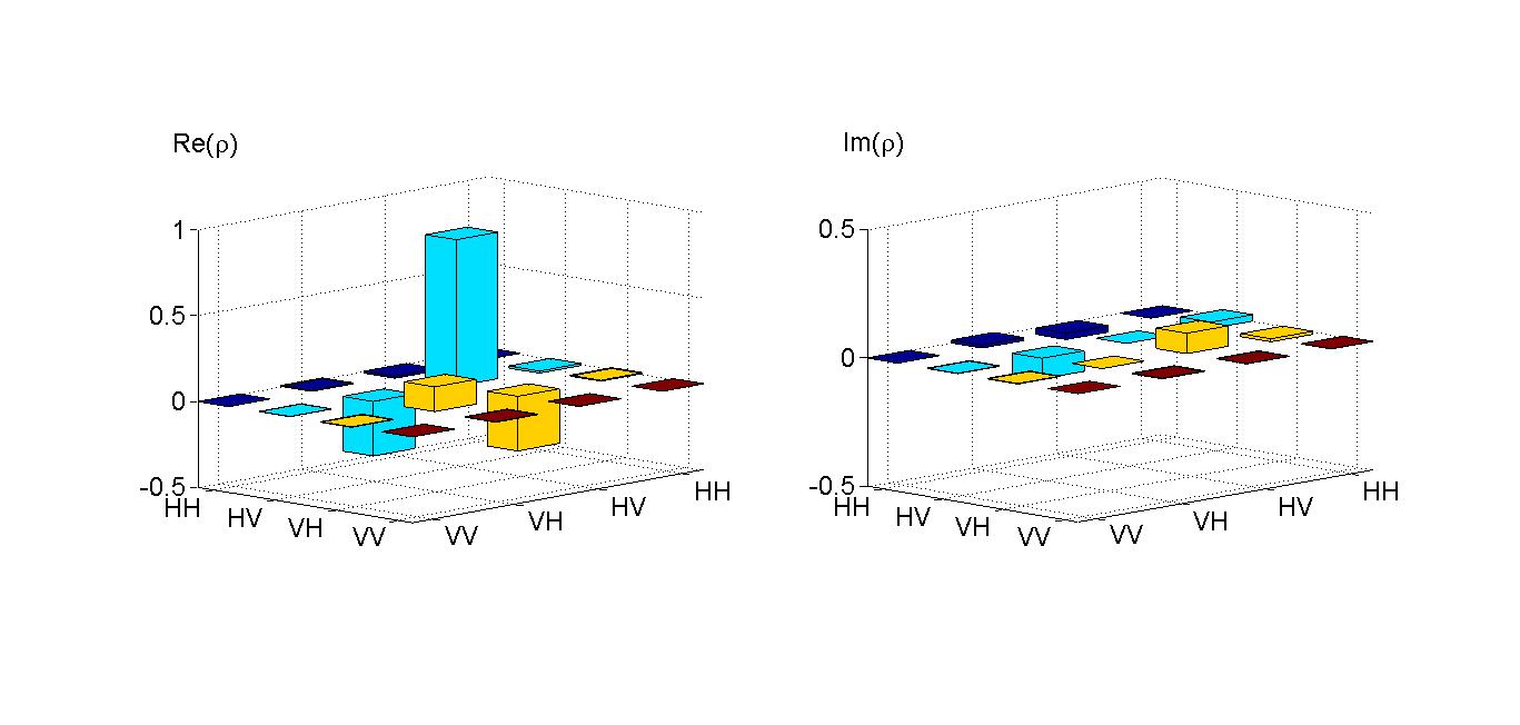
A 120 mW, linearly polarised continuous wave 404 nm laser diode was used to pump a pair of 0.5 mm thick Bismuth Borate (BiBO) crystals. The crystal pair is oriented such that the optical axes of the pair are crossed in what is known as a ‘sandwich’, and an additional BiBO crystal is inserted into the pump to precompensate the temporal walkoff between H and V polarisations in the downconversion crystal [36, 37]. When pumped with diagonally polarised light, spontaneous parametric down conversion leads to photon pairs at 808 nm in the maximally entangled state. By adjusting a half wave plate inserted into the pump beam before the crystal (Fig. 1(c) of the main paper), we can tune (Eq.(5)). To convert to , we must also change the -basis correlation and the phase of the superposition, which we do by applying an and a operation to one of the qubits. Experimentally, we implement these operations on the first qubit using wave plates immediately following the SPDC source, as shown in Fig. 1(c) of the main paper. Counting in coincidence with a 3 ns window and 3 nm FWHM interference filters, photon pair rates of s-1 were observed. Quantum tomography was used to reconstruct the state produced by the source, as shown in Fig. 4.
III Data and and error analysis
The measured relative frequencies for the outcomes of , and in Fig 1(b) of the main text are shown in Table I below. Uncertainties predominantly arise from Poissonian counting statistics due to the random SPDC generation times, and slow, small thermal drifts in the fibre coupling leading to changes in and during the data collection. The latter effect was characterized by measuring these quantites before and after the data collection, and observing the mean and spread of the values. Uncertainties in directly measured experimental values were combined using standard error propagation formulae to generate uncertainties in values calculated from the data. The small deviations between experiment and theory are attributed to a combination of inexact wave plate settings and other uncompensated small thermal drifts (e.g. fibre birefringence) in the experiment.
IV Contextual values for the semiweak measurement
As noted in the main text, contextual values for the outcomes of semiweak measurements were introduced by Dressel et al., and generalise the notion of eigenvalues for projective measurements [25, 30]. As was further noted, the contextual values and of the semiweak measurement in Fig. 1(b), corresponding to reflection and transmission by the glass slide in Fig. 1(c), are defined by the property , where and denote the probability of reflection and transmission, respectively.
To determine , note that the operation of the glass slide, combined with wave plates before and after it to rotate the measurement basis from the polarisation to the polarisation, corresponds to a (semiweak) polarisation-dependent beamsplitter. As per Dressel et al. [30] (who analysed the case of polarisation), the action of on any input qubit state is therefore described by the completely-positive trace-preserving map
| (8) |
where the corresponding measurement operators and are Hermitian with , with denoting and the unit operator. The probabilities of reflection and transmission follow as . The equation may then be solved for the contextual values and , to give [30]
| (9) |
Note that in the ‘strong’ limit , corresponding to perfect discrimination of the eigenstates of by the measurement , the contextual values are equal to the associated eigenvalues of . Conversely, in the ‘weak’ limit , corresponding to polarisation-independent operation, with no information about able to be gained from the measurement , the contextual values become unbounded. For the measured values of and in our experiment (given in the main text), the associated contextual values follow as and .
V Determining inaccuracies from semiweak measurements
To test the validity or otherwise of complementarity relations (1)–(4), it is necessary to experimentally determine the inaccuracies and . This problem has been previously discussed in context of measurement–disturbance uncertainty relations, which also involve the inaccuracy of an estimate. Ozawa proposed an approach in which is determined from the statistics of (separate) measurements of and , on each of three different states of the system (defined by and the state of interest) [5]. Lund and Wiseman proposed an approach not requiring preparation of additional states, in which a weak measurement of is made prior to the measurement of [24], allowing to be determined from the corresponding weak-valued joint probability distribution. These two proposals have been recently applied to the verification of measurement–disturbance uncertainty relations in Refs. [6] and [7] respectively.
Our approach is a generalisation of the Lund-Wiseman proposal, in which the weak measurement interaction is replaced by one of arbitrary strength. To introduce the basic concept, consider two quantum observables and , represented by Hermitian operators and having respective eigenvalue decompositions and . The corresponding Margenau-Hill joint quasiprobability distribution is then defined by [38]
It can take negative values for non-commuting observables, but is normalised and has marginal distributions corresponding to the probability distributions of and . As may easily be checked, the mean square deviation between and can be calculated via the Margenau-Hill distribution as [39]
| (10) |
Further, the Margenau-Hill distribution itself can be determined experimentally, via a weak measurement of the individual projectors postselected on a strong measurement of [24, 40]. Recalling that , this allows the inaccuracies of joint estimates of and to be experimentally determined from weak measurements of the eigenprojectors of and (in separate experiments), postselected on the joint measurement. This approach also applies if is replaced by any positive-operator-valued measure having assigned outcome values [24].
Our generalization of the Lund-Wiseman method is based on the observation that determining the inaccuracies requires only that the appropriate Margenau-Hill distributions can be experimentally obtained in some manner. In particular, this can be possible without having to make a weak measurement — with the advantage of being simpler to implement experimentally, although at the cost of increasing the inaccuracies. Further, for our particular experiment, only one semiweak measurement rather than two weak measurements is needed to obtain and .
In particular, suppose that in place of a weak measurement of the projector , the system undergoes a measurement process , describable by a set of measurement operators [27], such that each can be written in the form . Hence, , implying that the coefficients are the contextual values of for the measurement context defined by [25]. It follows that the joint probability distribution for outcome from measurement and from a subsequent measurement of is
| (11) |
and that the Margenau-Hill distribution for and is
| (12) |
We have found that in many cases one can choose such that the Margenau-Hill distribution (12) can be directly obtained either from the measured joint distribution (11) or from (an assumed) theoretical description of . In all such cases the corresponding mean square deviation can be evaluated via Eq. (10).
We note that while this method of determining inaccuracies assumes the initial measurement process is describable by a set of measurement operators , it can be extended to general via an extension of the definition of contextual values, as will be discussed elsewhere.
V.1 Example:
For example, if then Eqs. (11) and (12) yield the simple relation . This can be applied in our experiment, noting that the measurement process in Fig. 1 only acts on the first qubit, so that = 0. Since the contextual values of the projectors follow from the contextual values of in the previous section as , the inaccuracy of any estimate of the polarisation of the form follows via Eq. (10) as
with . Substituting for , and noting that by definition, yields the expression in Eq. (6) of the main text.
V.2 Example:
As a second example, note that applying before the measurement of , as in Fig. 1(b) of the main text, is equivalent to measuring the positive operator valued measure on the initial state, with , where denotes the projectors corresponding to [27]. Using the forms of and in the previous section, this simplifies to , as noted in the main text (corresponding to white noise of magnitude ), where is a function of and related to the strength of the intermediate measurement process . The Margenau-Hill distribution for and follows directly from Eq. (8) as
which combined with Eq. (10) yields a corresponding inaccuracy , as given in the main text.