Determination of mass hierarchy with medium baseline reactor neutrino experiments

Now that a large $\theta_{13}$ has been measured at Daya Bay [1, *An:2012bu] and RENO [3] experiments accurately, neutrino physics enters a new era. One of the next challenges is determination of the mass hierarchy. Many ideas have been proposed, such as long baseline accelerator-based neutrino oscillation [4, *Barger:2001yr, *Huber:2002mx, *Minakata:2003ca, *Blennow:2012gj, *Dusini:2012vc, 10, *Aoki:2001rc, 12, *Hagiwara:2005pe, *Hagiwara:2006vn, *Kajita:2006bt, *Hagiwara:2006nn, *Hagiwara:2009bb, *Hagiwara:2012mg], atmospheric neutrino [19, *Gandhi:2005wa, *Petcov:2005rv, *Blennow:2012gk], supernova neutrino [23, *Minakata:2000rx, *Barger:2002px, *Lunardini:2003eh, *Dighe:2003be, *Dighe:2003jg, *Barger:2005it], neutrino-less double-beta decay [30, *KlapdorKleingrothaus:2000gr, *Bilenky:2001rz, *Pascoli:2001by, *Feruglio:2002af, *Pascoli:2002xq, *Pascoli:2002ae, *Petcov:2005yq, *Dueck:2011hu], and medium baseline reactor antineutrino experiments [39, 40, 41, 42, 43, 44, 45].

Among them, the medium baseline reactor antineutrino experiment has stimulated various re-evaluations of its physics potential and sensitivity recently. Some works utilize the Fourier transform technique [46, 47, 48], first discussed in refs. [41, 43, 42], to distinguish the mass hierarchy. The main advantage of this technique is that the mass hierarchy can be determined without precise knowledge of the reactor antineutrino spectrum, the absolute value of the large mass-squared difference $|\Delta m_{31}^{2}|$, and the energy scale of a detector. Although interesting and attractive, this technique is somewhat subtle to incorporate the uncertainties of the mixing parameters and to estimate its sensitivity to the mass hierarchy. On the other hand, some works adopt the $\chi^{2}$ analysis [45, 49, 48] and new measure based on Bayesian approach [50]. These methods utilize all available information from experiments, and it is straightforward to incorporate the uncertainties to evaluate the sensitivity, providing robust and complementary results to the Fourier technique.

In this paper, we analyze the sensitivity of medium baseline reactor antineutrino experiments to the mass hierarchy for the baseline length of $10$–$100$ km and the energy resolution $(\delta E/E)^{2}=\left(a/\sqrt{E/{\rm MeV}}\right)^{2}+b^{2}$ in the range $2\%<a<6\%$ and $b<1\%$ with the $\chi^{2}$ analysis. The optimal baseline length and the expected statistical uncertainties of the neutrino parameters, $\sin^{2}2\theta_{12},\sin^{2}2\theta_{13},\Delta m^{2}_{21}$ and $\Delta m^{2}_{31}$, are also estimated.

This paper is organized as follows. In Section 2, we briefly discuss the estimation of the energy distribution of reactor electron-antineutrino events at a far detector. Section 3 details the evaluation of the sensitivity for determining the mass hierarchy using the $\chi^{2}$ analysis, and results of our analysis are shown in Section 4. In section 5, the statistical uncertainty of the sensitivity is discussed, developing an efficient method for estimating the uncertainty of the $(\Delta\chi^{2})_{\rm min}$. Finally, our conclusions are summarized in Section 6.

In this section, we briefly discuss the evaluation of how many electron antineutrinos, $\bar{\nu}_{e}$, would be detected at a far detector with a medium baseline length from a reactor.

In a nuclear reactor, antineutrinos are mainly produced via beta decay of the fission products of the four radio-active isotopes, ${}^{235}U,{}^{238}U,{}^{239}P_{u}$ and ${}^{241}P_{u}$, in the fuel¹¹ 1 Precisely speaking, there are contributions from other isotopes such as ${}^{240}P_{u}$ and ${}^{242}P_{u},$ but their contributions are of the order of 0.1% or less [51].. The number of antineutrinos produced per fission depends on their energy $E_{\nu}$ [52]

	$\displaystyle\phi(E_{\nu})$	$\displaystyle=\,f_{\,{}^{235}U}\exp\left(0.870-0.160E_{\nu}-0.091E_{\nu}^{2}\right)$
		$\displaystyle+f_{\,{}^{239}P_{u}}\exp\left(0.896-0.239E_{\nu}-0.0981E_{\nu}^{2}\right)$
		$\displaystyle+f_{\,{}^{238}U}\exp\left(0.976-0.162E_{\nu}-0.0790E_{\nu}^{2}\right)$
		$\displaystyle+f_{\,{}^{241}P_{u}}\exp\left(0.793-0.080E_{\nu}-0.1085E_{\nu}^{2}\right),$		(2.1)

where $f_{k}$ denotes the relative fission contribution of the isotope $k$ in a reactor fuel, derived from the fission rate $N_{k}^{\rm fiss}$ ($1/s$) of isotope $k$ as

$\displaystyle f_{k}\equiv\frac{N_{k}^{\rm fiss}}{\sum_{i}N_{i}^{\rm fiss}}.$

(2.2)

Although $f_{k}$ varies over time as the fuel is burned, it can be approximated for this type of experiments with the average value of the relative fission contributions: $f_{\,{}^{235}U}=0.58,\,f_{\,{}^{239}P_{u}}=0.30,\,f_{\,{}^{238}U}=0.07$ and $\,f_{\,{}^{241}P_{u}}=0.05$ [42]. The event rate of antineutrinos with energy $E_{\nu}$ (MeV) at a reactor of $P\,(\,{\rm GW_{\rm th}})$ thermal power is then expressed as

$\displaystyle\frac{dN}{dE_{\nu}}=\frac{P}{\sum_{k}f_{k}\epsilon_{k}}\phi(E_{\nu})\times 6.24\times 10^{21},$

(2.3)

where $\epsilon_{k}$ is the released energy per fission of the isotope $k$: $\epsilon_{\,{}^{235}U}=201.7~\mbox{MeV},\epsilon_{\,{}^{239}P_{u}}=210.0~\mbox{MeV},\epsilon_{\,{}^{238}U}=205.0~\mbox{MeV}$ and $\epsilon_{\,{}^{241}P_{u}}=212.4$ MeV [53]. The numerical factor comes from unit conversion, 1 GW/MeV $=6.24\times 10^{21}$.

This rate is then modulated by oscillation. The $\bar{\nu}_{e}$ survival probability is expressed as

	$\displaystyle P_{ee}$	$\displaystyle=\left|\sum_{i=1}^{3}U_{ei}\exp\left(-i\frac{m_{i}^{2}}{2E_{i}}\right)U^{*}_{ei}\right|^{2}$
		$\displaystyle=1-\cos^{4}\theta_{13}\sin^{2}2\theta_{12}\sin^{2}\left(\Delta_{21}\right)$
		$\displaystyle\hskip 16.99998pt-\cos^{2}\theta_{12}\sin^{2}2\theta_{13}\sin^{2}\left(\Delta_{31}\right)$
		$\displaystyle\hskip 16.99998pt-\sin^{2}\theta_{12}\sin^{2}2\theta_{13}\sin^{2}\left(\Delta_{32}\right),$		(2.4)

where $U_{ei}$ is the neutrino mixing matrix element relating the electron neutrino to the mass eigenstate ${\nu_{i}}$. The variables $m_{i}$ and $E_{i}$ are the mass and energy of the corresponding mass eigenstate, while $\theta_{ij}$ represent the neutrino mixing angles. The oscillation phases $\Delta_{ij}$ are defined as

$$\Delta_{ij}\equiv\frac{\Delta m^{2}_{ij}L}{4E_{\nu}},\hskip 10.00002pt(\Delta m^{2}_{ij}\equiv m^{2}_{i}-m^{2}_{j})$$

(2.5)

with a baseline length $L$. We have neglected the matter effect because it is small enough for the energy range and the baseline lengths we concern in this study [54]. In obtaining the second line of (2.4) we have also ignored the tiny energy difference between the three mass eigenstates, $E_{\nu}\sim E_{1}\sim E_{2}\sim E_{3}$.

To make the effects of the mass hierarchy clearer, we would like to rewrite eq. (2.4) as,

	$\displaystyle P_{ee}=1$	$\displaystyle-\cos^{4}\theta_{13}\sin^{2}2\theta_{12}\sin^{2}\left(\Delta_{21}\right)$
		$\displaystyle-\sin^{2}2\theta_{13}\sin^{2}\left(|\Delta_{31}|\right)$
		$\displaystyle-\sin^{2}\theta_{12}\sin^{2}2\theta_{13}\sin^{2}\left(\Delta_{21}\right)\cos\left(2|\Delta_{31}|\right)$
		$\displaystyle\pm\frac{\sin^{2}\theta_{12}}{2}\sin^{2}2\theta_{13}\sin\left(2\Delta_{21}\right)\sin\left(2|\Delta_{31}|\right),$		(2.6)

where only the last term depends on the mass hierarchy, which takes the plus and minus sign, respectively, for normal (NH) and inverted hierarchy (IH),

	$\displaystyle\Delta m_{31}^{2}\equiv$	$\displaystyle m_{3}^{2}-m_{1}^{2}>0\hskip 10.00002pt({\rm NH})$			(2.7a)
	$\displaystyle\Delta m_{31}^{2}\equiv$	$\displaystyle m_{3}^{2}-m_{1}^{2}<0\hskip 10.00002pt({\rm IH}).$			(2.7b)

It is clear from eq. (2.6) that the survival probability is most sensitive to the mass hierarchy when $|\sin(2\Delta_{21})|=1$, or equivalently

	$$2\Delta_{21}=(2n-1)\frac{\pi}{2}\hskip 10.00002pt(n=1,2,3,\cdots),$$		(2.8a)
and has no sensitivity at
	$$2\Delta_{21}=n\pi\hskip 10.00002pt(n=0,1,2,3,\cdots),$$		(2.8b)

where $\sin(2\Delta_{21})=0$. For example, at $L=50$ km, the condition (2.8a) for $n=1$ and 2 is satisfied at $E_{\nu}\sim 6$ MeV and 2 MeV, respectively. The last term in eq. (2.6) contributes with the opposite sign at these first and second maxima. In between, it vanishes and changes its sign at $E_{\nu}=3~\mbox{GeV}$, corresponding to $n=1$ in (2.8b). It is this sign change that plays an important role for the mass hierarchy determination, which will be further discussed in the next section.

Similar as the current reactor experiments, such as Daya Bay [1, *An:2012bu], RENO [3] and Double Chooz [55], future medium baseline reactor antineutrino experiments can also use free protons as targets to detect electron antineutrinos via the inverse neutron beta decay (IBD) process,

$\displaystyle\bar{\nu}_{e}+p\rightarrow e^{+}+n,$

(2.9)

where $p$ and $n$ are the proton and the neutron, respectively. The threshold neutrino energy of this process is $E_{\rm thr}\sim m_{n}-m_{p}+m_{e}$, and the cross section is [56],

$\displaystyle\sigma_{\rm IBD}=0.0952\left(\frac{E_{e}\,p_{e}}{\rm 1MeV^{2}}\right)\times 10^{-42}\,{\rm cm^{2}},$

(2.10)

where $E_{e}$ and $p_{e}$ are the energy and momentum of the positron, neglecting the kinetic energy of the proton and the neutron for a MeV scale antineutrino. The positron’s energy is roughly $E_{e}\sim E_{\nu}-(m_{n}-m_{p})$.

The produced positron then interacts with scintillator, converting its kinetic energy to photons. Eventually, the positron annihilates with an electron in the detector and emits two 0.5 MeV photons. The energies of those photons are then accumulated as the visible energy, $E_{\rm vis}$, which is the sum of the positron’s total and one electron’s rest energies,

$\displaystyle E_{\rm vis}\sim$

$\displaystyle E_{e}+m_{e}\sim(E_{\nu}-0.8)\,{\rm MeV}.$

(2.11)

Finite energy resolution of the detector then distorts the true visible energy, $E_{\rm vis}$, to the finally observed one, $E^{\rm obs}_{\rm vis}$. This effect can be modeled by a detector response function $G(E_{\rm vis}-E^{\rm obs}_{\rm vis},\delta E_{\rm vis})$ with the energy resolution $\delta E_{\rm vis}$. In this study, we take the normalized gaussian function as the response function, i.e.,

$\displaystyle G(E_{\rm vis}-E^{\rm obs}_{\rm vis},\delta E_{\rm vis})=\frac{1}{\sqrt{2\pi}\delta E_{\rm vis}}\exp\left\{-\frac{\left(E_{\rm vis}-E^{\rm obs}_{\rm vis}\right)^{2}}{2(\delta E_{\rm vis})^{2}}\right\}.\quad$

(2.12)

The detector energy resolution [44],

$\displaystyle\frac{\delta E_{\rm vis}}{E_{\rm vis}}=\sqrt{\left(\frac{a}{\sqrt{E_{\rm vis}/{\rm MeV}}}\right)^{2}+b^{2}},$

(2.13)

is composed of two parts. The first term in the square-root represents the statistical uncertainty, and the second one gives the systematic uncertainty [57]. The observed antineutrino distribution by a detector with $N_{p}$ free protons after an exposure time $T$ can then be expressed as

	$\displaystyle\frac{dN}{dE^{\rm obs}_{\rm vis}}=$	$\displaystyle\frac{N_{p}T}{4\pi L^{2}}\int^{\infty}_{E_{\rm thr}}dE_{\nu}\frac{dN}{dE_{\nu}}P_{ee}(L,E_{\nu})$
		$\displaystyle\times\sigma_{\rm IBD}(E_{\nu})\,G(E_{\nu}-0.8{\rm MeV}-E^{\rm obs}_{\rm vis},\delta E_{\rm vis}).$		(2.14)

After obtaining the energy distribution of reactor antineutrinos, we would like to estimate the sensitivity of determining the mass hierarchy using the standard $\chi^{2}$ analysis [40, 43, 45, 49, 48].

To set the stage, we introduce the $\chi^{2}$ function as

$\displaystyle\chi^{2}=\chi^{2}_{\rm para}+\chi^{2}_{\rm sys}+\chi^{2}_{\rm stat}.$

(3.1)

The first term summarizes the prior knowledge on mixing parameters. In reactor antineutrino experiments, these are the mixing angles, $\sin^{2}2\theta_{12}$ and $\sin^{2}2\theta_{13}$, and the two mass-square differences, $\Delta m^{2}_{21}$ and $|\Delta m^{2}_{31}|$, whose contributions look like,

	$\displaystyle\chi^{2}_{\rm para}$	$\displaystyle=\left\{\frac{(\sin^{2}2\theta_{12})^{\rm\,fit}-(\sin^{2}2\theta_{12})^{\rm\,input}}{\delta\sin^{2}2\theta_{12}}\right\}^{2}$
		$\displaystyle+\left\{\frac{(\sin^{2}2\theta_{13})^{\rm\,fit}-(\sin^{2}2\theta_{13})^{\rm\,input}}{\delta\sin^{2}2\theta_{13}}\right\}^{2}$
		$\displaystyle+\left\{\frac{(\Delta m^{2}_{21})^{\rm\,fit}-(\Delta m^{2}_{21})^{\rm\,input}}{\delta\Delta m^{2}_{21}}\right\}^{2}$
		$\displaystyle+\left\{\frac{(|\Delta m^{2}_{31}|)^{\rm\,fit}-(|\Delta m^{2}_{31}|)^{\rm\,input}}{\delta|\Delta m^{2}_{31}|}\right\}^{2}.$		(3.2)

The input values $Y^{\rm input}$ and their uncertainties $\delta Y$ are listed in Table 1.

The reactor antineutrino flux, IBD cross section, fiducial volume and weight fraction of free proton can all be combined into a single overall factor. Consequently, their contributions to the $\chi^{2}$ function can be represented by a single term as,

$\displaystyle\chi^{2}_{\rm sys}=\left(\frac{f_{\rm sys}^{\rm\,fit}-f_{\rm sys}^{\rm\,input}}{\delta f_{\rm sys}}\right)^{2},$

(3.3)

where $f^{\rm\,input}_{\rm sys}=1$, and $\delta f_{\rm sys}=0.03$.

The third term in (3.1) represents the statistical fluctuation. When we introduce binning w.r.t. $E^{\rm obs}_{\rm vis}$, it looks like

$\displaystyle\chi^{2}_{\rm stat}=\sum_{i}\left(\frac{N_{i}^{\rm\,fit}-N_{i}^{\rm NH(IH)}}{\sqrt{N_{i}^{\rm NH(IH)}}}\right)^{2}$

(3.4)

with the summation running over all the bins. Here, $N_{i}^{\rm NH(IH)}$ is the event number for the $i_{\rm th}$ bin when the hierarchy is NH (IH), while $N_{i}^{\rm fit}$ is the theoretical prediction of the event number either with right or wrong mass hierarchy, calculated as a function of the four model parameters and the normalization factor $f_{\rm sys}$, which are all varied under the constraints of (3.2) and (3.3). In this study we prepare the data $N_{i}^{\rm NH(IH)}$ by using eq. (2.14) with the input values of the five parameters for each mass hierarchy.

In the limit of infinitely many events, the bin size can be reduced to zero, and the sum (3.4) can be replaced by an integral,

$\displaystyle\chi^{2}_{\rm stat}\rightarrow\mathop{\text{\LARGE$\int_{\text{\normalsize$\scriptstyle\kern-2.04861ptE_{\rm min}$}}^{\text{\normalsize$\scriptstyle E_{\rm max}$}}$}}\nolimits dE^{\rm obs}_{\rm vis}\left\{\frac{\left(\frac{dN}{dE^{\rm obs}_{\rm vis}}\right)^{\rm fit}-\left(\frac{dN}{dE^{\rm obs}_{\rm vis}}\right)^{\rm NH(IH)}}{\sqrt{\left(\frac{dN}{dE^{\rm obs}_{\rm vis}}\right)^{\rm NH(IH)}}}\right\}^{2},$

(3.5)

where $E_{\rm min}=1.8~\mbox{MeV}$ and $E_{\rm max}=8~\mbox{MeV}$ are the lower and upper limits of the observed energy used to evaluate the $\chi^{2}$ function, respectively. Although a finite bin size is required for actual experiments, we adopt this zero-bin-size limit as measure of the maximum sensitivity. We then define $\Delta\chi^{2}$ as

$\displaystyle\Delta\chi^{2}=\chi^{2}-\chi^{2}_{\rm min},$

(3.6)

where $\chi^{2}_{\rm min}$ is the minimum of $\chi^{2}$, which is obviously zero in our approximation of neglecting statistical fluctuations in data, $N_{i}^{\rm NH(IH)}$. When wrong mass hierarchy is assumed in the fit, the minimum of $\Delta\chi^{2}$, $(\Delta\chi^{2})_{\rm min}$, will deviate from zero, and the wrong mass hierarchy can be rejected with significance $\sqrt{(\Delta\chi^{2})_{\rm min}}$.

In this section, we discuss the sensitivity to the mass hierarchy, the optimal length and the statistical uncertainties of the neutrino parameters, especially their dependence on energy resolution, first $a$ and then $b$ in eq. (2.13). All our results are obtained by assuming a reactor of 20 ${\rm GW_{th}}$ thermal power, a far detector of 5 kt fiducial volume with 12% weight fraction of free proton and 5 years exposure time.

First we show the expected energy distributions of the reactor antineutrinos in Fig. 1.

There are four sets of curves for the different baseline lengths, 30, 40, 50 and 60 km, from the top to the bottom panel. In each panel, the blue and red curves show the distributions for NH and IH, respectively. The red arrow in each panel shows the antineutrino energy at which the mass hierarchy dependent term, the last term in eq. (2.6), vanishes with $n=1$ in eq. (2.8b). Most of the reactor antineutrino events are expected to populate the energy range between 1.8 MeV and 8 MeV. We note here that the difference between the NH and IH oscillations is due to the difference of the phase $\Delta_{31}$ defined in eq. (2.5), as shown in eq. (2.6). This relative phase difference is reversed across the arrowed degeneracy point, as most clearly seen in the $L=60$ km case.

Figures 2 and 3 show energy distributions for $L=30$ km and 50 km, respectively, in which the exact $E_{\nu}$ measurement is assumed for the upper panel, whereas in the lower panel the energy resolution of $a=6\%$ with $b=0$ in eq. (2.13) is assumed. The dashed blue curve corresponds to the NH case, and the dashed red curve to the IH case, while the solid curve is obtained using the parameter values fitted to the NH data with the “wrong” IH assumption. At $L=30$ km, the solid curve almost coincides with the dashed blue one even with the exact energy measurement, implying that it is almost impossible to distinguish the mass hierarchy by experiments at $L=30$ km. This is because the small phase shift between the NH and IH predictions can be absorbed by a small shift in $|\Delta m^{2}_{31}|$ by a fraction of its present uncertainty, $0.1\times 10^{-3}{\rm eV}^{2}$. The situation only becomes worse with introducing a finite energy resolution.

The situation changes when the second peak, the $n=2$ point in eq. (2.8a), of the mass hierarchy dependent term appears in the energy range. The mass hierarchy difference can no longer be absorbed by a shift in $|\Delta m^{2}_{31}|$ since the relative phase difference between the NH and IH oscillations changes across the degeneracy point. There is no way to make the differences on the both sides compensated, resulting in the distinct mismatch between the dashed blue curve (for the NH data) and the solid curve (the best-fit under the IH assumption) as shown in the upper panel of Fig. 3, where the antineutrino energy is exactly measured. Once the finite energy resolution is introduced, the phase difference in the lower energy side of the degeneracy point is significantly smeared out as it oscillates faster w.r.t. $E_{\nu}$ at the low energy, hence it is easier for one oscillation period to be covered by a sizable Gaussian profile of the detector response function. The remaining difference in the higher energy side can then be absorbed by a small shift in $|\Delta m^{2}_{31}|$, resulting in an excellent fit (solid curve) to the NH data (blue dashed curve) in the lower panel of Fig. 3, shown for $6\%/\sqrt{E/{\rm MeV}}$ energy resolution. From these result, we can conclude that the physics potential for mass hierarchy discrimination strongly depends on the energy resolution.

To discuss more qualitatively the parameter shifts which have resulted in the excellent fits, we plot in Fig. 4 the pull factors of the five fitting parameters, $\sin^{2}2\theta_{12}$, $\sin^{2}2\theta_{13}$, $\Delta m^{2}_{21}$, $|\Delta m^{2}_{31}|$ and $f_{\rm sys}$, as functions of the baseline length $L$. The pull factor of parameter $Y$ is defined as $\left(Y^{\rm\,fit}-Y^{\rm\,input}\right)/\delta Y$, and its square contributes to the $\chi^{2}$ function of eq. (3.1). The best fit values with the wrong hierarchy assumption are shown by green, blue and red curves for $a=2,3$ and $6\%$ with $b=0$, respectively. As expected, $|\Delta m^{2}_{31}|$ shifts significantly with a negative (NH) or positive (IH) pull factor of 0.5 or less, especially in short baseline lengths. Although $\sin^{2}2\theta_{13}$ also seems to contribute significantly at $L\sim 30-80$ km for the $a=2\%$ and $3\%$ cases, we checked that its contribution for reducing $(\Delta\chi^{2})_{\rm min}$ is negligible compared to $|\Delta m^{2}_{31}|$. The other parameters do not contribute significantly. At large baseline length, $L>80$ km, none of the model parameters gives a significant pull factor.

Figure 5 shows the resulted $(\Delta\chi^{2})_{\rm min}$ value as a function of the baseline length $L$, for several energy resolutions, $a=2,3,4,5$ and $6\%$ (with $b=0$) in eq. (2.13), from the top to the bottom.

Solid curves are for NH, while dashed curves are for IH. The results clearly show that the mass hierarchy can be determined by those experiments only if the energy resolution of the detector is $3\%/\sqrt{E/{\rm MeV}}$ or better, and that the optimal baseline length (as shown by the cross symbol) is around 50 km for that resolution. The small $(\Delta\chi^{2})_{\rm min}$ for the baseline length $L<40$ km and $L>80$ km is due to a shift in $|\Delta m^{2}_{31}|$ and low statistics, respectively. For the $a=5$ and $6\%$ cases $(\Delta\chi^{2})_{\rm min}$ stays almost zero at all $L$.

Next we discuss the effect of the systematic uncertainty part of the energy resolution, $b$, in eq. (2.13). The Fig. 6 shows the $(\Delta\chi^{2})_{\rm min}$ value as a function of the baseline length $L$ for different $b$ values with $a=3\%$.

The curves from the top to the bottom are obtained for $b=0\%,0.5\%,0.75\%$ and $1\%$, respectively. The effect of the systematic uncertainty is significant as discussed in ref. [48], reducing the peak value of $(\Delta\chi^{2})_{\rm min}$ from 3.7 ($b=0$) to 3.3 ($b=0.5\%$), 2.9 ($b=0.75\%$) and 2.5 ($b=1\%$) for NH. The optimal $L$ shortens from 51 km for $(a,b)=(3,0)\%$ to 47 km for $(a,b)=(3,1)\%$.

Figure 7 shows another similar figure for $a=2\%$.

In this case $(\Delta\chi^{2})_{\rm min}$ is reduced from 11.0 ($b=0$) to 9.7 ($b=0.5\%$), 8.4 ($b=0.75\%$) and 6.9 ($b=1\%$).

In addition, the neutrino parameters, $\sin^{2}2\theta_{12},\sin^{2}2\theta_{13},\Delta m^{2}_{21}$ and $|\Delta m^{2}_{31}|$, can be measured accurately with statistical uncertainties shown in Fig. 8.

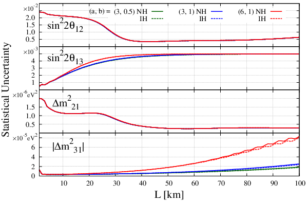
We find

	$\displaystyle\delta\sin^{2}2\theta_{12}\sim$	$\displaystyle 4\times 10^{-3}\,(0.5\%),$		(4.1a)
	$\displaystyle\delta\Delta m^{2}_{21}\sim$	$\displaystyle 3\times 10^{-7}{\rm eV^{2}}\,(0.4\%),$		(4.1b)
	$\displaystyle\delta|\Delta m^{2}_{31}|\sim$	$\displaystyle 7\times 10^{-6}{\rm eV^{2}}\,(0.3\%),$		(4.1c)

with the energy resolution of $(a,b)=(3,0.5)\%$ at $L=50$ km; the percentage values in the parentheses denote the relative accuracy of the measurement. Those uncertainties are almost independent of the mass hierarchy and of the energy resolution, with the only exception of the $|\Delta m^{2}_{31}|$ uncertainty for which the larger resolution results in the larger uncertainty: $|\Delta m^{2}_{31}|\sim 8\times 10^{-6}{\rm eV}^{2}$ for the resolution $(a,b)=(3,1)\%$ and $1.8\times 10^{-5}{\rm eV}^{2}$ for $(a,b)=(6,1)\%$ at $L=50$ km. The uncertainties of $\sin^{2}2\theta_{12}$ and $\Delta m^{2}_{21}$ show the rapid reduction after $L=20$ km and stabilize for $L>40$ km. This is because the normalization and shape of the slowly varying oscillation pattern in Fig. 1 determine $\sin^{2}2\theta_{12}$ and $\Delta m^{2}_{21}$, respectively, which is almost independent of the energy resolution. On the other hand, $\sin^{2}2\theta_{13}$ and $|\Delta m^{2}_{31}|$ are measured most accurately around $L\sim 1$ km, which motivated the first round of the reactor antineutrino oscillation experiments such as Daya Bay [1, *An:2012bu], RENO [3] and Double Chooz [55]. The uncertainty of $\sin^{2}2\theta_{13}$ quickly grows to the Daya Bay expectation of 5% [59], which is implemented as the input in this analysis, at $L>30$ km. Somewhat surprisingly, the uncertainty of $|\Delta m^{2}_{31}|$ remains small at the level of $1\times 10^{-6}{\rm eV}^{2}$ up to $L\sim 60$ km when energy resolution is $3\%/\sqrt{E/{\rm MeV}}$ or better. We find that this is because the rapid oscillation pattern due to $|\Delta m^{2}_{31}|$ can be resolved even after the smearing in the observed energy as can be seen in Fig. 3. With better energy resolution, more oscillation patterns are recognized and higher accuracy of the $|\Delta m^{2}_{31}|$ measurement can be achieved.

We have discussed the sensitivity for the mass hierarchy determination by evaluating the minimum of $\Delta\chi^{2}$ in eq. (3.6) without taking account of statistical fluctuations in the data. In general, fluctuations can be included by simulating many experiments repeatedly; for example, see refs. [44, 47, 48]. However, it requires time-consuming simulations. Here, we introduce a more efficient way to estimate effects of statistical fluctuations on the sensitivity.

The $\chi^{2}$ function (3.1) can be written as

$\displaystyle\chi^{2}=$

$\displaystyle\sum_{i=1}^{\rm nbin}\left(\frac{N_{i}^{\rm fit}-N^{\rm data}_{i}}{\sqrt{N_{i}^{\rm data}}}\right)^{2}+\sum_{i=1}^{\rm nparam}\left(\frac{X_{i}-X^{\rm input}_{i}}{\delta X_{i}}\right)^{2},$

(5.1)

where $N^{\rm fit}_{i}$ and $N^{\rm data}_{i}$ are the predicted and observed event numbers in the $i_{\rm th}$ bin, and “nbin” and “nparam” are the numbers of bins and parameters used in the $\chi^{2}$ fitting, respectively. The second term gives the contributions from the external constraints on the model parameters and systematic errors, see eqs. (3.2) and (3.3).

We first expand the theoretical prediction $N^{\rm fit}_{i}$ as

$$N^{\rm fit}_{i}\approx n^{(0)}_{i}+\sum_{j}A_{ij}\Delta X_{j}\,.$$

(5.2)

keeping only the terms linear in $\Delta X_{j}$. Here $n^{(0)}_{i}=N^{\rm fit}_{i}|_{X=X^{(0)}}$ are the predicted event numbers where the parameters are set at reference values $X_{j}=X^{(0)}_{j}$; $\Delta X_{j}$ are the deviations of parameters from their reference values, $\Delta X_{j}\equiv X_{j}-X^{(0)}_{j}$; and $A_{ij}$ are the corresponding derivatives, $A_{ij}=\partial N^{\rm fit}_{i}/\partial X_{j}|_{X=X^{(0)}}$. This linear expansion gives the true $\chi^{2}_{\rm min}$ for both the true and wrong mass-hierarchy assumptions after a few iterations of minimization since all the neutrino parameters used in this analysis have been well constrained by previous experiments.

For convenience, we rewrite eq. (5.1) in the matrix form,

	$$\chi^{2}=(\tilde{n}^{(0)}+\tilde{A}\Delta X-\tilde{N}^{\rm data})^{T}\Sigma^{-1}(\tilde{n}^{(0)}+\tilde{A}\Delta X-\tilde{N}^{\rm data})\,,$$		(5.3a)
with the diagonal $({\rm nbin}+{\rm nparam})\times({\rm nbin}+{\rm nparam})$ matrix
	$$\Sigma_{ij}=\delta_{ij}(\delta\tilde{N}_{i})^{2},$$		(5.3b)

where

		$\displaystyle\tilde{n}^{(0)}_{i}=n^{(0)}_{i}$
		$\displaystyle\tilde{A}_{ik}=A_{ik}$
		$\displaystyle\tilde{N}^{\rm data}_{i}=N^{\rm data}_{i}$
		$\displaystyle\delta\tilde{N}_{i}=\sqrt{N_{i}^{\rm data}}$			(5.4a)
for $1\leq i\leq{\rm nbin}$ and $1\leq k\leq{\rm nparam}$, and
		$\displaystyle\tilde{n}^{(0)}_{l}=X^{(0)}_{l-{\rm nbin}}$
		$\displaystyle\tilde{A}_{lk}=\delta_{l-{\rm nbin},\,k}$
		$\displaystyle\tilde{N}^{\rm data}_{l}=X^{\rm input}_{l-{\rm nbin}}$
		$\displaystyle\delta\tilde{N}_{l}=\delta X_{l-{\rm nbin}}$			(5.4b)

for (${\rm nbin}+1)\leq l\leq({\rm nbin}+{\rm nparam}$). For a given set of data $\left\{N_{i}^{\rm data}\right\}(1\leq i\leq{\rm nbin})$, we find a minimum of eq. (5.3a) by varying the parameters $\Delta X_{k}\,(1\leq k\leq{\rm nparam})$. The extremum condition reads

$$\frac{\partial\chi^{2}}{\partial\Delta X}=2\tilde{A}^{T}\Sigma^{-1}(\tilde{n}^{(0)}+\tilde{A}\Delta X-\tilde{N}^{\rm data})=0\,,$$

(5.5)

which can be solved as

$$\Delta X_{\rm best}=-(\tilde{A}^{T}\Sigma^{-1}\tilde{A})^{-1}\tilde{A}^{T}\Sigma^{-1}(\tilde{n}^{(0)}-\tilde{N}^{\rm data})\,.$$

(5.6)

The minimum $\chi^{2}$ is estimated with this best-fit $\Delta X$ as

	$\displaystyle\chi^{2}_{\rm min}\left(N^{\rm data}\right)$	$\displaystyle=$	$\displaystyle(\tilde{n}^{(0)}-\tilde{N}^{\rm data})^{T}[I-\tilde{A}(\tilde{A}^{T}\Sigma^{-1}\tilde{A})^{-1}\tilde{A}^{T}\Sigma^{-1}]^{T}\Sigma^{-1}$		(5.7)
			$\displaystyle[I-\tilde{A}(\tilde{A}^{T}\Sigma^{-1}\tilde{A})^{-1}\tilde{A}^{T}\Sigma^{-1}](\tilde{n}^{(0)}-\tilde{N}^{\rm data}).$

Note that the event number dependence of $\chi^{2}_{\rm min}$ comes from the event number difference, ($n^{(0)}-N^{\rm data}$), and $\Sigma_{ij}$. The true $\chi^{2}_{\rm min}$ is found by iterating the procedure a few times.

Due to fluctuation, $N^{\rm data}_{i}$ may deviate from their mean values $\overline{N}_{i}$, and the $(\Delta\chi^{2})_{\rm min}$ has the statistical uncertainty. It is plausibly assumed that these fluctuation of $N^{\rm data}_{i}$ follow the Gaussian distributions with the variance $\sqrt{\overline{N}_{i}}$. The uncertainty of the $(\Delta\chi^{2})_{\rm min}$ can then be estimated as

$\displaystyle\delta\left\{(\Delta\chi^{2})_{\rm min}\right\}=$

$\displaystyle\sqrt{\sum_{i=1}^{\rm nbin}\left(\left.\frac{\partial(\Delta\chi^{2})_{\rm min}}{\partial N^{\rm data}_{i}}\right|_{N^{\rm data}=\overline{N}}\,\sqrt{\overline{N}_{i}}\right)^{2}}.$

(5.8)

This can be calculated from eq. (5.7) analytically. Therefore, we can readily estimate the uncertainty of the $(\Delta\chi^{2})_{\rm min}$, once we find a set of $X^{(0)}_{i}$ which gives the true $\chi^{2}_{\rm min}$.

This uncertainty is actually closely related to the mean of the $(\Delta\chi^{2})_{\rm min}$,

$$\overline{(\Delta\chi^{2})_{\rm min}}=\left.(\Delta\chi^{2})_{\rm min}\right|_{N^{\rm data}=\overline{N}},$$

(5.9)

as

$$\delta\left\{(\Delta\chi^{2})_{\rm min}\right\}\sim 2\sqrt{\overline{(\Delta\chi^{2})_{\rm min}}}.$$

(5.10)

It may be explained as follows. The derivative of $(\Delta\chi^{2})_{\rm min}$ with respect to $N^{\rm data}_{i}$ in eq. (5.8) consists of two parts: the linear terms and the quadratic terms of the event number difference $\left(n^{(0)}_{i}-N^{\rm data}_{i}\right)$. Since this difference is tiny with respect to the event number itself, we can just keep the linear terms and obtain the relation (5.10). The same result was obtained by the authors of ref. [50] in a different approach.

We can now estimate the probability of an experiment to determine the right mass hierarchy. It is plausible to assume that $(\Delta\chi^{2})_{\rm min}$ corresponding to the right mass-hierarchy determination follows the normal distribution with the mean $\overline{(\Delta\chi^{2})_{\rm min}}$ and the standard deviation $\delta\left\{(\Delta\chi^{2})_{\rm min}\right\}$ [50]. The sensitivity corresponding to a given $(\Delta\chi^{2})_{\rm min}$ is then evaluated as ${\rm erf}\left(\frac{1}{\sqrt{2}}\sqrt{(\Delta\chi^{2})_{\rm min}}\right)$ with the Gauss error function

$${\rm erf}\left(\frac{x}{\sqrt{2}}\right)\equiv\int^{x}_{-x}dy\,\frac{1}{\sqrt{2\pi}}e^{-\frac{y^{2}}{2}}.$$

(5.11)

The probability for an experiment to determine the right mass hierarchy is then calculated as

$\displaystyle P$

$\displaystyle=\int^{\infty}_{0}dx\,N\left(x;\overline{(\Delta\chi^{2})_{\rm min}},\,\delta\left\{(\Delta\chi^{2})_{\rm min}\right\}\right){\rm erf}\left(\frac{\sqrt{x}}{\sqrt{2}}\right),$

(5.12)

where $N(x;\mu,\sigma)$ is the normal distribution function

$$N(x;\mu,\sigma)\equiv\frac{1}{\sqrt{2\pi}\sigma}\exp\left\{-\frac{(x-\mu)^{2}}{2\sigma^{2}}\right\}.$$

(5.13)

Note that the normal distribution function does not add up to unity over the integration interval, $(0,\infty)$, since there is also the possibility that the wrong mass hierarchy is chosen.

To check the validity of our method for estimating the uncertainty of $(\Delta\chi^{2})_{\rm min}$, we evaluate the probability, eq. (5.12), with a Monte-Carlo (MC) method as well. We generate 1,000 pseudo experiments each for several energy resolutions and experimental exposures. From the obtained 1,000 $(\Delta\chi^{2})_{\rm min}$, we estimate the mean and the variance of the $(\Delta\chi^{2})_{\rm min}$ and calculate the probability using eq. (5.12).

We show our naive expectation for the probability of an experiment to determine the right mass hierarchy, subtracted from unity, as a function of the $\sqrt{\overline{(\Delta\chi^{2})_{\rm min}}}$ in Fig. 9 (the solid curve).

Although the curve is obtained for the NH case with the $(a,b)=(2,0.5)\%$ energy resolution, it depends neither on the mass hierarchy nor on the energy resolution. The dashed curve shows the simple Gaussian interpretation of the $\overline{(\Delta\chi^{2})_{\rm min}}$ as a reference. Circle and rectangular points show the expected sensitivity obtained by the MC method for experiments with the energy resolution of $(2,0.5)\%$ and $(3,0.75)\%$, respectively. The experimental exposures are taken to be ${\rm 20\,GW_{th}}$$\cdot$5kt (12% free-proton weight fraction)$\cdot$5yrs $\times 1,\times 4$ and $\times 9$ for the $(2,0.5)\%$ resolution case, while they are $\times 1,\times 4,\times 9,\times 16$ and $\times 25$ for the $(3,0.75)\%$ resolution case. These points agree with the expected-sensitivity curve obtained with our analytical method, demonstrating the validity of our approach. We have checked that all the central values of the MC simulation results lie on the solid curve when we increase the number of pseudo-experiments to $10,000$.

As an illustration, let us consider an experiment with the energy resolution of $(a,b)=(2,0.5)\%$ and ${\rm 20\,GW_{th}}$$\cdot$5kt (12% free-proton weight fraction)$\cdot$5yrs  exposure. $(\Delta\chi^{2})_{\rm min}\simeq 11.8$ for NH and $11.6$ for IH from Fig. 7, and the solid curve in Fig. 9 tells that the experiment is expected to determine the right mass hierarchy with $\sim 94\%$ probability for both hierarchies.

The authors of ref. [48] considered the probability of determining the right hierarchy against the wrong hierarchy. They estimated the fluctuation of the sensitivity for mass hierarchy determination by simulating many experiments. They found the probability of 98.9% with the energy resolution of $(a,b)=(2.6,1)\%$ at the baseline length of 60 km and with five times more events ($10^{5}$ events) than our default setting, assuming $\sin^{2}2\theta_{13}=0.092\pm 0.017$. We find $(\Delta\chi^{2})_{\rm min}\simeq 21$ for their setting, giving $\sim 98.7\%$ probability with eq. (5.12), showing the good agreement with their result. On the other hand, authors of ref. [47, 44] considered the probability to determine the mass hierarchy correctly, by using the Fourier analysis. Although the definition of the probability is not stated clearly in the references, the probability may correspond to our eq. (5.12) where the error function ${\rm erf}(\sqrt{x}/\sqrt{2})$ is replaced by unity. They reported $\sim 90\%$ and $93.4\%$ probabilities for experiments with $(a,b)=(3,0)\%$ energy resolution at the baseline length of 58 km and with 25 and 2.5 times more events ($5\times 10^{5}$ and $5\times 10^{4}$ events) than our default setting, assuming $\sin^{2}2\theta_{13}=0.02$ and 0.092, respectively. For those settings, we find $(\Delta\chi^{2})_{\rm min}\simeq 5.7$ and 11.7, giving the probabilities of $\sim 83\%$ and $\sim 93.6\%$ with eq. (5.12), respectively. Somewhat smaller probability of our estimate $\sim 83\%$ may reflect the factor ${\rm erf}(\sqrt{x}/\sqrt{2})<1$ in eq. (5.12), whose effect can be significant when $(\Delta\chi^{2})_{\rm min}$ is not large. Another possible reason is that only one set of parameter values was studied in their analysis without marginalizing the probabilities as pointed out in ref. [48].

In this paper we have investigated the sensitivity of medium baseline reactor electron-antineutrino oscillation experiments for determining the neutrino mass hierarchy by performing the standard $\chi^{2}$ analysis.

We carefully study the impacts of the energy resolution $(\delta E/E)^{2}=\left(a/\sqrt{E/{\rm MeV}}\right)^{2}+b^{2}$ and find that the sensitivity and the optimal baseline length, which maximizes the mass hierarchy resolving power of the experiment, strongly depend on it. The optimal baseline length is found to depend slightly on the energy resolution, preferring the length slightly shorter than 50 km for the energy resolution of $(a,b)=(3,0.75)\%,(3,1)\%,(2,0.75)\%$ and $(2,1)\%$. At the optimal baseline length, the energy resolution better than the $3\%/\sqrt{E/{\rm MeV}}$ level is needed to determine the neutrino mass hierarchy pattern. $3\sigma$ determination of the mass hierarchy is possible for an experiment with ${\rm 20\,GW_{th}}$$\cdot$5kt (12% free-proton weight fraction)$\cdot$5yrs  exposure if an energy resolution of $(a,b)=(2,0.75)\%$ is achieved, while a factor of three larger or longer experiment is needed to achieve the same goal for the energy resolution of $(a,b)=(3,0.75)\%$.

It is also found that this experiment can measure the neutrino parameters, $\sin^{2}2\theta_{12}$, $\Delta m^{2}_{21}$ and $|\Delta m^{2}_{31}|$, very accurately as shown in (4.1) for an experiment of ${\rm 20\,GW_{th}}$$\cdot$5kt (12% free-proton weight fraction)$\cdot$5yrs  at $L\sim 50$ km.

The statistical uncertainty of the $(\Delta\chi^{2})_{\rm min}$ is then estimated with an efficient analytic method. Applying this, we evaluate and discuss the expected sensitivity for determining the right mass hierarchy. This method is generic and can be applied straightforwardly to other experiments, especially to those where MC methods cost much.

References

- [1] F. P. An et al. (Daya Bay Collaboration), Phys.Rev.Lett. 108 (2012a) 171803 [arXiv:1203.1669].
- [2] F. P. An et al. (Daya Bay Collaboration), arXiv:1210.6327 (2012b).
- [3] J. K. Ahn et al. (RENO collaboration), Phys.Rev.Lett. 108 (2012) 191802 [arXiv:1204.0626].
- [4] H. Minakata and H. Nunokawa, JHEP 0110 (2001a) 001 [arXiv:hep-ph/0108085].
- [5] V. Barger, D. Marfatia and K. Whisnant, Phys.Rev. D65 (2002a) 073023 [arXiv:hep-ph/0112119].
- [6] P. Huber, M. Lindner and W. Winter, Nucl.Phys. B645 (2002) 3 [arXiv:hep-ph/0204352].
- [7] H. Minakata, H. Nunokawa and S. J. Parke, Phys.Rev. D68 (2003) 013010 [arXiv:hep-ph/0301210].
- [8] M. Blennow and T. Schwetz, JHEP 1208 (2012a) 058 [arXiv:1203.3388].
- [9] S. Dusini, A. Longhin, M. Mezzetto, L. Patrizii, M. Sioli, G. Sirri and F. Terranova, arXiv:1209.5010 (2012).
- [10] H.-s. Chen et al. (VLBL Study Group H2B-1), arXiv:hep-ph/0104266 (2001).
- [11] M. Aoki, K. Hagiwara, Y. Hayato, T. Kobayashi, T. Nakaya, K. Nishikawa and N. Okamura, Phys.Rev. D67 (2003) 093004 [arXiv:hep-ph/0112338].
- [12] M. Ishitsuka, T. Kajita, H. Minakata and H. Nunokawa, Phys.Rev. D72 (2005) 033003 [arXiv:hep-ph/0504026].
- [13] K. Hagiwara, N. Okamura and K.-i. Senda, Phys.Lett. B637 (2006) 266 [arXiv:hep-ph/0504061].
- [14] K. Hagiwara, N. Okamura and K.-i. Senda, Phys.Rev. D76 (2007) 093002 [arXiv:hep-ph/0607255].
- [15] T. Kajita, H. Minakata, S. Nakayama and H. Nunokawa, Phys.Rev. D75 (2007) 013006 [arXiv:hep-ph/0609286].
- [16] K. Hagiwara and N. Okamura, JHEP 0801 (2008) 022 [arXiv:hep-ph/0611058].
- [17] K. Hagiwara and N. Okamura, JHEP 0907 (2009) 031 [arXiv:0901.1517].
- [18] K. Hagiwara, T. Kiwanami, N. Okamura and K.-i. Senda, arXiv:1209.2763 (2012).
- [19] S. Palomares-Ruiz and S. T. Petcov, Nucl.Phys. B712 (2005) 392 [arXiv:hep-ph/0406096].
- [20] R. Gandhi, P. Ghoshal, S. Goswami, P. Mehta and S. Uma Sankar, arXiv:hep-ph/0506145 (2005).
- [21] S. T. Petcov and T. Schwetz, Nucl.Phys. B740 (2006) 1 [arXiv:hep-ph/0511277].
- [22] M. Blennow and T. Schwetz, JHEP 1208 (2012b) 058 [arXiv:1203.3388].
- [23] A. S. Dighe and A. Y. Smirnov, Phys.Rev. D62 (2000) 033007 [arXiv:hep-ph/9907423].
- [24] H. Minakata and H. Nunokawa, Phys.Lett. B504 (2001b) 301 [arXiv:hep-ph/0010240].
- [25] V. Barger, D. Marfatia and B. P. Wood, Phys.Lett. B532 (2002b) 19 [arXiv:hep-ph/0202158].
- [26] C. Lunardini and A. Y. Smirnov, JCAP 0306 (2003) 009 [arXiv:hep-ph/0302033].
- [27] A. S. Dighe, M. T. Keil and G. G. Raffelt, JCAP 0306 (2003a) 005 [arXiv:hep-ph/0303210].
- [28] A. S. Dighe, M. T. Keil and G. G. Raffelt, JCAP 0306 (2003b) 006 [arXiv:hep-ph/0304150].
- [29] V. Barger, P. Huber and D. Marfatia, Phys.Lett. B617 (2005) 167 [arXiv:hep-ph/0501184].
- [30] S. M. Bilenky, C. Giunti, W. Grimus, B. Kayser and S. T. Petcov, Phys.Lett. B465 (1999) 193 [arXiv:hep-ph/9907234].
- [31] H. V. Klapdor-Kleingrothaus, H. Pas and A. Y. Smirnov, Phys.Rev. D63 (2001) 073005 [arXiv:hep-ph/0003219].
- [32] S. M. Bilenky, S. Pascoli and S. T. Petcov, Phys.Rev. D64 (2001) 053010 [arXiv:hep-ph/0102265].
- [33] S. Pascoli, S. T. Petcov and L. Wolfenstein, Phys.Lett. B524 (2002) 319 [arXiv:hep-ph/0110287].
- [34] F. Feruglio, A. Strumia and F. Vissani, Nucl.Phys. B637 (2002) 345 [arXiv:hep-ph/0201291].
- [35] S. Pascoli and S. T. Petcov, Phys.Lett. B544 (2002) 239 [arXiv:hep-ph/0205022].
- [36] S. Pascoli, S. T. Petcov and W. Rodejohann, Phys.Lett. B558 (2003) 141 [arXiv:hep-ph/0212113].
- [37] S. T. Petcov, Phys.Scripta T121 (2005) 94 [arXiv:hep-ph/0504166].
- [38] A. Dueck, W. Rodejohann and K. Zuber, Phys.Rev. D83 (2011) 113010 [arXiv:1103.4152].
- [39] S. T. Petcov and M. Piai, Phys.Lett. B533 (2002) 94 [arXiv:hep-ph/0112074].
- [40] S. Choubey, S. T. Petcov and M. Piai, Phys.Rev. D68 (2003) 113006 [arXiv:hep-ph/0306017].
- [41] J. Learned, S. T. Dye, S. Pakvasa and R. C. Svoboda, Phys.Rev. D78 (2008) 071302 [arXiv:hep-ex/0612022].
- [42] L. Zhan, Y. Wang, J. Cao and L. Wen, Phys.Rev. D78 (2008) 111103 [arXiv:0807.3203].
- [43] M. Batygov, S. Dye, J. Learned, S. Matsuno, S. Pakvasa and G. Varner, arXiv:0810.2580 (2008).
- [44] L. Zhan, Y. Wang, J. Cao and L. Wen, Phys.Rev. D79 (2009) 073007 [arXiv:0901.2976].
- [45] P. Ghoshal and S. T. Petcov, JHEP 1103 (2011) 058 [arXiv:1011.1646].
- [46] E. Ciuffoli, J. Evslin and X. Zhang, arXiv:1208.1991 (2012a).
- [47] E. Ciuffoli, J. Evslin and X. Zhang, arXiv:1209.2227 (2012b).
- [48] X. Qian, D. A. Dwyer, R. D. McKeown, P. Vogel, W. Wang and C. Zhang, arXiv:1208.1551 (2012a).
- [49] P. Ghoshal and S. T. Petcov, arXiv:1208.6473 (2012).
- [50] X. Qian, A. Tan, W. Wang, J. J. Ling, R. D. McKeown and C. Zhang, arXiv:1210.3651 (2012b).
- [51] C. Bemporad, G. Gratta and P. Vogel, Rev.Mod.Phys. 74 (2002) 297 [arXiv:hep-ph/0107277].
- [52] P. Vogel and J. Engel, Phys.Rev. D39 (1989) 3378.
- [53] P. Huber and T. Schwetz, Phys.Rev. D70 (2004) 053011 [arXiv:hep-ph/0407026].
- [54] K. Hagiwara, N. Okamura and K. Senda, JHEP 1109 (2011) 082 [arXiv:1107.5857].
- [55] Y. Abe et al. (DOUBLE-CHOOZ Collaboration), Phys.Rev.Lett. 108 (2012) 131801 [arXiv:1112.6353].
- [56] P. Vogel and J. F. Beacom, Phys.Rev. D60 (1999) 053003 [arXiv:hep-ph/9903554].
- [57] X. Qian and Y. Wang, private communication.
- [58] J. Beringer et al. (Particle Data Group), Phys.Rev. D86 (2012) 010001.
- [59] J. Cao, talk at ICHEP2012 in Melbourne.