Holographic RG flows in six dimensional F(4) gauged supergravity

Preprint: arXiv: 1210.8064

Parinya Karndumri Affiliation: String Theory and Supergravity Group, Department of Physics, Faculty of Science, Chulalongkorn University, 254 Phayathai Road, Pathumwan, Bangkok 10330, Thailand Affiliation: Thailand Center of Excellence in Physics, CHE, Ministry of Education, 319 Dusit, Bangkok 10400, Thailand Email: parinya.ka@hotmail.com Affiliation: E-mail:

Abstract:

We study critical points of $F(4)$ gauged supergravity in six dimensions coupled to three vector multiplets. Scalar fields are described by $\mathbb{R}^{+}\times\frac{SO(4,3)}{SO(4)\times SO(3)}$ coset space, and the gauge group is given by $SO(3)_{R}\times SO(3)$ with $SO(3)_{R}$ being the R-symmetry. The maximally supersymmetric critical point with all scalars vanishing preserves the full $SO(3)_{R}\times SO(3)$ symmetry. This is dual to a superconformal field theories (SCFT₅) arising from a near horizon geometry of the D4-D8 brane system in type I^′ theory with an enhanced global symmetry $E_{1}\sim SU(2)$ . Apart from this trivial critical point, we identify a new supersymmetric critical point preserving the full supersymmetry with the $SO(3)_{R}\times SO(3)$ symmetry broken to its diagonal subgroup. This critical point should correspond to a new SCFT in five dimensions. We study an RG flow solution interpolating between the SCFT with $E_{1}$ symmetry and the new supersymmetric critical point. The flow describes a supersymmetric deformation driven by a vacuum expectation value of relevant operators of dimension $3$ . We identify the dual operators with the mass terms for hypermultiplet scalars in the dual field theory. The solution provides an example of analytic supersymmetric RG flows in AdS₆/CFT₅ correspondence.

Keywords:

AdS-CFT correspondence, Gauge/Gravity Correspondence and Supergravity Models

1 Introduction

The study of holographic renormalization group (RG) flow is one of the most important applications of the AdS/CFT correspondence [1]. Soon after the original proposal of the correspondence, many works considering RG flows in five dimensional gauged supergravity have been done, see for example [2], [3] and [4]. These results describe various perturbations of $N=4$ SYM in four dimensions. Since the AdS/CFT correspondence has been extended to other dimensions not only for the duality between an $AdS_{5}$ supergravity and a CFT₄ [5, 6, 7, 8, 9], it is interesting to study holographic RG flows in these extensions as well. Until now, a lot of works on holographic RG flows in three and four dimensional gauged supergravities have appeared, see for example [10], [11], [12], [13] and [14].
On the other hand, a study of AdS₆/CFT₅ correspondence has not been explored in details although some works in this direction can be found in [7] and [15], see also [16] for a more recent result. To the best of the author’s knowledge, only one holographic RG flow solution, studied in [17], in AdS₆/CFT₅ correspondence has been studied so far. This work will provide another example which is related to a deformation of five dimensional $N=2$ SYM at a conformal fixed point with enhanced global symmetry $SU(2)$ .
The starting point is the $F(4)$ gauged supergravity in six dimensions with $N=(1,1)$ supersymmetries. The pure $F(4)$ gauged supergravity has been constructed in [18]. It has been known since its first construction that the scalar potential of the pure $F(4)$ gauged supergravity admits two critical points [18]. One of them is maximally supersymmetric, and the other one breaks all supersymmetries. The latter is however stable and should correspond to a non-supersymmetric conformal field theory according to the general principle of the AdS/CFT correspondence. A numerical RG flow solution interpolating between these two critical points has been given in [17]. This pure $F(4)$ gauged supergravity has also been studied in the context of holography in [19] in which RG flows between a UV CFT₅ and an IR CFT₃ or CFT₂ have been given.
In this work, we consider an RG flow in AdS₆/CFT₅ correspondence from matter coupled $F(4)$ gauged supergravity constructed in [20] and [21]. The dual CFT’s with $N=2$ supersymmetry are fixed points of the $N=2$ $USp(2k)$ SYM theory describing the worldvolume theory of D4-branes [22], see also [23]. The fixed points corresponding to interacting CFT’s arise in an infinite coupling limit. In term of brane configurations, they can be described as near horizon geometries of the D4-D8 brane system in type I^′ theory [24]. The configuration should also be obtained in massive type IIA theory where the D8-branes are known to exist [15]. At the fixed points, the $SO(2N_{f})\times U(1)$ global symmetry gets enhanced to $E_{N_{f}+1}$ , $N_{f}=0,\ldots,7$ with $E_{1}=SU(2)$ , $E_{2}=SU(2)\times U(1)$ , $E_{3}=SU(3)\times SU(2)$ , $E_{4}=SU(5)$ and $E_{5}=SO(10)$ [22]. $E_{6,7,8}$ are the usual exceptional groups. $N_{f}$ denotes the number of flavor hypermultiplets or equivalently the number of D8-branes. The extension to theories with global symmetry $\tilde{E}_{1}=U(1)$ and $E_{0}=\mathbf{I}$ (no global symmetry) has been studied in [25]. The matter coupled $F(4)$ gauged supergravity whose scalars paramatrized by $\mathbb{R}^{+}\times\frac{SO(4,n)}{SO(4)\times SO(n)}$ coset space can give rise to gravity duals of these 5-dimensional CFTs with enhanced global symmetry by gauging the $SU(2)_{R}\times G$ subgroup of $SO(4)\times SO(n)$ . $n$ denotes the number of matter multiplets, vector multiplets in this case. $SU(2)_{R}$ is the R-symmetry given by the diagonal subgroup of $SU(2)\times SU(2)\sim SO(4)$ , and $G$ is identified with the flavor symmetry $E_{N_{f}+1}$ with $n=\textrm{dim}\,G$ .
The full symmetry at the fixed points is given by $F(4)\times G$ . The $F(4)$ is the superconformal group containing $SU(2)_{R}\times SO(5,2)$ as its bosonic subgroup. The correspondence between $F(4)$ gauged supergravity and these five dimensional CFTs has been discussed in [15], and some relations between supergravity fields with the global symmetry $G$ being $E_{7}$ and their dual operators have been identified. These relations have been verified to be consistent with the spectrum of the matter coupled $F(4)$ gauged supergravity theory in [20].
We will consider a simple case of the matter coupled $F(4)$ gauged supergravity in which there are three matter (vector) multiplets. This case corresponds to $N_{f}=0$ or, equivalently, no D8-branes present. We will study the scalar potential of the theory and identify some of the critical points. This gives the first non-trivial critical point in matter coupled $F(4)$ gauged supergravity and describes a new supersymmetric fixed point of the dual field theory in five dimensions. We then compute the full scalar mass spectrum at the critical point which will give information on dimensions of the dual operators. We will also study an RG flow solution corresponding to a supersymmetric deformation of the UV $N=2$ CFT with global $SU(2)$ symmetry by a vacuum expectation value of dimension-3 operators.
The paper is organized as follow. In section 2, we give some formulae in the matter coupled $F(4)$ gauged supergravity which forms a framework of the whole paper. We will give our notations and conventions which are slightly different from [20] and [21]. In section 3, we study the scalar potential and identify new critical points of the matter coupled $F(4)$ gauged supergravity. We will also give scalar mass spectra at each critical point. An RG flow solution connecting the trivial critical point with maximal supersymmetry and a new supersymmetric critical point with the same amount of supersymmetry will be given in section 4. Finally, we give our conclusions and comments in section 5.

2 Matter coupled $F(4)$ gauged supergravity

In this section, we review the construction and relevant formulae for the matter coupled $F(4)$ gauged supergravity. Although we will work with the metric signature $(-+++++)$ , most of the notations and conventions used in this work will be closely parallel to those given in [20] and [21]. We refer the reader to these references for a beautiful geometric construction. Some gaugings of this theory can be obtained from a truncation of the maximal gauged supergravity in six dimensions. Moreover, these gaugings can be described in an $O(1,1)\times SO(4,n)$ covariant form using the embedding tensor formalism [26]. However, in this paper, we will restrict ourselves to the construction of [20] and [21].

2.1 General matter coupled $F(4)$ gauged supergravity

The $F(4)$ supergravity is a half maximal, $N=(1,1)$ , supergravity in six dimensions. The field content of the supergravity multiplet is given by

\left(e^{a}_{\mu},\psi^{A}_{\mu},A^{\alpha}_{\mu},B_{\mu\nu},\chi^{A},\sigma\right)

where $e^{a}_{\mu}$ , $\chi^{A}$ and $\psi^{A}_{\mu}$ denote the graviton, the spin $\frac{1}{2}$ field and the gravitino, respectively. Space-time and tangent space indices are denoted by $\mu,\nu,\ldots$ and $a,b,\ldots$ . Both $\chi^{A}$ and $\psi^{A}_{\mu}$ are the eight-component pseudo-Majorana spinor with indices $A,B=1,2$ referring to the fundamental representation of the $SU(2)_{R}$ R-symmetry. The remaining fields are given by the dilaton $\sigma$ , four vectors $A^{\alpha}_{\mu},\,\alpha=0,1,2,3$ , and a two-form field $B_{\mu\nu}$ . As in [20], it is more convenient in the gauged theory to decompose the $\alpha$ index into $\alpha=(0,r)$ in which $r=1,2,3$ .
The matter field in the $N=(1,1)$ theory is given by the vector multiplet whose field content is

(A_{\mu},\lambda_{A},\phi^{\alpha}).

We will label each matter multiplet by an index $I=1,\ldots,n$ . The $4n$ scalars $\phi^{\alpha I}$ are described by a symmetric space $SO(4,n)/SO(4)\times SO(n)$ . Furthermore, the dilaton $\sigma$ can be regarded as living in the coset space $\mathbb{R}^{+}\sim O(1,1)$ which is the duality group of the pure supergravity theory. Together, the $4n+1$ scalars of the matter coupled theory live in the coset space

\mathbb{R}^{+}\times\frac{SO(4,n)}{SO(4)\times SO(n)},

(1)

and the global symmetry is given by $O(1,1)\times SO(4,n)$ . The $SU(2)_{R}$ R-symmetry is the diagonal subgroup of $SU(2)\times SU(2)\sim SO(4)\subset SO(4)\times SO(n)$ .
$O(1,1)$ can be parametrized by $e^{\sigma}$ while the $SO(4,n)/SO(4)\times SO(n)$ coset will be parametrized by the coset representative $L^{\Lambda}_{\phantom{as}\Sigma}$ , $\Lambda,\Sigma=0,\ldots,3+n$ . It is also convenient to split the $L^{\Lambda}_{\phantom{as}\Sigma}$ into $(L^{\Lambda}_{\phantom{as}\alpha},L^{\Lambda}_{\phantom{as}I})$ and further to $(L^{\Lambda}_{\phantom{as}0},L^{\Lambda}_{\phantom{as}r},L^{\Lambda}_{\phantom{as}I})$ . The composite connections $Q$ and the vielbein of the coset $P$ are defined schematically via

L^{-1}dL=Q+P\,.

(2)

We now come to gaugings of the matter coupled theory and will restrict ourselves to compact gaugings. The gauge group is a subgroup of $SO(4)\times SO(n)\subset SO(4,n)$ . In the pure gauged supergravity, the gauge group is given by $SU(2)_{R}$ . In the matter coupled case, we consider the gauge group of the form $SU(2)_{R}\times G$ with $\textrm{dim}\,G=n$ . The restriction $\textrm{dim}\,G=n$ comes from the fact that there are only $n$ vector multiplets, or equivalently the maximum number of the gauge fields for the gauge group $G$ is given by $n$ . We will denote the structure constant of the full gauge group $SU(2)_{R}\times G$ by $f^{\Lambda}_{\phantom{as}\Pi\Sigma}$ which can be split into $\epsilon_{rst}$ and $C_{IJK}$ for $SU(2)_{R}$ and $G$ , respectively.
As usual, the gauging is implemented by covariantizing all the derivatives, and to restore the supersymmetry, fermionic mass-like terms and a scalar potential are introduced. We only give some needed information to our study of the vacua and RG flows and refer the reader to [20] and [21] for more details. Moreover, the supersymmetry transformations of fermions are also modified by some shifts at first order in the gauge couplings. The direct product structure of the gauge group $SU(2)_{R}\times G$ leads to two coupling constants $g_{1}$ and $g_{2}$ . As has been shown in [21], without the mass parameter $m$ of the two-form field the maximally supersymmetric $AdS_{6}$ vacuum does not exist. Therefore, only the $m\neq 0$ case is relevant for the present work.
The bosonic Lagrangian under consideration here consists of the metric and scalars [21]

\mathcal{L}=\frac{1}{4}eR-e\partial_{\mu}\sigma\partial^{\mu}\sigma-\frac{1}{4}eP_{I\alpha\mu}P^{I\alpha\mu}-eV

(3)

where $e=\sqrt{-g}$ . The $\phi^{I\alpha}$ kinetic term is written in term of $P^{I\alpha}_{\mu}=P^{I\alpha}_{i}\partial_{\mu}\phi^{i}$ , $i=1,\ldots,4n$ . The scalar potential is given by [21]

	$\displaystyle V$	$\displaystyle=$	$\displaystyle-e^{2\sigma}\left[\frac{1}{36}A^{2}+\frac{1}{4}B^{i}B_{i}+\frac{1}{4}\left(C^{I}_{\phantom{s}t}C_{It}+4D^{I}_{\phantom{s}t}D_{It}\right)\right]+m^{2}e^{-6\sigma}\mathcal{N}_{00}$		(4)
			$\displaystyle-me^{-2\sigma}\left[\frac{2}{3}AL_{00}-2B^{i}L_{0i}\right]$		(4)

where $\mathcal{N}_{00}$ is the $00$ component of the scalar matrix

\mathcal{N}_{\Lambda\Sigma}=L^{\phantom{as}0}_{\Lambda}L^{-1}_{0\Sigma}+L^{\phantom{as}i}_{\Lambda}L^{-1}_{i\Sigma}-L^{\phantom{as}I}_{\Lambda}L^{-1}_{I\Sigma}\,.

(5)

Various quantities appearing in the scalar potential are defined as follow

	$\displaystyle A$	$\displaystyle=$	$\displaystyle\epsilon^{rst}K_{rst},\qquad B^{i}=\epsilon^{ijk}K_{jk0},$		(6)
	$\displaystyle C^{\phantom{t}t}_{I}$	$\displaystyle=$	$\displaystyle\epsilon^{trs}K_{rIs},\qquad D_{It}=K_{0It}$		(7)

where

$\displaystyle K_{rst}$	$\displaystyle=$	$\displaystyle g_{1}\epsilon_{lmn}L^{l}_{\phantom{r}r}(L^{-1})_{s}^{\phantom{s}m}L_{\phantom{s}t}^{n}+g_{2}C_{IJK}L^{I}_{\phantom{r}r}(L^{-1})_{s}^{\phantom{s}J}L_{\phantom{s}t}^{K},$
$\displaystyle K_{rs0}$	$\displaystyle=$	$\displaystyle g_{1}\epsilon_{lmn}L^{l}_{\phantom{r}r}(L^{-1})_{s}^{\phantom{s}m}L_{\phantom{s}0}^{n}+g_{2}C_{IJK}L^{I}_{\phantom{r}r}(L^{-1})_{s}^{\phantom{s}J}L_{\phantom{s}0}^{K},$
$\displaystyle K_{rIt}$	$\displaystyle=$	$\displaystyle g_{1}\epsilon_{lmn}L^{l}_{\phantom{r}r}(L^{-1})_{I}^{\phantom{s}m}L_{\phantom{s}t}^{n}+g_{2}C_{IJK}L^{I}_{\phantom{r}r}(L^{-1})_{I}^{\phantom{s}J}L_{\phantom{s}t}^{K},$
$\displaystyle K_{0It}$	$\displaystyle=$	$\displaystyle g_{1}\epsilon_{lmn}L^{l}_{\phantom{r}0}(L^{-1})_{I}^{\phantom{s}m}L_{\phantom{s}t}^{n}+g_{2}C_{IJK}L^{I}_{\phantom{r}0}(L^{-1})_{I}^{\phantom{s}J}L_{\phantom{s}t}^{K}\,.$	(8)

Other ingredients we are going to use are the supersymmetry transformations of $\chi^{A}$ , $\lambda^{I}_{A}$ and $\psi^{A}_{\mu}$

$\displaystyle\delta\psi_{\mu A}$	$\displaystyle=$	$\displaystyle D_{\mu}\epsilon_{A}-\frac{1}{24}\left(Ae^{\sigma}+6me^{-3\sigma}(L^{-1})_{00}\right)\epsilon_{AB}\gamma_{\mu}\epsilon^{B}$	(9)
		$\displaystyle-\frac{1}{8}\left(B_{t}e^{\sigma}-2me^{-3\sigma}(L^{-1})_{t0}\right)\gamma^{7}\sigma^{t}_{AB}\gamma_{\mu}\epsilon^{B},$	(9)
$\displaystyle\delta\chi_{A}$	$\displaystyle=$	$\displaystyle\frac{1}{2}\gamma^{\mu}\partial_{\mu}\sigma\epsilon_{AB}\epsilon^{B}+\frac{1}{24}\left[Ae^{\sigma}-18me^{-3\sigma}(L^{-1})_{00}\right]\epsilon_{AB}\epsilon^{B}$	(10)
		$\displaystyle-\frac{1}{8}\left[B_{t}e^{\sigma}+6me^{-3\sigma}(L^{-1})_{t0}\right]\gamma^{7}\sigma^{t}_{AB}\epsilon^{B}$	(10)
$\displaystyle\delta\lambda^{I}_{A}$	$\displaystyle=$	$\displaystyle-P^{I}_{ri}\partial_{\mu}\phi^{i}\sigma^{r}_{AB}\gamma^{\mu}\epsilon^{B}-P^{I}_{0i}\partial_{\mu}\phi^{i}\gamma^{7}\gamma^{\mu}\epsilon_{AB}\epsilon^{B}-\left(2i\gamma^{7}D^{I}_{\phantom{s}t}-C^{I}_{\phantom{s}t}\right)e^{\sigma}\sigma^{t}_{AB}\epsilon^{B}$	(11)
		$\displaystyle+2me^{-3\sigma}e^{-3\sigma}(L^{-1})^{I}_{\phantom{ss}0}\gamma^{7}\epsilon_{AB}\epsilon^{B}$	(11)

where $\sigma^{tC}_{\phantom{sd}B}$ are Pauli matrices, and $\sigma^{t}_{AB}=\sigma^{tC}_{\phantom{sd}B}\epsilon_{CA}$ with $\epsilon_{AB}=-\epsilon_{BA}$ . In the above equations, we have given only terms involving the metric and scalar fields. The space-time gamma matrices $\gamma^{\mu}$ satisfy

\{\gamma^{a},\gamma^{b}\}=2\eta^{ab},\qquad\eta^{ab}=\textrm{diag}(-1,1,1,1,1,1),

(12)

and $\gamma^{7}=\gamma^{0}\gamma^{1}\gamma^{2}\gamma^{3}\gamma^{4}\gamma^{5}$ with $(\gamma^{7})^{2}=\mathbf{I}$ .

2.2 $F(4)$ gauged supergravity coupled to three vector multiplets

In this subsection, we consider the $F(4)$ gauged supergravity coupled to three matter multiplets. The gauge group is given by $SU(2)_{R}\times SO(3)$ with structure constants $\epsilon_{rst}$ and $\epsilon_{IJK}$ .
We begin with the $SO(4,3)/SO(4)\times SO(3)$ coset. It is convenient to parametrize the group generators by basis elements

(e^{xy})_{zw}=\delta_{xz}\delta_{yw},\qquad w,x,y,z=1,\ldots,7

(13)

from which we find the following generators:

$\displaystyle SO(4)$	$\displaystyle:$	$\displaystyle\qquad J^{\alpha\beta}=e^{\beta+1,\alpha+1}-e^{\alpha+1,\beta+1},\qquad\alpha,\beta=0,1,2,3,$
$\displaystyle SU(2)_{R}$	$\displaystyle:$	$\displaystyle\qquad J^{rs}=e^{s+1,r+1}-e^{r+1,s+1},\qquad r,s=1,2,3,$
$\displaystyle SO(3)$	$\displaystyle:$	$\displaystyle\qquad T^{IJ}=e^{J+4,I+4}-e^{I+4,J+4},\qquad I,J,K=1,2,3\,.$	(14)

Non-compact generators are given by

Y^{\alpha I}=e^{\alpha+1,I+4}+e^{I+4,\alpha+1}\,.

(15)

Explicit calculations show that it is extremely difficult (if possible) to compute the scalar potential on the full 12-dimensional scalar manifold $SO(4,3)/SO(4)\times SO(3)$ . As in other similar works, we will employ the method introduced in [27]. The potential is computed on a particular submanifold of $SO(4,3)/SO(4)\times SO(3)$ which is invariant under some subgroup of the gauge group $SU(2)_{R}\times SO(3)\sim SO(3)_{R}\times SO(3)$ . From now on, we will use $SU(2)_{R}$ and $SO(3)_{R}$ , interchangeably, since the two terminologies are convenient in different contexts.
We will study the scalar potential on scalar fields invariant under $SO(3)_{\textrm{diag}}$ , $SO(2)_{\textrm{diag}}$ , $SO(2)_{R}$ and $SO(2)$ . Under $SO(3)_{R}\times SO(3)$ , the 12 scalars transform as $(\mathbf{1}+\mathbf{3},\mathbf{3})$ . Under $SO(3)_{\textrm{diag}}\subset(SO(3)_{R}\times SO(3))_{\textrm{diag}}$ , they transform as

(\mathbf{1}+\mathbf{3})\times\mathbf{3}=\mathbf{1}+\mathbf{3}_{\textrm{Adj}}+\mathbf{3}+\mathbf{5}

(16)

where the $\mathbf{3}_{\textrm{Adj}}$ denoting the adjoint representation. For convenience, the subscript Adj is used to distinguish $\mathbf{3}_{\textrm{Adj}}$ from the vector representation $\mathbf{3}$ . We immediately see that there is one singlet under $SO(3)_{\textrm{diag}}$ . It corresponds to the following generator

Y_{s}=Y^{21}+Y^{32}+Y^{43}\,.

(17)

Under $SO(2)_{R}\subset SO(3)_{R}$ with the embedding $\mathbf{3}\rightarrow\mathbf{1}+\mathbf{2}$ , the 12 scalars transform as $3\times(\mathbf{1}+\mathbf{1}+\mathbf{2})$ containing six singlets given by

	$\displaystyle\bar{Y}_{1}$	$\displaystyle=$	$\displaystyle Y^{11},\qquad\bar{Y}_{2}=Y^{12},\qquad\bar{Y}_{3}=Y^{13},$
	$\displaystyle\bar{Y}_{4}$	$\displaystyle=$	$\displaystyle Y^{21},\qquad\bar{Y}_{5}=Y^{22},\qquad\bar{Y}_{6}=Y^{23}\,.$		(18)

Under $SO(2)\subset SO(3)$ with the same embedding, there are four singlets in the decomposition of the 12 scalars under $SO(2)$ , $4\times(\mathbf{1+\mathbf{2}})$ . The singlets are given by

\tilde{Y}_{1}=Y^{13},\qquad\tilde{Y}_{2}=Y^{23},\qquad\tilde{Y}_{3}=Y^{33},\qquad\tilde{Y}_{4}=Y^{43}\,.

(19)

Finally, under $SO(2)_{\textrm{diag}}\subset(SO(2)_{R}\times SO(2))_{\textrm{diag}}$ , the 12 scalars transform as

(\mathbf{1}+\mathbf{1}+\mathbf{2})\times(\mathbf{1}+\mathbf{2})=\mathbf{1}+\mathbf{1}+\mathbf{1}+\mathbf{2}+\mathbf{2}+\mathbf{2}+\mathbf{3}

(20)

in which there are three singlets corresponding to

\hat{Y}_{1}=Y^{13},\qquad\hat{Y}_{2}=Y^{23},\qquad\hat{Y}_{3}=Y^{31}+Y^{42}\,.

(21)

In subsequent sections, we will study the scalar potential on these submanifolds together with the associated critical points and possible RG flows.

3 Critical points of the matter coupled $F(4)$ gauged supergravity

In this section, we study some critical points of the $F(4)$ gauged supergravity coupled to three vector multiplets. We first compute the scalar potential of the matter coupled theory and identify some critical points. We begin with the study of the scalar potential on the submanifold invariant under $SO(3)_{\textrm{diag}}\subset SO(3)_{R}\times SO(3)$ . The coset representative is given by

L=e^{bY_{s}}

(22)

where $Y_{s}$ is given in (17). We find the potential

	$\displaystyle V$	$\displaystyle=$	$\displaystyle\frac{1}{16}e^{-6a}\left[e^{8a}\left[(\cosh(6b)-9\cosh(2b))\left(g_{1}^{2}+g_{2}^{2}\right)-8g_{1}g_{2}\sinh^{3}(2b)\right.\right.$		(23)
			$\displaystyle\left.\left.+8(g_{2}^{2}-g_{1}^{2})\right]-64e^{4a}m\left(g_{1}\cosh^{3}b-g_{2}\sinh^{3}b\right)+16m^{2}\right].$		(23)

where $a$ is the dilaton $\sigma$ .
As shown in [20] and [21], the trivial critical point, given by setting $a=0$ and $b=0$ , is maximally supersymmetric provided that $g_{1}=3m$ with $g_{2}$ arbitrary. We can study the scalar mass spectrum of the 13 scalars at this critical point by expanding the potential on the full 13-dimensional scalar manifold to quadratic order. This gives the following mass spectrum:

scalars	$m^{2}L^{2}$
$(\mathbf{1},\mathbf{1})$	$-6$
$(\mathbf{1},\mathbf{3})$	$-4$
$(\mathbf{3},\mathbf{3})$	$-6$

We have labeled the scalars according to their representations under $SO(3)_{R}\times SO(3)$ gauge symmetry of the critical point. The AdS radius is given by $L=\sqrt{-\frac{5}{V_{0}}}=\frac{1}{2m}$ with $V_{0}=-20m^{2}$ . This result exactly agrees with the analysis of [20] and [21]. Using the discussion given in [15], the dilaton $(\mathbf{1},\mathbf{1})$ and the $(\mathbf{3},\mathbf{3})$ scalars do not correspond to the highest component in the supermultiplet and describe non-supersymmetric deformations. On the other hand, the $(\mathbf{1},\mathbf{3})$ scalars gives rise to supersymmetric deformations since they correspond to the highest component.
We then move to the first non trivial critical point. This is given by

	$\displaystyle a$	$\displaystyle=$	$\displaystyle\frac{1}{4}\ln\left[-\frac{3m\sqrt{g_{2}^{2}-g_{1}^{2}}}{g_{1}g_{2}}\right],\qquad b=\frac{1}{2}\ln\left[\frac{g_{2}+g_{1}}{g_{2}-g_{1}}\right],$
	$\displaystyle V_{0}$	$\displaystyle=$	$\displaystyle-20m^{2}\left[-\frac{g_{1}g_{2}}{3m\sqrt{g_{2}^{2}-g_{1}^{2}}}\right]^{\frac{3}{2}},\qquad L=\frac{1}{2m}\left[-\frac{3m\sqrt{g_{2}^{2}-g_{1}^{2}}}{g_{1}g_{2}}\right]^{\frac{3}{4}}.$		(24)

This critical point is supersymmetric as can be checked by using the supersymmetry transformations given in (9), (10) and (11). In some details, the choice $b=\frac{1}{2}\ln\left[\frac{g_{2}+g_{1}}{g_{2}-g_{1}}\right]$ or $b=0$ automatically gives $\delta\lambda^{I}_{A}=0$ . The condition from $\delta\chi_{A}=0$ determines the value of $a=\frac{1}{4}\ln\left[-\frac{3m\sqrt{g_{2}^{2}-g_{1}^{2}}}{g_{1}g_{2}}\right]$ . Note also that the critical point is valid for $g_{2}<-g_{1}$ when $g_{1}>0$ . For $g_{1}<0$ , we need to take $g_{2}<g_{1}$ .
It is useful to compute scalar mass spectrum at this critical point. This will give some useful information about the dimensions of the dual operators in the holographic context since this critical point will involve in an RG flow solution studied in the next section. It is convenient to label the 13 scalars according to their representations under the unbroken gauge symmetry $SO(3)_{\textrm{diag}}$ . We find the following scalar masses:

scalars	$m^{2}L^{2}$
$\mathbf{1}$	$-6$
$\mathbf{1}$	$24$
$\mathbf{3}$	$14$
$\mathbf{3}_{\textrm{Adj}}$	$0$
$\mathbf{5}$	$6$

The first singlet in the table corresponds to the dilaton while the second one is the singlet parametrized by our coset representative (22). There are precisely three massless scalars corresponding to three Goldstone bosons of the symmetry breaking $SO(3)_{R}\times SO(3)\rightarrow SO(3)_{\textrm{diag}}$ . These should give rise to three massive vector fields whose masses we have not computed.
As in the pure $F(4)$ gauged supergravity case, there is another critical point in which $a=-\frac{1}{4}\ln\frac{g_{1}}{m}$ and $b=0$ . But, this critical point is unstable whenever the scalars in the matter multiplets are turned on. The corresponding scalar mass spectrum is given as follow:

scalars	$m^{2}L^{2}$
$(\mathbf{1},\mathbf{1})$	$10$
$(\mathbf{1},\mathbf{3})$	$0$
$(\mathbf{3},\mathbf{3})$	$-10$

In this table, the scalars are classified according their representations under $SO(3)_{R}\times SO(3)$ . It can be seen that the $(\mathbf{3},\mathbf{3})$ scalars have mass squares below the BF bound, $-\frac{25}{4}$ . Therefore, this critical point is unstable.
There is another critical point which can be given, numerically. We simply give its position on the scalar manifold without going into the details here. At this critical point, we find

	$\displaystyle a$	$\displaystyle=$	$\displaystyle-\frac{1}{4}\ln\left[\frac{3\coth b}{16\cosh(2b)-6\cosh(4b)+38}\left[7\sinh(3b)+5\sinh(5b)\right.\right.$		(25)
			$\displaystyle\left.\left.+2\sinh b\left(4\sqrt{2}\cosh^{2}b\sqrt{7\cosh(4b)-5}-7\right)\right]\right],$		(25)

and $b$ is given implicitly in term of $g_{2}$ by

g_{2}=-\frac{3m\left[3\cosh(4b)+4\sqrt{2}\sqrt{7\cosh(4b)-5}+13\right]\coth b}{8\cosh(2b)-3\cosh(4b)+19}\,.

(26)

From (25), $a$ is real for $-0.82395<b<0.82395$ . We will not give the explicit expression for the cosmological constant here but only make a comment that the critical point is $AdS_{6}$ for $-0.64795<b<0.64795$ . This critical point is however non-supersymmetric. The analysis shows that all values of $b$ in this range give rise to unstable $AdS_{6}$ critical points. As an example, we give the full mass spectrum for a particular value of $b=-\frac{1}{2}$ which gives

g_{2}=-0.5963m,\qquad a=0.1618,\qquad V_{0}=-22.8963m^{2}\,.

(27)

The scalar masses are given in the table below.

scalars	$m^{2}L^{2}$
$\mathbf{1}$	$16.3581$
$\mathbf{1}$	$-11.1726$
$\mathbf{3}$	$-4$
$\mathbf{3}_{\textrm{Adj}}$	$0$
$\mathbf{5}$	$-2.1305$

From the table, we see that one of the singlet scalar, a combination of the dilaton $a$ and the scalar $b$ , has mass below the BF bound.
We have also studied the scalar potential on other scalar submanifolds invariant under various $SO(2)$ residual gauge symmetries. With the $SO(2)_{\textrm{diag}}$ invariant scalars, the coset representative takes the form

L=e^{a_{1}\hat{Y}_{1}}e^{a_{2}\hat{Y}_{2}}e^{a_{3}\hat{Y}_{3}}\,.

(28)

We find the scalar potential

$\displaystyle V$	$\displaystyle=$	$\displaystyle\frac{1}{4}\left[e^{2\sigma}\left[\sinh^{2}(2a_{3})\left(g_{2}^{2}\cosh(2a_{1})+g_{1}^{2}\cosh(2a_{2})\right)-4g_{1}^{2}\cosh^{2}a_{3}-4g_{2}^{2}\sinh^{2}a_{3}\right.\right.$	(29)
		$\displaystyle\left.+8g_{2}\sinh^{2}a_{3}\cosh a_{1}\sinh a_{2}\cosh^{2}a_{3}(g_{2}\cosh a_{1}\sinh a_{2}-2g_{1}\cosh a_{2})\right]$
		$\displaystyle-16me^{-2\sigma}\left(g_{1}\cosh a_{1}\cosh a_{2}\cosh^{2}a_{3}-g_{2}\sinh a_{2}\sinh^{2}a_{3}\right)$
		$\displaystyle\left.+4m^{2}e^{-6\sigma}\cosh^{2}a_{1}+4m^{2}e^{-6\sigma}\sinh^{2}a_{1}\cosh(2a_{2})\right].$

For $SO(2)$ invariant scalars, the coset representative is given by

L=e^{a_{1}\tilde{Y}_{1}}e^{a_{2}\tilde{Y}_{2}}e^{a_{3}\tilde{Y}_{3}}e^{a_{4}\tilde{Y}_{4}}

(30)

giving rise to the following potential

	$\displaystyle V$	$\displaystyle=$	$\displaystyle\frac{1}{4}m^{2}e^{-6\sigma}\left[4\sinh^{2}a_{1}\cosh^{2}a_{2}\left[\cosh^{2}a_{3}\cosh(2a_{4})+\sinh^{2}a_{3}\right]+2\sinh^{2}a_{1}\cosh(2a_{2})\right.$		(31)
			$\displaystyle\left.+\cosh(2a_{1})+3\right]-4g_{1}me^{-2\sigma}\cosh a_{1}\cosh a_{2}\cosh a_{3}\cosh a_{4}-g_{1}^{2}e^{2\sigma}.$		(31)

Finally, the coset representative for $SO(2)_{R}$ invariance is parametrized by

L=e^{a_{1}\bar{Y}_{1}}e^{a_{2}\bar{Y}_{2}}e^{a_{3}\bar{Y}_{3}}e^{a_{4}\bar{Y}_{4}}e^{a_{5}\bar{Y}_{5}}e^{a_{6}\bar{Y}_{6}},

(32)

and the corresponding potential is given by

$\displaystyle V$	$\displaystyle=$	$\displaystyle\frac{1}{8}e^{2\sigma}\left[8g_{2}^{2}\cosh^{2}a_{1}\cosh^{2}a_{4}\left(\cosh a_{2}\sinh a_{3}\sinh a_{5}\cosh a_{6}-\sinh a_{2}\sinh a_{6}\right)^{2}\right.$
		$\displaystyle+8g_{2}^{2}\left[\sinh a_{1}\cosh a_{5}\sinh a_{6}-\cosh a_{1}\sinh a_{4}\left(\cosh a_{2}\sinh a_{3}\cosh a_{6}\right.\right.$
		$\displaystyle\left.\left.+\sinh a_{2}\sinh a_{5}\sinh a_{6}\right)\right]^{2}+8g_{2}^{2}\left(\cosh a_{1}\sinh a_{2}\sinh a_{4}\cosh a_{5}-\sinh a_{1}\sinh a_{5}\right)^{2}$
		$\displaystyle\left.+g_{1}^{2}\left(4\cosh^{2}a_{4}\cosh^{2}a_{5}\cosh(2a_{6})+2\cosh(2a_{4})\cosh^{2}a_{5}+\cosh(2a_{5})-7\right)\right]$
		$\displaystyle-4g_{1}me^{-2\sigma}\cosh a_{1}\cosh a_{2}\cosh a_{3}\cosh a_{4}\cosh a_{5}\cosh a_{6}-g_{1}^{2}e^{2\sigma}\cosh^{2}a_{4}\cosh^{2}a_{5}\times$
		$\displaystyle\cosh^{2}a_{6}+m^{2}e^{-6\sigma}\left[\left(\cosh a_{1}(\cosh a_{2}\sinh a_{3}\sinh a_{6}+\sinh a_{2}\sinh a_{5}\cosh a_{6})\right.\right.$
		$\displaystyle\left.+\sinh a_{1}\sinh a_{4}\cosh a_{5}\cosh a_{6}\right)^{2}+\left(\cosh a_{1}\left(\cosh a_{2}\sinh a_{3}\cosh a_{6}\right.\right.$
		$\displaystyle\left.\left.+\sinh a_{2}\sinh a_{5}\sinh a_{6}\right)+\sinh a_{1}\sinh a_{4}\cosh a_{5}\sinh a_{6}\right)^{2}+\sinh^{2}a_{1}\cosh^{2}a_{4}$
		$\displaystyle\left.+\cosh^{2}a_{1}\cosh^{2}a_{2}\cosh^{2}a_{3}+(\cosh a_{1}\sinh a_{2}\cosh a_{5}+\sinh a_{1}\sinh a_{4}\sinh a_{5})^{2}\right].$

This potential can be further truncated to the $SO(3)_{R}$ invariant scalars by setting $a_{4}=a_{5}=a_{6}=0$ . The resulting potential is then given by

	$\displaystyle V$	$\displaystyle=$	$\displaystyle\frac{1}{4}e^{-6\sigma}\left[-16g_{1}me^{4\sigma}\cosh a_{1}\cosh a_{2}\cosh a_{3}+m^{2}\left[2\cosh^{2}a_{1}\right.\right.\times$		(34)
			$\displaystyle\left.\left.\left(2\cosh^{2}a_{2}\cosh(2a_{3})+\cosh(2a_{2})\right)+\cosh(2a_{1})-3\right]-4g_{1}^{2}e^{8\sigma}\right].$		(34)

This potential is interesting in the sense that if we set $\sigma=0$ , it involves only the $SO(3)_{R}$ singlet scalars which correspond to supersymmetric deformations [15].
However, we have not found any interesting critical points of (34) whether supersymmetric or not. Similarly, apart from $L=\mathbf{I}_{7\times 7}$ and $\sigma=0$ , we are not able to figure out any critical points of the other $SO(2)$ invariant potentials given above. The analysis shows that, most probably, they might not admit non-trivial critical points at all, but a more detailed analysis is needed particularly for a very complicated potential in ().

4 RG flow solutions

In this section, we will find an RG flow solution interpolating between the trivial critical point and the $SO(3)_{\textrm{diag}}$ critical point. This will describe a supersymmetric deformation of the UV $SO(3)_{R}\times SO(3)$ SCFT. We will also give a numerical RG flow solution which describes a non-supersymmetric deformation of the $N=2$ UV CFT with global symmetry $SU(2)$ . However, this solution in pure $F(4)$ gauged supergravity has already been studied in [17]. Similar non-supersymmetric solutions in four, five and seven dimensional gauged supergravities have been given in [28], [29] and [30].

4.1 A supersymmetric RG flow

In order to study holographic RG flows, we make a standard domain wall ansatz for the metric

ds^{2}=e^{2A(r)}dx^{2}_{1,4}+dr^{2}

(35)

where $dx^{2}_{1,4}$ is the metric on five-dimensional Minkowski space. In the present case, we are mainly interested in supersymmetric solutions. Therefore, we set up the BPS equations from supersymmetry transformations of fermions given in (9), (10) and (11) with all but the metric and $SO(3)_{\textrm{diag}}$ singlet scalars $a$ and $b$ vanishing. Furthermore, Poincare symmetry in five dimensions requires that both $a$ and $b$ can only be a function of the radial coordinate $r$ .
By imposing the projection condition $\gamma_{\hat{r}}\epsilon_{A}=\epsilon_{A}$ , we find the resulting BPS equations

$\displaystyle b^{\prime}$	$\displaystyle=$	$\displaystyle-\frac{1}{4}e^{a-3b}(e^{4b}-1)\left[(1+e^{2b})g_{1}+(1-e^{2b})g_{2}\right],$	(36)
$\displaystyle a^{\prime}$	$\displaystyle=$	$\displaystyle-\frac{1}{16}e^{a-3b}\left[(1+e^{2b})^{3}g_{1}+(1-e^{2b})^{3}g_{2}\right]+\frac{3}{2}me^{-3a},$	(37)
$\displaystyle A^{\prime}$	$\displaystyle=$	$\displaystyle\frac{1}{16}e^{a-3b}\left[(1+e^{2b})^{3}g_{1}+(1-e^{2b})^{3}g_{2}\right]+\frac{1}{2}me^{-3a}$	(38)

where the $r$ -derivative is denoted by ^′. From these equations, it is clearly seen that there are two supersymmetric critical points as previously identified.
To find an RG flow solution interpolating between these two critical points, we need to solve the above BPS equations for $b(r)$ , $a(r)$ and $A(r)$ . By defining a new radial coordinate $\tilde{r}$ via $\frac{d\tilde{r}}{dr}=e^{a-3b}$ , we can solve equation (36) for $b(\tilde{r})$ . The solution for $b(\tilde{r})$ is given implicitly by

	$\displaystyle\tilde{r}$	$\displaystyle=$	$\displaystyle\frac{4}{g_{1}+g_{2}}b-\frac{1}{2g_{1}}\ln(1-e^{2b})-\frac{1}{2g_{2}}\ln(1+e^{2b})$		(39)
			$\displaystyle+\frac{(g_{1}-g_{2})^{2}}{g_{1}g_{2}(g_{1}+g_{2})}\ln\left[(1+e^{2b})g_{1}+(1-e^{2b})g_{2}\right].$		(39)

In this solution, we have neglected an additive integration constant which can be removed by shifting the coordinate $\tilde{r}$ .
Combining equations (36) and (37), we find

\frac{da}{db}=-\frac{e^{3b-4a}\left[24m-e^{4a-3b}[(1+e^{2b})^{3}g_{1}+(1-e^{2b})^{3}g_{2}]\right]}{4(e^{4b}-1)\left[(1+e^{2b})g_{1}+(1-e^{2b})g_{2}\right]}

(40)

which can be solved to give a solution for $a$

a=\frac{1}{4}\ln\left[\frac{e^{-b}(6m+C_{1}(e^{4b}-1))}{(1+e^{2b})g_{1}+(1-e^{2b})g_{2}}\right].

(41)

It can be easily shown that $a=0$ as $b=0$ for $g_{1}=3m$ . In order to make this solution interpolate between the trivial critical point and the new critical points, we need to choose the constant $C_{1}$ to be

C_{1}=-\frac{3m(g_{1}-g_{2})^{2}}{2g_{1}g_{2}}

(42)

which finally leads to the solution for $a$

a=\frac{1}{4}\ln\left[\frac{3me^{-b}[(1-e^{2b})g_{1}+(1+e^{2b})g_{2}]}{2g_{1}g_{2}}\right].

(43)

The solution clearly goes to the IR fixed point with $a=\frac{1}{4}\ln\left[-\frac{3m\sqrt{g_{2}^{2}-g_{1}^{2}}}{g_{1}g_{2}}\right]$ for $b=\frac{1}{2}\ln\left[\frac{g_{2}+g_{1}}{g_{2}-g_{1}}\right]$ .
By the same procedure, we can combine equation (36) and (38) to obtain

\frac{dA}{db}=-\frac{3g_{2}(1-e^{2b})^{3}+g_{1}(3+13e^{2b}+13e^{4b}+3e^{6b})}{12(e^{2b}-1)(1+e^{2b})[(1+e^{2b})g_{1}+(1-e^{2b})g_{2}]}\,.

(44)

We then find the solution for $A(r)$ up to an additive integration constant that can be absorbed by rescaling the coordinates in $dx^{2}_{1,4}$

A=\frac{1}{4}b-\frac{1}{3}\ln(1-e^{2b})-\frac{1}{4}\ln(1+e^{2b})+\frac{1}{3}\ln[(1+e^{2b})g_{1}+(1-e^{2b})g_{2}].

(45)

Along the flow, the solution preserves half of the supersymmetry, but the supersymmetry is enhanced at the two fixed points at which the $\gamma_{\hat{r}}$ projector is not imposed.
Near the UV point, the scalar fields behave as

a(r)\sim e^{-\frac{3r}{L_{\textrm{UV}}}}\qquad\textrm{and}\qquad b(r)\sim e^{-\frac{3r}{L_{\textrm{UV}}}}

(46)

where the $AdS_{6}$ radius in the UV is given by $L_{\textrm{UV}}=\frac{1}{2m}$ . By the relation $m^{2}L^{2}=\Delta(\Delta-5)$ , this corresponds to an RG flow driven by a vacuum expectation value of relevant operator of dimension $3$ , see the discussion in [31]. The possibility for $\Delta=2$ is excluded since there is no bosonic operator of dimension $2$ in five dimensional field theories. According to the relation between six dimensional supergravity fields and operators in the dual five dimensional field theory [15], we find that the dual operators to the scalars $a$ and $b$ should be the scalar mass terms for the hypermultiplet scalars.
The linearized equations near the IR point give

a(r)\sim e^{-\frac{3r}{L_{\textrm{IR}}}},\qquad b(r)\sim e^{\frac{3r}{L_{\textrm{IR}}}},\qquad L_{\textrm{IR}}=\frac{1}{2m}\left(-\frac{3m\sqrt{g_{2}^{2}-g_{1}^{2}}}{g_{1}g_{2}}\right)^{\frac{3}{4}}\,.

(47)

We can see that the operator dual to $b(r)$ acquires an anomalous dimension resulting in an irrelevant operator of dimension $8$ which is in agreement with the value of its mass-square $m^{2}L^{2}=24$ . This is however not the case for $a(r)$ which is still dual to the operator of dimension $3$ as can be seen from its behavior or its mass square. This is different from the non-supersymmetric flow in pure $F(4)$ gauged supergravity discussed below in which the operator dual to the dilaton does acquire an anomalous dimension to become irrelevant in the IR. It should also be noted that near the critical points $a$ and $b$ are constant to first approximation. Therefore, we can use $r\sim\tilde{r}\rightarrow\pm\infty$ near the critical points.
Note that since the scalar $b(r)$ from the matter multiplets has $m^{2}L^{2}=-6$ , the dual operator is given by a scalar mass term. On the other hand, if the flow had involved the $(\mathbf{1},\mathbf{3})$ scalars with $m^{2}L^{2}=-4$ or $\Delta=4$ , the dual operator would be a fermionic mass term. As a final remark, the central charge of the five-dimensional conformal field theory is related to the $AdS_{6}$ radius by

c\sim L^{4}\sim\frac{1}{V_{0}^{2}}\,.

(48)

The ratio of the central charges along this flow is then given by

\frac{c_{\textrm{UV}}}{c_{\textrm{IR}}}=\left(\frac{V_{0}^{(\textrm{IR})}}{V_{0}^{(\textrm{UV})}}\right)^{2}=\left(\frac{g_{2}^{2}}{g_{2}^{2}-9m^{2}}\right)^{\frac{3}{2}}

(49)

for $g_{1}=3m$ . This is greater than one for $g_{2}<-g_{1}$ with $g_{1}>0$ or $g_{2}<g_{1}$ with $g_{1}<0$ as required by the reality condition on $a$ and $b$ at the IR point. This is in agreement with the c-theorem which we expect to be true as a general result in holographic RG flows involving only scalars and the metric [2].

4.2 A non-supersymmetric RG flow

We now consider a non-supersymmetric RG flow in the pure $F(4)$ gauged supergravity in which there is only one scalar field given by the dilaton $\sigma$ . The dual CFT at the maximally supersymmetric critical point is given by the 5-dimensional CFT without any global symmetry corresponding to $E_{0}$ case of [25].
We will work with the canonically normalized scalar $\phi=\sqrt{2}\sigma$ . In this case, $L^{\Lambda}_{\phantom{sa}\Sigma}=\delta^{\Lambda}_{\phantom{sa}\Sigma}$ , and $g_{2}$ disappears from the theory. The resulting scalar potential reduces to that of [18]

V=m^{2}e^{-3\sqrt{2}\phi}-4gme^{-\sqrt{2}\phi}-g^{2}e^{\sqrt{2}\phi}

(50)

where we have denoted the coupling $g_{1}$ by $g$ . There are two critical points identified in [18] long time ago. At the maximally supersymmetric critical point, we can take $\phi=0$ , and the supersymmetric $AdS_{6}$ background requires $g=3m$ . Using (9) and (10), we can easily see that the choice $\phi=0$ and $g=3m$ gives $\delta\psi^{A}_{\mu}=0$ and $\delta\chi^{A}=0$ provided that $\epsilon_{A}$ are Killing spinors on $AdS_{6}$ . In our convention, at this point, the cosmological constant is given by $V_{0}=V(\phi=0)=-20m^{2}$ . The AdS radius is given by $L=\sqrt{-\frac{5}{V_{0}}}=\frac{1}{2m}$ . Without loss of generality, we can take $m>0$ . The non-trivial critical point is given by $\phi=-\frac{1}{2\sqrt{2}}\ln 3$ , $V_{0}=-12\sqrt{3}m^{2}$ and $L=\frac{\sqrt{5}}{2(3^{\frac{3}{4}})m}$ .
We will study an RG flow solution interpolating between these two critical points with the first and second critical points identified as the UV and IR fixed points, respectively. The scalar mass at each critical point can be computed by expanding the potential to quadratic order in scalar fluctuations. At $\phi=0$ , we find $m_{\phi}^{2}L^{2}_{\textrm{UV}}=-6$ corresponding to the dual operator of conformal dimension $\Delta=3$ . Although the non-trivial critical point is non-supersymmetric, it is stable as has been shown in [18]. Indeed we can also explicitly compute the scalar mass at this critical point and find $m^{2}_{\phi}L^{2}_{\textrm{IR}}=10$ which is clearly above the BF bound $-\frac{25}{4}$ .
We proceed as in the previous case by taking the metric to be the domain wall (35) and the scalar $\phi=\phi(r)$ as a function of the radial coordinate $r$ . Since in this case the flow involves a non-supersymmetric critical point, it is a non-supersymmetric flow and describes a non-supersymmetric deformation of the UV SCFT. We cannot use BPS equations to find the solution. Rather, we need to solve the second order equations of motion given by varying the action

S=\int d^{6}x\sqrt{-g}\left(\frac{1}{4}R-\frac{1}{2}\partial_{\mu}\phi\partial^{\mu}\phi-V\right)

(51)

where the scalar potential $V$ is given by (50). The field equations arising from the above action can be found for example in [32]. In any case, it is not difficult to derive all equations of motion from (51). With the above ansatz, the equations of motion become

$\displaystyle\phi^{\prime\prime}+5A^{\prime}\phi^{\prime}-\frac{dV}{d\phi}$	$\displaystyle=$	$\displaystyle 0,$	(52)
$\displaystyle 10A^{\prime 2}-\phi^{\prime 2}+2V$	$\displaystyle=$	$\displaystyle 0,$	(53)
$\displaystyle 4A^{\prime\prime}+10A^{\prime 2}+\phi^{\prime 2}+2V$	$\displaystyle=$	$\displaystyle 0\,.$	(54)

As in the previous case, $A^{\prime}=\frac{dA}{dr}$ and $\phi^{\prime}=\frac{d\phi}{dr}$ ect. It is well-known that only two of them are independent. We will use the first two equations to solve for the solution. Note also that these equations also imply

A^{\prime\prime}=-\frac{1}{2}\phi^{\prime 2}\,.

(55)

It is not known how to obtain analytic solutions to these equations. Therefore, as in [17], a numerical solution will be given here. We start by setting $g=3m$ . The boundary conditions at the UV and IR points for the scalar field are $\phi_{\textrm{UV}}=0$ and $\phi_{\textrm{IR}}=-\frac{1}{2\sqrt{2}}\ln 3=-0.3884$ . The equations to be solved are given by

	$\displaystyle\phi^{\prime\prime}(r)+5\phi^{\prime}(r)A^{\prime}(r)+3\sqrt{2}m^{2}e^{-3\sqrt{2}\phi(r)}-12\sqrt{2}m^{2}e^{-\sqrt{2}\phi(r)}+9\sqrt{2}m^{2}e^{\sqrt{2}\phi(r)}$	$\displaystyle=$	$\displaystyle 0,\,\,\,\,\,\,\,\,\,\,\,\,$		(56)
	$\displaystyle 10A^{\prime}(r)^{2}-\phi^{\prime}(r)^{2}-2m^{2}e^{-3\sqrt{2}\phi(r)}\left(12e^{2\sqrt{2}\phi(r)}+9e^{4\sqrt{2}\phi(r)}-1\right)$	$\displaystyle=$	$\displaystyle 0\,.\,\,\,\,$		(57)

Without loss of generality, we will choose $m=1$ in the solution given below since in the above equations, $m$ can be absorbed into the radial coordinate $r$ by scaling $r\rightarrow mr$ . By using appropriate boundary conditions and a computer program Mathematica, we can find a solution for $\phi$ as shown in Figure 1. This is the same as the solution obtained in [17], and it is clearly seen that the solution interpolates between the two critical points.

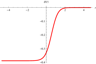
Refer to caption — Figure 1: $\phi(r)$ solution in pure $F(4)$ gauged supergravity.

We now look at the asymptotic behavior of the solution near the critical points. At the UV point, we take $r\rightarrow\infty$ and $A(r)\rightarrow\frac{r}{L_{\textrm{UV}}}$ with $L_{\textrm{UV}}=\frac{1}{2m}$ . The linearized equations of motion give

\phi\sim c_{1}e^{-\frac{3r}{L_{\textrm{UV}}}}+c_{2}e^{-\frac{2r}{L_{\textrm{UV}}}}\,.

(58)

In this case, we find again that the dual operator should be given by a mass term of the scalars in hypermultiplets.
The solution with $c_{1}=0$ and $c_{2}=0$ corresponds to non-normalizable and normalizable modes, respectively. The flow with $c_{1}=0$ is driven by turning on a mass term for hypermultiplet scalars while the flow with $c_{2}=0$ is driven by a vev of this operator. To decide between these two possibilities, we generally need to compute the “superpotential” in the Hamilton-Jacobi formalism for holographic RG flows [33], [34].
However, in this case, there is a simple argument in deciding between a vev deformation and a true deformation by turning on a dual operator as discussed in [17]. The scalar field is negative ( $\phi<0$ ) along the flow. There cannot be any vev deformations since the physical vacuum expectation value, $\langle\mathcal{O}_{\phi}\rangle$ , of a positive definite operator must be positive. Therefore, the scalar $\sigma$ corresponds to turning on a relevant operator of dimension $\Delta=3$ in the dual UV CFT. This is described by the non-normalizable mode $e^{-\frac{2r}{L_{\textrm{UV}}}}$ in (58).
The situation is very similar to the RG flow in minimal gauged supergravity in seven dimensions studied in [28]. The similarity can be made even more explicit by finding the behavior of $\phi(r)$ near the UV point using the “true” superpotential. This gives $\phi(r)\sim e^{-\frac{3r}{L_{\textrm{UV}}}}$ which precisely corresponds to the vev of a dimension $3$ operator.
At the IR point, we find

\phi\sim e^{\frac{\sqrt{65}+5}{2}\frac{r}{L_{\textrm{IR}}}}

(59)

with $L_{\textrm{IR}}=\frac{\sqrt{5}}{2m(3^{\frac{3}{4}})}$ . We see that the corresponding operator is irrelevant and has dimension $\Delta=\frac{\sqrt{65}+5}{2}>5$ . As pointed out in [17], the dual operator acquires an anomalous dimension in the IR. The ratio of the central charges in this case is given by

\frac{c_{\textrm{UV}}}{c_{\textrm{IR}}}=\frac{27}{25}\,.

(60)

5 Conclusions

In this paper, we have studied the scalar potential of $F(4)$ gauged supergravity coupled to three vector multiplets and the corresponding critical points. We have found new critical points apart from the known trivial one with maximal supersymmetry. One of these critical points is supersymmetric with $SO(3)$ symmetry and can be considered as a gravity dual to a new supersymmetric SCFT₅. This should be an IR fixed point of the $N=2$ CFT₅ with symmetry $F(4)\times SO(3)$ . We have also given an analytic solution describing the RG flow between these two critical points. This flow involves two active scalars corresponding to relevant operators of dimension $3$ in the dual field theory. The two scalars transform under $SU(2)_{R}\times SO(3)$ as $(\mathbf{1},\mathbf{1})$ and a combination of $(\mathbf{3},\mathbf{3})$ representations. We have identified these operators with hyper-scalar mass terms. We have shown that the flow is driven by a vacuum expectation value of these operators. Furthermore, we have shown that the non-supersymmetric critical point of the pure $F(4)$ gauged supergravity is unstable in the matter coupled theory.
It is interesting to study the matter coupled $F(4)$ gauged supergravity with other global symmetry group $E_{N_{f}+1}$ in more details. This could give some insights to the dynamics of the D4-brane worldvolume theory in the presence of D8-branes. Furthermore, it would be useful to uplift the flow solution to ten dimensions in the context of massive type IIA theory in which the $F(4)$ gauged supergravity can be embedded [35]. The solution should also be uplifted to type II theory by the truncation given in [36]. With an analytic solution given here, the uplifted solution would be useful in doing a brane probe computation which could give some insight to D-brane dynamics and the corresponding gauge theory.
It is remarkable that we have found a supersymmetric $AdS_{6}$ critical points although a recent result in [37] has pointed out the scarcity of supersymmetric $AdS_{6}$ solutions from massive type IIA supergravity. This makes the embedding of the new supersymmetric $AdS_{6}$ solution discovered here in massive type IIA (if possible) highly non-trivial. Along the line of finding supersymmetric $AdS_{6}$ solutions, we should study the matter coupled $F(4)$ gauged supergravity in more details with possibly different gauge groups to see whether there are any possibilities of $AdS_{6}$ critical points. Moreover, there is another possibility to obtain supersymmetric $AdS_{6}$ by using Hopf T-duality, see for example a discussion in [38], in type IIB theory [39].

Acknowledgments.

I gratefully thank Henning Samtleben for helpful correspondences and valuable comments. I would also like to thank Eoin O. Colgain for pointing out reference [17] and a number of useful discussions. Invaluable suggestions from Carlos Nunez are gratefully acknowledged. This work is partially supported by Thailand Center of Excellence in Physics through the ThEP/CU/2-RE3/11 project and Chulalongkorn University through Ratchadapisek Sompote Endowment Fund.

References

[1] J. M. Maldacena, “The large $N$ limit of superconformal field theories and supergravity”, Adv. Theor. Math. Phys. 2 (1998) 231-252, arXiv: hep-th/9711200.
[2] D.Z. Freedman, S. Gubser, N. Warner and K. Pilch, “Renormalization Group Flows from Holography-Supersymmetry and a c-Theorem”, Adv. Theor. Math. Phys. 3 (1999), arXiv: hep-th/9904017.
[3] Alexei Khavaev and Nicholas P. Warner, “A Class of $N=1$ Supersymmetric RG Flows from Five-dimensional $N=8$ Supergravity”, Phys. Lett. 495 (2000) 215-222, arXiv: hep-th/0009159.
[4] L.Girardello, M.Petrini, M.Porrati and A. Zaffaroni, “Novel Local CFT and exact results on perturbations of $N=4$ super Yang-Mills from AdS dynamics”, JHEP 9812 (1998) 022.
[5] P. Kraus, “Lectures on black holes and the AdS₃/CFT₂ correspondence”, Lect. Notes Phys 755 (2008) 193-247, arXiv: hep-th/0609074.
[6] O. Aharony, O. Bergman, D. L. Jafferis and J. Maldacena, “N=6 superconformal Chern-Simons-matter theories, M2-branes and their gravity duals”, JHEP 10 (2008) 091, arXiv: 0806.1218.
[7] M. Nishimura, “Conformal supergravity from the AdS/CFT correspondence”, Nucl. Phys. B588 (2000) 471-482, arXiv: hep-th/0004179.
[8] A. J. Nurmagambetov and I. Y. Park, “On the M5 and AdS₇/CFT₆ correspondence”, Phys. Lett. B524 (2002) 185-191, arXiv: hep-th/0110192.
[9] S. Nojiri, S. D. Odintsov and S. Ogushi, “Holographic renormalization group and conformal anomaly for AdS₉/CFT₈ correspondence”, Phys. Lett. B500 (2001) 199-208, arXiv: hep-th/0011182.
[10] M. Berg and H. Samtleben, “An exact holographic RG Flow between 2d Conformal Field Theories”, JHEP 05 (2002) 006, arXiv: hep-th/0112154.
[11] Edi Gava, Parinya Karndumri and K. S. Narain, “AdS₃ Vacua and RG Flows in Three Dimensional Gauged Supergravities”, JHEP 04 (2010) 117, arXiv: 1002.3760.
[12] Auttakit Chatrabhuti and Parinya Karndumri, “Vacua and RG flows in $N=9$ three dimensional gauged supergravity”, JHEP 10 (2010) 098, arXiv: 1007.5438.
[13] N. Bobev, N. Halmagyi, K. Pilch and N. P. Warner, “Holographic $N=1$ supersymmetric RG flows on M2 branes”, JHEP 09 (2009) 043, arXiv: 0901.2736.
[14] C. Ahn and K. Woo, “Holographic $N=1$ supersymmetric membrane flows”, Class. Quant. Grav. 27 (2010) 205011, arXiv: 1004.0619.
[15] S. Ferrara, A. Kehagias, H. Partouche, A. Zaffaroni, “AdS₆ interpretation of 5d superconformal field theories”, Phys. Lett. B431 (1998) 57-62, arXiv: hep-th/9804006.
[16] O. Bergman and D. Rodriguez-Gomez, “5d quivers and their AdS(6) duals”, arXiv: 1206.3503.
[17] U. Gursoy, C. Nunez and M. Schvellinger, “RG flows from Spin(7), CY 4-fold and HK manifolds to AdS, Penrose limits and pp waves”, JHEP 06 (2002) 015, arXiv: hep-th/0203124.
[18] L. J. Romans, “The $F(4)$ gauged supergravity in six-dimensions”, Nucl. Phys B269 (1986) 691.
[19] C. Nunez, I. Y. Park, M. Schvellinger and T. A. Tran, “Supergravity duals of gauge theories from F(4) gauged supergravity in six dimensions”, JHEP 04 (2001) 025, arXiv: hep-th/0103080.
[20] R. D’ Auria, S. Ferrara and S. Vaula, “Matter coupled $F(4)$ supergravity and the AdS₆/CFT₅ correspondence”, JHEP 10 (2000) 013, arXiv: hep-th/0006107.
[21] L. Andrianopoli, R. D’ Auria and S. Vaula, “Matter coupled $F(4)$ gauged supergravity Lagrangian”, JHEP 05 (2001) 065, arXiv: hep-th/0104155.
[22] N. Seiberg, “Five dimensional SUSY field theories, non-trivial fixed points and string dynamics”, Phys. Lett. B388 (1996) 753-760, arXiv: hep-th/9608111.
[23] K. Intriligator, D. R. Morrison and N. Seiberg, “Five dimensional supersymmetric gauge theories adn degenerations of Calabi-Yau spaces”, Nucl. Phys. B497 (1997) 56, arXiv: hep-th/9702198.
[24] A. Brandhuber and Y. Oz, “The D4-D8 brane system and five dimensional fixed points”, Phys. Lett. B460 (1999) 307-312, arXiv: hep-th/9905148.
[25] D. R. Morrison and N. Seiberg, “Extremal transitions and five-dimensional supersymmetric field theories”, Nucl. Phys. B483 (1997) 229, arXiv: hep-th/9609070.
[26] E. Bergshoeff, H. Samtleben and E. Sezgin, “The gaugings of maximal D=6 supergravity”, JHEP 03 (2008) 068, arXiv: 0712.4277.
[27] N. P. Warner, “Some New Extrema of the Scalar Potential of Gauged $N=8$ Supergravity”, Phys. Lett. B128 (1983) 169.
[28] V. L. Campos, G. Ferretti, H. Larsson, D. Martelli and B. E. W. Nilsson, “A study of holographic renormalization group flows in $d=6$ and $d=3$ ”, JHEP 06 (2000) 023, arXiv: hep-th/0003151.
[29] J. Babington, D. E. Crooks and N. Evans, “A non-supersymmetric deformation of the AdS/CFT correspondence”, JHEP 02 (2003) 024, arXiv: hep-th/0207076.
[30] J. Distler, F. Zamora, “Non-supersymmetric conformal field theories from stable Anti-de Sitter spaces”, Adv. Theor. Math. Phys. 2 (1999) 1405-1439, arXiv: hep-th/9810206.
[31] E. D’ Hoker and D. Z. Freedman, “Supersymmetric Gauge Theories and the AdS/CFT Correspondence”, TASI 2001 Lecture Notes, arXiv: hep-th/0201253.
[32] K. Skenderis and P. K. Townsend, “Gravitational stability and renormalization-group flow”, Phys. Lett. B468 (1999) 46-51, arXiv: hep-th/9909070.
[33] J. de Boer, E. Verlinde and H. Verlinde, “On the holographic renormalization group”, Nucl. Phys. B550 (1999) 169-182, arXiv: hep-th/9902012.
[34] E. Verlinde and H. Verlinde, “RG-flow, gravity and the cosmological constant”, JHEP 05 (2000) 034, arXiv: hep-th/9912018.
[35] M. Cvetic, H. Lu and C. N. Pope, “Gauged six-dimensional supergravity from massive type IIA”, Phys. Rev. Lett. 83 (1999) 5226-5229, arXiv: hep-th/9906221.
[36] G. Itsios, Y. Lozano, E. O. Colgain and K. Sfetsos, “Non-Abelian T-duality and consistent truncations in type-II supergravity”, arXiv: 1205.2274.
[37] A. Passias, “A note on supersymmetric AdS₆ solutions of massive type IIA supergravity”, arXiv: 1209.3267.
[38] M. Cvetic, H. Lu, C. N. Pope, and J. F. Vazquez-Poritz, “AdS in warped spacetimes”, Phys. Rev. D62 (2000) 122003, arXiv: hep-th/0005246.
[39] E. O. Colgain, private communication.