An explicit effect of non-symmetry of random walks on the triangular lattice

Satoshi Ishiwata , Hiroshi Kawabi and Tsubasa Teruya Note: Department of Mathematical Sciences, Faculty of Science, Yamagata University, 1-4-12, Kojirakawa, Yamagata 990-8560, Japan (e-mail: ishiwata@sci.kj.yamagata-u.ac.jp) Note: Partially supported by Grant-in-Aid for Young Scientists (B)(No. 21740034), JSPS Note: Department of Mathematics, Faculty of Science, Okayama University, 3-1-1, Tsushima-Naka, Kita-ku, Okayama 700-8530, Japan (e-mail: kawabi@math.okayama-u.ac.jp) Note: Partially supported by Grant-in-Aid for Young Scientists (B)(No. 23740107), JSPS Note: The Okinawa Kaiho Bank, Ltd., 2-9-12, Kumoji, Naha, Okinawa 900-8686, Japan

August 24, 2026

Abstract

In the present paper, we study an explicit effect of non-symmetry on asymptotics of the $n$ -step transition probability as $n\rightarrow\infty$ for a class of non-symmetric random walks on the triangular lattice. Realizing the triangular lattice into $\mathbb{R}^{2}$ appropriately, we observe that the Euclidean distance in $\mathbb{R}^{2}$ naturally appears in the asymptotics. We characterize this realization from a geometric view point of Kotani-Sunada’s standard realization of crystal lattices. As a corollary of the main theorem, we prove that the transition semigroup generated by the non-symmetric random walk approximates the heat semigroup generated by the usual Brownian motion on $\mathbb{R}^{2}$ .

1 Introduction

Let $G=(V,E)$ be a locally finite, connected, oriented graph. Here $V$ is the set of vertices and $E$ is the set of oriented edges. For an oriented edge $e\in E$ , the origin and the terminus of $e$ are denoted by $o(e)$ and $t(e)$ , respectively. The inverse edge of $e$ is denoted by $\overline{e}$ . A random walk on $G$ is given by a non-negative valued function $p$ on $E$ satisfying

\sum_{e\in E_{x}}p(e)=1\quad\mbox{for all $x\in V$},

where $E_{x}=\left\{e\in E|~o(e)=x\right\}$ . Here $p(e)$ is the probability that a particle at $o(e)$ moves to $t(e)$ along the edge $e$ in one unit time. Then the transition probability $p(n,x,y)$ that a particle starting at $x\in V$ reaches $y\in V$ at time $n$ is given by

p(n,x,y)=\sum_{c=(e_{1},e_{2},\ldots,e_{n})}p(e_{1})p(e_{2})\cdots p(e_{n}),

where the sum is taken over all paths $c=(e_{1},e_{2},\ldots,e_{n})$ with $t(e_{i})=o(e_{i+1})$ , $i=1,\ldots,n-1$ and $o(e_{1})=x$ , $t(e_{n})=y$ . If there exists a positive valued function $m_{V}$ on $V$ such that

p(e)m_{V}(o(e))=p({\overline{e}})m_{V}(t(e)),\quad e\in E,

the random walk is said to be ( $m_{V}$ -)symmetric.

A principal theme for random walks is to investigate the properties of $p(n,x,y)$ as $n\to\infty$ . One of the most classical problems is the recurrence-transience problem which is related to the divergence-convergence of $\sum_{n=1}^{\infty}p(n,x,x)$ , and the local central limit theorem gives us a useful criterion for the divergence-convergence of the series. For this reason, this theme has been discussed intensively in various settings by many authors. See Spitzer [10], Lawler and Limic [8] and Woess [15] for an overview of random walks.

In particular, Kotani, Shirai and Sunada investigated long time asymptotics of $p(n,x,y)$ of ( $m_{V}$ -)symmetric random walks on a crystal lattice, a covering graph of a finite graph whose covering transformation group is abelian. In [4], as the precision of the local central limit theorem (cf. [7]), they established the asymptotic expansion

p(n,x,y)m_{V}(y)^{-1}\sim a_{0}n^{-r/2}\exp\big(-\frac{d(x,y)^{2}}{4n}\big)\cdot\Big(1+a_{1}(x,y)n^{-1}+a_{2}(x,y)n^{-2}+\cdots\Big)

(1.1)

as $n\to\infty$ , where $d(x,y)$ is a Euclidean distance appeared through the standard realization of the graph into $\mathbb{R}^{r}$ . In their proof, spectral theoretic arguments due to the periodicity of the graph and the symmetry of the random walk play crucial roles.

Later in [2, 14], Uchiyama and his coauthor also established the formula (1.1) for non-symmetric random walks on periodic graphs (i.e., crystal lattices) in the Euclidean space by a probabilistic approach. Their result implies that the effect of the non-symmetry on the coefficient $a_{1}(x,y)$ highly depends not only on the underlying periodic graph but also on the choice of the $1$ -step transition probability $p$ even if the zero mean condition (see condition (P2) in Section 2) is imposed.

In view of these results, it is a meaningful problem to determine an explicit effect of the non-symmetry on the coefficient $a_{1}(x,y)$ on a specific graph. In the present paper, we give an answer of this problem in the case of the triangular lattice. As we will mention later, there exist non-symmetric random walks on the triangular lattice satisfying the zero mean condition (P2). On the other hand, for example, on the square lattice and the hexagonal lattice, we note that the zero mean condition is equivalent to the symmetry of the random walk since these graphs are maximal abelian coverings (see Kotani and Sunada [6, page 842]). In the proof of the main theorem (Theorem 2.2), we make use of the probabilistic approach as in [2, 14] with the idea of the standard realization by Kotani and Sunada [4, 5].

As a corollary of Theorem 2.2, we establish the functional analytic central limit theorem (Theorem 2.4) that the transition semigroup generated by the non-symmetric random walk on the triangular lattice approximates the heat semigroup generated by the usual Brownian motion on $\mathbb{R}^{2}$ . It says that the effect of the non-symmetry of the random walk does not appear in the appropriate space-time scaling limit.

Throughout the present paper, $O(\cdot)$ stands for the Landau symbol. When the dependence of the $O(\cdot)$ term is significant, we specify as $O_{N}(\cdot)$ , etc.

2 Framework and Results

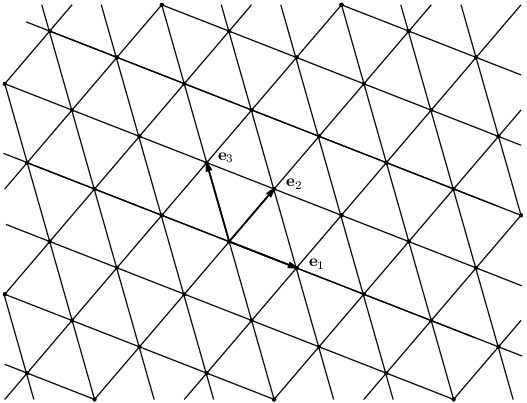
First of all, we prepare some notations and formulate our problem. Let ${\bf e}_{1}$ and ${\bf e}_{2}$ be linearly independent vectors in $\mathbb{R}^{2}$ and we set ${\bf e}_{3}:={\bf e}_{2}-{\bf e}_{1}$ and $K:=\|{\bf e}_{1}\|_{\mathbb{R}^{2}}+\|{\bf e}_{2}\|_{\mathbb{R}^{2}}$ . We define the triangular lattice $G=(V,E)$ by

	$\displaystyle V$	$\displaystyle=\{x=x_{1}{\bf e}_{1}+x_{2}{\bf e}_{2}\|~(x_{1},x_{2})\in{\mathbb{Z}}^{2}\},$
	$\displaystyle E$	$\displaystyle=\left\{(x,y)\in V\times V\|~x-y\in\left\{\pm{\bf e}_{1},\pm{\bf e}_{2},\pm{\bf e}_{3}\right\}\right\}$

(see Figure 1).

Refer to caption — Figure 1: Triangular lattice

We remark that $G$ is isomorphic to the Cayley graph of the abelian group $\mathbb{Z}^{2}$ with a set of generators $S=\{\pm(1,0),\pm(0,1),\pm(-1,1)\}$ identified by $V\simeq\mathbb{Z}^{2}$ and $\mathbf{e}_{1}\simeq(1,0)$ , $\mathbf{e}_{2}\simeq(0,1)$ , $\mathbf{e}_{3}\simeq(-1,1)$ .

Throughout the present paper, we impose the following conditions on the $1$ -step transition probability $p$ :

(P1):

For every $x\in V$ ,

	$\displaystyle p\big((x,x+{\bf e}_{1})\big)$	$\displaystyle=\alpha,\quad p\big((x,x-{\bf e}_{1})\big)=\alpha^{\prime},$
	$\displaystyle p\big((x,x+{\bf e}_{2})\big)$	$\displaystyle=\beta^{\prime},\quad p\big(x,x-{\bf e}_{2})\big)=\beta,$
	$\displaystyle p\big((x,x+{\bf e}_{3})\big)$	$\displaystyle=\gamma,\quad p\big((x,x+{\bf e}_{3})\big)=\gamma^{\prime},$

where $\alpha,\alpha^{\prime},\beta,\beta^{\prime},\gamma,\gamma^{\prime}\geq 0$ and $\alpha+\alpha^{\prime}+\beta+\beta^{\prime}+\gamma+\gamma^{\prime}=1$ .

(P2):

Zero mean condition:

\sum_{e\in E_{0}}p(e)e=0.

(P3):

\Gamma(p):={\widehat{\alpha}}{\widehat{\beta}}+{\widehat{\beta}}{\widehat{\gamma}}+{\widehat{\gamma}}{\widehat{\alpha}}>0,

where ${\widehat{\alpha}}:=\alpha+\alpha^{\prime},{\widehat{\beta}}:=\beta+\beta^{\prime},{\widehat{\gamma}}:=\gamma+\gamma^{\prime}$ .

Remark 2.1

Condition (P2) is equivalent to the following condition:

$\bullet$ There exists a constant $0\leq\kappa\leq\frac{1}{3}$ such that $\alpha-\alpha^{\prime}=\beta-\beta^{\prime}=\gamma-\gamma^{\prime}=\kappa$ .

In the case $\kappa=0$ , condition (P2) implies that $p(e)=p({\overline{e}})$ holds for every $e\in E$ . Namely, our random walk is symmetric with $m_{V}\equiv 1$ . On the other hand, by a simple calculation, we see that there does not exist the function $m_{V}$ satisfying (1) unless $\kappa=0$ . Hence our random walk is non-symmetric in the case $0<\kappa\leq\frac{1}{3}$ . We can regard the constant $\kappa$ as intensity of the non-symmetry.

We set

M_{q}(\theta):=\sum_{e\in E_{0}}p(e)\langle e,\theta\rangle^{q},\quad\theta=(\theta_{1},\theta_{2})\in\mathbb{R}^{2},q\in\mathbb{N},

(2.1)

where $\langle\cdot,\cdot\rangle$ stands for the scalar product on $\mathbb{R}^{2}$ . Note that condition (P2) implies $M_{1}(\theta)\equiv 0$ . By condition (P1), we also have

|M_{q}(\theta)|\leq\big(\sum_{e\in E_{0}}p(e)\|e\|_{\mathbb{R}^{2}}^{q}\big)\|\theta\|_{\mathbb{R}^{2}}^{q}\leq K^{q}\|\theta\|_{\mathbb{R}^{2}}^{q},\quad\theta\in\mathbb{R}^{2},q\in\mathbb{N}.

(2.2)

We define the covariance matrix $Q$ by

\langle Q\theta,\theta\rangle=M_{2}(\theta),\quad\theta\in\mathbb{R}^{2}.

In the case of ${\bf e}_{1}={\widehat{\bf e}}_{1}:=\hskip-2.84526pt\mbox{ }^{t}(1,0)$ and ${\bf e}_{2}={\widehat{\bf e}}_{2}:=\hskip-2.84526pt\mbox{ }^{t}(0,1)$ , the corresponding covariance matrix is easily calculated as

{\widehat{Q}}:=\left(\begin{array}[]{cc}{\widehat{\alpha}}+{\widehat{\gamma}}&-{\widehat{\gamma}}\\ -{\widehat{\gamma}}&{\widehat{\beta}}+{\widehat{\gamma}}\end{array}\right),

and hence we obtain ${\rm det}{\widehat{Q}}=\Gamma(p)$ . For a general pair of two vectors ${\bf e}_{1}$ , ${\bf e}_{2}$ , we can decompose the covariance matrix $Q$ as

Q=T{\widehat{Q}}\hskip-2.84526pt\mbox{ }^{t}T,

(2.3)

where $T=[{\bf e}_{1},{\bf e}_{2}]$ stands for the matrix formed by column vectors ${\bf e}_{1},{\bf e}_{2}$ . It follows from condition (P3) and linear independence of ${\bf e}_{1}$ , ${\bf e}_{2}$ that the covariance matrix $Q$ is positive definite, i.e., $\langle\theta,Q\theta\rangle\geq\lambda\|\theta\|^{2}_{\mathbb{R}^{2}},\theta\in\mathbb{R}^{2}$ for some $\lambda>0$ . By (2.3), we also observe that

\langle Q^{-1}x,y\rangle=\langle{\widehat{Q}}^{-1}(x_{1}{\widehat{\bf e}_{1}}+x_{2}{\widehat{\bf e}_{2}}),y_{1}{\widehat{\bf e}_{1}}+y_{2}{\widehat{\bf e}_{2}}\rangle

(2.4)

holds for all $x=x_{1}{\bf e}_{1}+x_{2}{\bf e}_{2},y=y_{1}{\bf e}_{1}+y_{2}{\bf e}_{2}\in V$ . This means that the left-hand side of (2.4) is independent of the realization of the triangular lattice $G$ .

Now, we are in a position to state our main result. Let

A(G):=\frac{1}{3\Gamma(p)^{1/2}},\quad l:=\left(\frac{\widehat{\beta}+\widehat{\gamma}}{3\Gamma(p)}\right)^{1/2}

(2.5)

and we introduce two vectors by

{\mathbf{h}}_{1}:=\hskip-2.84526pt\mbox{ }^{t}(l,0),\quad{\mathbf{h}}_{2}:=\hskip-2.84526pt\mbox{ }^{t}\Big(\frac{\widehat{\gamma}}{{\widehat{\beta}}+{\widehat{\gamma}}}l,\frac{\Gamma(p)^{1/2}}{\widehat{\beta}+\widehat{\gamma}}l\Big)

(see Figure 2).

Note that $A(G)$ is equal to the area of the parallelogram spanned by $\mathbf{h}_{1}$ and $\mathbf{h}_{2}$ . In the case of ${\bf e}_{1}={\mathbf{h}}_{1}$ and ${\bf e}_{2}={\mathbf{h}}_{2}$ , the corresponding covariance matrix is

Q=\left(\begin{array}[]{cc}1/3&0\\ 0&1/3\end{array}\right).

(2.6)

Realizing the triangular lattice $G$ along these two vectors, we have

Theorem 2.2

(1) Let us consider the case $0\leq\kappa<1/3$ . Then we have

	$\displaystyle 2\pi n\cdot p(n,x,y)$	$\displaystyle=$	$\displaystyle 3A(G)\exp\Big(-\frac{3}{2n}\\|y-x\\|^{2}_{\mathbb{R}^{2}}\Big)$
			$\displaystyle\times\Big(1+\sum_{j=1}^{N}n^{-j/2}P_{j}\Big(\frac{y-x}{\sqrt{n}}\Big)\Big)+O_{N}\big(n^{-\frac{N+1}{2}}\big),\quad N\in\mathbb{N}\cup\{0\},$

as $n\rightarrow\infty$ uniformly for all $x,y\in V$ , where $P_{j}=P_{j}(y)$ , $j\in\mathbb{N}$ is a polynomial of degree at most $3j$ in the variables $y_{1},y_{2}$ and an odd or even function depending on whether $j$ is odd or even. Furthermore, let us denote the leading term of $\sum_{j=1}^{N}n^{-j/2}P_{j}\big(\frac{y-x}{\sqrt{n}}\big),N\geq 2$ by $a_{1}(y-x;\kappa)n^{-1}$ , that is,

\lim_{n\to\infty}n\Big(\sum_{j=1}^{N}n^{-j/2}P_{j}\Big(\frac{y-x}{\sqrt{n}}\Big)-a_{1}(y-x;\kappa)n^{-1}\Big)=0,\quad x,y\in V.

Then the coefficient $a_{1}(y;\kappa)$ is explicitly obtained by

a_{1}(y;k)=a_{1}^{(0)}+\kappa a_{1}^{(1)}(y)+{\kappa}^{2}a_{1}^{(2)},

where

	$\displaystyle a_{1}^{(0)}$	$\displaystyle=-1+\frac{1}{8\Gamma(p)^{2}}\left\{\widehat{\alpha}(\widehat{\beta}+\widehat{\gamma})^{2}+\widehat{\beta}(\widehat{\gamma}+\widehat{\alpha})^{2}+\widehat{\gamma}(\widehat{\alpha}+\widehat{\beta})^{2}\right\},$
	$\displaystyle a_{1}^{(1)}(y)$	$\displaystyle=\frac{1}{\Gamma(p)^{2}}\left\{(\widehat{\alpha}\widehat{\beta}-2\widehat{\beta}\widehat{\gamma}+\widehat{\gamma}\widehat{\alpha})y_{1}+(-\widehat{\alpha}\widehat{\beta}-\widehat{\beta}\widehat{\gamma}+2\widehat{\gamma}\widehat{\alpha})y_{2}\right\},\quad y=y_{1}\mathbf{h}_{1}+y_{2}\mathbf{h}_{2},$
	$\displaystyle a_{1}^{(2)}$	$\displaystyle=\frac{3}{8\Gamma(p)^{2}}\Big(-1+\frac{5\widehat{\alpha}\widehat{\beta}\widehat{\gamma}}{\Gamma(p)}\Big).$

(2) Let us consider the case $\kappa=1/3$ , i.e., $\alpha=\beta=\gamma=1/3$ , $\alpha^{\prime}=\beta^{\prime}=\gamma^{\prime}=0$ . We set

V_{k}:=\big\{x=x_{1}\widetilde{\mathbf{h}}_{1}+x_{2}\widetilde{\mathbf{h}}_{2}\ |\ (x_{1},x_{2})\in\mathbb{Z}^{2}\big\}+k{\mathbf{h}}_{1},\quad k=0,1,2,

where $\widetilde{\mathbf{h}}_{1}=2\mathbf{h}_{1}-\mathbf{h}_{2}$ , $\widetilde{\mathbf{h}}_{2}=\mathbf{h}_{1}+\mathbf{h}_{2}$ , $\mathbf{h}_{1}=\!^{t}(\sqrt{2/3},0)$ , $\mathbf{h}_{2}=\!^{t}(1/\sqrt{6},1/\sqrt{2})$ (see Figure 3). For $k,l=0,1,2$ , we take $x\in V_{k}$ and $y\in V_{l}$ . Then we have

	$\displaystyle 2\pi n\cdot p(n,x,y)$	$\displaystyle=$	$\displaystyle 9A(G)\exp\Big(-\frac{3}{2n}\\|y-x\\|^{2}_{\mathbb{R}^{2}}\Big)$
			$\displaystyle\times\Big(1+\sum_{j=1}^{N}n^{-j/2}P_{j}\Big(\frac{y-x}{\sqrt{n}}\Big)\Big)+O_{N}\big(n^{-\frac{N+1}{2}}\big),\quad N\in\mathbb{N}\cup\{0\}$

as $n=3m+(l-k)\rightarrow\infty$ uniformly for all $x$ and $y$ . In this case, $A(G)=1/{\sqrt{3}}$ and the coefficient of the leading term is

a_{1}(y-x;1/3)=-\frac{2}{3}.

We characterize the pair $\mathbf{h}_{1}$ , $\mathbf{h}_{2}$ through a variational problem on the crystal lattices based on the idea of Kotani and Sunada [4, 5].

We set ${\bf e}_{1}:=\!^{t}(u,0),{\bf e}_{2}:=\!^{t}(v_{1},v_{2})$ . Without loss of generality, we may assume $u,v_{2}>0$ . Then the energy of the (quotient graph of the) triangular lattice $G$ is given by

	$\displaystyle{\cal E}(G)$	$\displaystyle:=$	$\displaystyle\frac{1}{2}\sum_{e\in E_{0}}p(e)\\|t(e)-o(e)\\|^{2}_{\mathbb{R}^{2}}$
		$\displaystyle=$	$\displaystyle\frac{1}{2}\Big[{\widehat{\alpha}}u^{2}+{\widehat{\beta}}(v_{1}^{2}+v_{2}^{2})+{\widehat{\gamma}}\big\{(v_{1}-u)^{2}+v_{2}^{2}\big\}\Big].$

Minimizing ${\cal E}(G)$ with respect to $(u,v_{1},v_{2})$ under the condition ${\rm det}(\langle{\bf e}_{i},{\bf e}_{j}\rangle)_{i,j=1}^{2}=A(G)$ , we obtain

u=l,\quad v_{1}=\frac{\widehat{\beta}}{\widehat{\beta}+\widehat{\gamma}}l,\quad v_{2}=\frac{\Gamma(p)^{1/2}}{\widehat{\beta}+\widehat{\gamma}}l.

Hence we have derived $\mathbf{e}_{1}=\mathbf{h}_{1}$ , $\mathbf{e}_{2}=\mathbf{h}_{2}$ .

Remark 2.3

In the case $\alpha=\alpha^{\prime}=\beta=\beta^{\prime}=\gamma=\gamma^{\prime}=1/6,$ the random walk is said to be simple. In this case, we have

A(G)=\frac{1}{\sqrt{3}},\quad l=\sqrt{\frac{2}{3}},\quad\mathbf{h}_{1}=\!^{t}\left(\sqrt{\frac{2}{3}},0\right),\quad\mathbf{h}_{2}=\!^{t}\left(\frac{1}{\sqrt{6}},\frac{1}{\sqrt{2}}\right).

We note the volume of the Albanese torus is equal to $1/\sqrt{3}$ (see [4, page 640], [7, Section 10] ). The standard realization of the triangular lattice is the equilateral triangular lattice in $\mathbb{R}^{2}$ each of whose edge has length $\sqrt{2/3}$ . The quantity $A(G)$ introduced in (2.5) can be regarded as a generalization of the notion of the volume of the Albanese torus to some non-symmetric cases. Henceforth, we call the realization of the triangular lattice $G$ along $\mathbf{h}_{1}$ and $\mathbf{h}_{2}$ the standard realization even if the random walk is non-symmetric.

Next, let us consider the discrete heat equation on the triangular lattice $G=(V,E)$ with initial condition $u_{0}:V\to\mathbb{R}$ :

\left\{\begin{array}[]{rl}\left(\partial_{1}+\Delta_{d}\right)u(n,x)&=0,\qquad(n,x)\in{\mathbb{Z}}_{+}\times V,\\ u(0,x)&=u_{0}(x),\qquad x\in V.\end{array}\right.

(2.7)

Here $\partial_{1}u(n,x):=u(n+1,x)-u(n,x)$ and the discrete Laplacian $\Delta_{d}$ is defined by

\Delta_{d}u(n,x):=\sum_{e\in E_{x}}p(e)\Big(u(n,o(e))-u(n,t(e))\Big).

The operator $L:=I-\Delta_{d}$ is called the transition operator associated with the random walk on $G$ . It is easy to see that the solution of (2.7) is given by

u(n,x)=L^{n}u_{0}(x).

We note that the solution is rewritten by

u(n,x)=\sum_{y\in V}p(n,x,y)u_{0}(y).

For $t>0$ , let $H_{t}$ be the heat operator defined by

H_{t}f(x)=\frac{1}{2\pi t}\int_{\mathbb{R}^{2}}\exp\Big(-\frac{\|x-z\|_{\mathbb{R}^{2}}^{2}}{2t}\Big)f(z)dz,\quad f\in C_{\infty}(\mathbb{R}^{2}),

where $C_{\infty}(\mathbb{R}^{2})$ is the set of continuous functions on $\mathbb{R}^{2}$ vanishing at infinity. Note that $\{H_{t}\}_{t\geq 0}$ is a semigroup whose infinitesimal generator is

\frac{1}{2}\Delta:=\frac{1}{2}\left(\frac{\partial^{2}}{\partial x_{1}^{2}}+\frac{\partial^{2}}{\partial x_{2}^{2}}\right).

Now, we take the standard realization of the triangular lattice $G$ as before. Applying Theorem 2.2, we obtain the following.

Theorem 2.4

Let $t>0$ and $\{\delta_{n}\}_{n=1}^{\infty}$ be a sequence of positive real numbers satisfying $\lim_{n\to\infty}n\delta_{n}^{2}=3t$ . Then for every continuous function $f$ on $\mathbb{R}^{2}$ with compact support and for a sequence $\{x_{n}\}_{n=1}^{\infty}$ in $V$ with $\lim_{n\rightarrow\infty}\delta_{n}x_{n}=x\in\mathbb{R}^{2}$ , we have

\lim_{n\rightarrow\infty}L^{n}(f\circ\delta_{n})(x_{n})=H_{t}f(x).

This theorem is also an immediate consequence of the following result via approximation theory due to Trotter [13] (see also Kotani [3]).

Theorem 2.5

(1)

\lim_{\delta\rightarrow 0}\left\|\frac{3}{\delta^{2}}\Delta_{d}(f\circ\delta)+\frac{1}{2}(\Delta f)\circ\delta\right\|_{\infty}=0,\quad f\in C^{\infty}_{0}(\mathbb{R}^{2})

(2)

Let $\{\delta_{n}\}_{n=1}^{\infty}$ be a sequence as in Theorem 2.4.

\lim_{n\rightarrow\infty}\|L^{n}(f\circ\delta_{n})-(H_{t}f)\circ\delta_{n}\|_{\infty}=0,\quad f\in C_{\infty}(\mathbb{R}^{2}).

3 Preliminaries

In this section, we give some basic facts for the proof of Theorem 2.2. In what follows, we denote ${\bf h}_{3}:={\bf h}_{2}-{\bf h}_{1}$ , $x_{3}:=x_{2}-x_{1}$ and $(\frac{\partial}{\partial x_{3}}):=(\frac{\partial}{\partial x_{2}})-(\frac{\partial}{\partial x_{1}})$ for convenience.

We begin with the explicit form of $M_{q}(\theta),q\in\mathbb{N}$ defined in (2.1).

Lemma 3.1

We have

M_{q}(\theta)=\begin{cases}{\kappa}\big(\langle{\bf e}_{1},\theta\rangle^{q}-\langle{\bf e}_{2},\theta\rangle^{q}+\langle{\bf e}_{3},\theta\rangle^{q}\big)&\text{ (if $q$ is odd) },\\ {\widehat{\alpha}}\langle{\bf e}_{1},\theta\rangle^{q}+{\widehat{\beta}}\langle{\bf e}_{2},\theta\rangle^{q}+{\widehat{\gamma}}\langle{\bf e}_{3},\theta\rangle^{q}&\text{ (if $q$ is even)}.\end{cases}

In particular, $M_{q}(\theta)\equiv 0$ for every odd number $q$ in the case where the random walk is symmetric.

Noting (2.4) and (2.6), we easily see $\langle Q^{-1}{\bf e}_{i},{\bf e}_{j}\rangle=3\langle{\bf h}_{i},{\bf h}_{j}\rangle,i=1,2,3$ . A direct calculation of the inner product $\langle{\bf h}_{i},{\bf h}_{j}\rangle,i,j=1,2,3$ yields the following lemma:

Lemma 3.2

For any pair of linearly independent vectors ${\bf e}_{1},{\bf e}_{2}\in\mathbb{R}^{2}$ , we have

	$\displaystyle\langle Q^{-1}{\bf e}_{1},{\bf e}_{1}\rangle$	$\displaystyle=$	$\displaystyle\frac{\widehat{\beta}+\widehat{\gamma}}{\Gamma(p)},\quad\langle Q^{-1}{\bf e}_{2},{\bf e}_{2}\rangle=\frac{\widehat{\gamma}+\widehat{\alpha}}{\Gamma(p)},\quad\langle Q^{-1}{\bf e}_{3},{\bf e}_{3}\rangle=\frac{\widehat{\alpha}+\widehat{\beta}}{\Gamma(p)},$
	$\displaystyle\langle Q^{-1}{\bf e}_{1},{\bf e}_{2}\rangle$	$\displaystyle=$	$\displaystyle\frac{\widehat{\gamma}}{\Gamma(p)},\qquad\langle Q^{-1}{\bf e}_{2},{\bf e}_{3}\rangle=\frac{\widehat{\alpha}}{\Gamma(p)},\qquad\langle Q^{-1}{\bf e}_{3},{\bf e}_{1}\rangle=\frac{-\widehat{\beta}}{\Gamma(p)}.$

Next, we recall an elementary fact about the Fourier transform

\int_{\mathbb{R}^{2}}e^{-\frac{1}{2}\langle Q\theta,\theta\rangle}e^{-{\sqrt{-1}}\langle x,\theta\rangle}d\theta=2\pi({\rm det}Q)^{-1/2}e^{-\frac{1}{2}\langle Q^{-1}x,x\rangle},\quad x\in\mathbb{R}^{2}.

(3.1)

Differentiating both sides of (3.1) with respect to $x_{i},~i=1,2,3$ , we have

	$\displaystyle\int_{\mathbb{R}^{2}}\langle{\bf e}_{i},\theta\rangle e^{-\frac{1}{2}\langle Q\theta,\theta\rangle}e^{-{\sqrt{-1}}\langle x,\theta\rangle}d\theta$
		$\displaystyle=$	$\displaystyle 2\pi{\sqrt{-1}}\cdot({\rm det}Q)^{-1/2}\big(-\langle Q^{-1}{\bf e}_{i},x\rangle\big)e^{-\frac{1}{2}\langle Q^{-1}x,x\rangle},\quad x\in\mathbb{R}^{2},i=1,2,3.$

Repeating this argument several times, we obtain the following proposition:

Proposition 3.3

Let us set

F(i_{1},\ldots,i_{N})(x):=\int_{\mathbb{R}^{2}}\big(\prod_{k=1}^{N}\langle{\bf e}_{i_{k}},\theta\rangle\big)e^{-\frac{1}{2}\langle Q\theta,\theta\rangle}e^{-{\sqrt{-1}}\langle x,\theta\rangle}d\theta,\quad N\in\mathbb{N},~i_{1},\ldots,i_{N}=1,2,3.

Then we have

F(i_{1},\ldots,i_{N})(x)=2\pi({\sqrt{-1}})^{N}({\rm det}Q)^{-1/2}e^{-\frac{1}{2}\langle Q^{-1}x,x\rangle}G(i_{1},\ldots,i_{N})(x),

where $\{G(i_{1},\ldots,i_{k})(x):x\in\mathbb{R}^{2},k=1,\ldots,N\}$ is determined as the solution of the recursive system of the following equations starting from $k=1$ to $k=N$ :

\left\{\begin{array}[]{ll}G(i_{1},\ldots,i_{k})(x)=-\langle Q^{-1}{\bf e}_{i_{k}},x\rangle G(i_{1},\ldots,i_{k-1})(x)+{\displaystyle{\frac{\partial}{\partial x_{i_{k}}}G(i_{1},\ldots,i_{k-1})(x)}},\\ \\ G(i_{1})(x)=-\langle Q^{-1}{\bf e}_{i_{1}},x\rangle.\end{array}\right.

(3.2)

Remark 3.4

$G(i_{1},\ldots,i_{N})(x)$ is decomposed by

G(i_{1},\ldots,i_{N})(x)=\begin{cases}\displaystyle{\sum_{l=0}^{\frac{N-1}{2}}G(i_{1},\ldots,i_{N})_{(2l+1)}(x)}&\text{ (if $N$ is odd)},\\ \displaystyle{\sum_{l=0}^{\frac{N}{2}}G(i_{1},\ldots,i_{N})_{(2l)}(x)}&\text{ (if $N$ is even) },\end{cases}

where $G(i_{1},\ldots,i_{N})_{(k)}(x)$ , $k=0,1,\ldots,N$ is a homogeneous polynomial of degree $k$ in the variables $\langle Q^{-1}{\bf e}_{1},x\rangle$ , $\langle Q^{-1}{\bf e}_{2},x\rangle$ and $\langle Q^{-1}{\bf e}_{3},x\rangle$ . In particular,

$\displaystyle G(i_{1},i_{2})(x)$	$\displaystyle=$	$\displaystyle\langle Q^{-1}{\bf e}_{i_{1}},x\rangle\langle Q^{-1}{\bf e}_{i_{2}},x\rangle-\langle Q^{-1}{\bf e}_{i_{1}},{\bf e}_{i_{2}}\rangle,\qquad i_{1},i_{2}=1,2,3,$
$\displaystyle G(i_{1},i_{2},i_{3})(x)$	$\displaystyle=$	$\displaystyle-\langle Q^{-1}{\bf e}_{i_{1}},x\rangle\langle Q^{-1}{\bf e}_{i_{2}},x\rangle\langle Q^{-1}{\bf e}_{i_{3}},x\rangle$
		$\displaystyle+\langle Q^{-1}{\bf e}_{i_{1}},{\bf e}_{i_{2}}\rangle\langle Q^{-1}{\bf e}_{i_{3}},x\rangle+\langle Q^{-1}{\bf e}_{i_{2}},{\bf e}_{i_{3}}\rangle\langle Q^{-1}{\bf e}_{i_{1}},x\rangle$
		$\displaystyle+\langle Q^{-1}{\bf e}_{i_{3}},{\bf e}_{i_{1}}\rangle\langle Q^{-1}{\bf e}_{i_{2}},x\rangle,\qquad i_{1},i_{2},i_{3}=1,2,3.$

We define the characteristic function of the $1$ -step transition probability $p$ by

\varphi(\theta):=\sum_{e\in E_{0}}p(e)\exp\{{\sqrt{-1}}\langle e,\theta\rangle\},\quad\theta=(\theta_{1},\theta_{2})\in\mathbb{R}^{2}.

We denote $\varphi$ especially by $\phi$ in the case of ${\bf e}_{1}={\widehat{\bf e}}_{1}$ and ${\bf e}_{2}={\widehat{\bf e}}_{2}$ . Noting that the characteristic function of the $n$ -step transition probability of the random walk starting at the origin is equal to $\varphi^{n}$ , we have the following integral expression of $p(n,x,y)$ .

Lemma 3.5

p(n,x,y)=\frac{|{\rm det}T|}{(2\pi)^{2}}\int_{(\hskip-2.84526pt\mbox{ }^{t}T)^{-1}(D)}\varphi(\theta)^{n}\exp\{-\sqrt{-1}\langle y-x,\theta\rangle\}d\theta,\quad x,y\in V,~n\in\mathbb{N},

where $D:=[-\pi,\pi]^{2}$ .

Proof. Since $p(n,x,y)=p(n,0,y-x)$ , we may suppose $x=0$ . We also note that $p(n,0,y)$ , $y=y_{1}{{\bf e}}_{1}+y_{2}{{\bf e}}_{2}$ is independent of the pair of linearly independent two vectors ${\bf e}_{1},{\bf e}_{2}$ . In the case ${\bf e}_{1}={\widehat{\bf e}}_{1}$ , ${\bf e}_{2}={\widehat{\bf e}}_{2}$ , the following identity is well-known:

p(n,0,y)=\frac{1}{(2\pi)^{2}}\int_{D}\phi(\theta)^{n}\exp\big\{-\sqrt{-1}\sum_{i=1}^{2}y_{i}\theta_{i}\big\}d\theta,\quad y=y_{1}{\widehat{\bf e}}_{1}+y_{2}{\widehat{\bf e}}_{2},~n\in\mathbb{N}.

(3.3)

See Lawler and Limic [8, Section 2.2.2] for details.

For a general pair of independent two vectors ${{\bf e}}_{1},{{\bf e}}_{2}$ , we observe

\varphi(\theta)=\phi(\hskip-2.84526pt\mbox{ }^{t}T\theta),\quad\theta\in\mathbb{R}^{2}.

(3.4)

Then it follows from (3.3) and (3.4) that

$\displaystyle\frac{1}{(2\pi)^{2}}\int_{D}\phi(\theta)^{n}\exp\big\{-\sqrt{-1}\sum_{i=1}^{2}y_{i}\theta_{i}\big\}d\theta$
	$\displaystyle=$	$\displaystyle\frac{1}{(2\pi)^{2}}\int_{D}\varphi\big((\hskip-2.84526pt\mbox{ }^{t}T)^{-1}\theta\big)^{n}\exp\big\{-\sqrt{-1}\big\langle\sum_{i=1}^{2}y_{i}T{\widehat{\bf e}}_{i},(\hskip-2.84526pt\mbox{ }^{t}T)^{-1}\theta\big\rangle\big\}d\theta$
	$\displaystyle=$	$\displaystyle\frac{1}{(2\pi)^{2}}\int_{D}\varphi\big((\hskip-2.84526pt\mbox{ }^{t}T)^{-1}\theta\big)^{n}\exp\big\{-\sqrt{-1}\langle y,(\hskip-2.84526pt\mbox{ }^{t}T)^{-1}\theta\rangle\big\}d\theta$
	$\displaystyle=$	$\displaystyle\frac{\|{\rm det}T\|}{(2\pi)^{2}}\int_{(\hskip-2.84526pt\mbox{ }^{t}T)^{-1}(D)}\varphi(\theta^{\prime})^{n}\exp\{-\sqrt{-1}\langle y,\theta^{\prime}\rangle\}d\theta^{\prime},\quad y=y_{1}{{\bf e}}_{1}+y_{2}{{\bf e}}_{2},~n\in\mathbb{N},$

where we performed the change of variables $\theta=\hskip-2.84526pt\mbox{ }^{t}T\theta^{\prime}$ for the final line. This completes the proof.

Lemma 3.6

(1) In the case $0\leq\kappa<1/3$ , the characteristic function $\varphi(\theta)$ defined on $(\hskip-2.84526pt\mbox{ }^{t}T)^{-1}(D)$ has the following property: $|\varphi(\theta)|=1$ holds only when $\theta=0$ .
(2) In the case $\kappa=1/3$ , the characteristic function $\varphi(\theta)$ does not satisfy the above property.

Proof. First, we prove (1). By (3.4), it is sufficient to show that $|\phi(\theta)|=1,\theta\in D$ implies $\theta=0$ . We calculate the characteristic function $\phi(\theta)$ as

$\displaystyle\phi(\theta)$	$\displaystyle=$	$\displaystyle\big({\widehat{\alpha}}\cos(\theta_{1})+\sqrt{-1}k\sin(\theta_{1})\big)+\big({\widehat{\beta}}\cos(-\theta_{2})+\sqrt{-1}k\sin(-\theta_{2})\big)$	(3.5)
		$\displaystyle+\big({\widehat{\gamma}}\cos(\theta_{2}-\theta_{1})+\sqrt{-1}k\sin(\theta_{2}-\theta_{1})\big)$
	$\displaystyle=:$	$\displaystyle\phi_{1}(\theta)+\phi_{2}(\theta)+\phi_{3}(\theta),\quad\theta=(\theta_{1},\theta_{2})\in D.$

Note that the assumption $0\leq\kappa<\frac{1}{3}$ implies $\min\{{\widehat{\alpha}},{\widehat{\beta}},{\widehat{\gamma}}\}>\kappa\geq 0$ . Then we have

|\phi_{1}(\theta)|\leq{\widehat{\alpha}},\quad|\phi_{2}(\theta)|\leq{\widehat{\beta}},\quad|\phi_{3}(\theta)|\leq{\widehat{\gamma}},\quad\theta=(\theta_{1},\theta_{2})\in D.

(3.6)

We also observe that and $|\phi_{1}(\theta)|={\widehat{\alpha}},|\phi_{2}(\theta)|={\widehat{\beta}}$ and $|\phi_{3}(\theta)|={\widehat{\gamma}}$ imply $\phi_{1}(\theta)=\pm{\widehat{\alpha}}$ , $\phi_{2}(\theta)=\pm{\widehat{\beta}}$ and $\phi_{3}(\theta)=\pm{\widehat{\gamma}}$ , respectively.

Now, we suppose $|\phi(\theta)|=1$ on $D$ . By combining (3.5) and (3.6) with ${\widehat{\alpha}}+{\widehat{\beta}}+{\widehat{\gamma}}=1$ , we deduce

(\phi_{1}(\theta),\phi_{2}(\theta),\phi_{3}(\theta))=({\widehat{\alpha}},{\widehat{\beta}},{\widehat{\gamma}}),(-{\widehat{\alpha}},-{\widehat{\beta}},-{\widehat{\gamma}}),\quad\theta\in D.

We easily see that the first equation $(\phi_{1}(\theta),\phi_{2}(\theta),\phi_{3}(\theta))=({\widehat{\alpha}},{\widehat{\beta}},{\widehat{\gamma}})$ has the solution $(\theta_{1},\theta_{2})=(0,0)$ . On the other hand, there exists no solution of the second equation $(\phi_{1}(\theta),\phi_{2}(\theta),\phi_{3}(\theta))=(-{\widehat{\alpha}},-{\widehat{\beta}},-{\widehat{\gamma}})$ . Hence we conclude $\theta=0$ , which completes the proof of (1).

The item (2) is obvious by recalling $\alpha=\beta=\gamma=1/3$ and $\alpha^{\prime}=\beta^{\prime}=\gamma^{\prime}=0$ . Actually, $|\phi(\theta)|=1$ on $D$ implies $(\theta_{1},\theta_{2})=(0,0),(\frac{2\pi}{3},-\frac{2\pi}{3})$ , $(-\frac{2\pi}{3},\frac{2\pi}{3})$ .

Remark 3.7

In the case $0\leq\kappa<1/3$ , the random walk is aperiodic, that is, the period of the random walk $d(p):={\rm gcd}\{n\in\mathbb{N}:p(n,0,0)>0\}$ is equal to $1$ . It is derived from (1) of Lemma 3.6. See e.g., Spitzer [10, P8 in Section 7] for the proof. On the other hand, the random walk is periodic with $d(p)=3$ in the case $\kappa=1/3$ .

Before closing this section, we present an asymptotic expansion formula of the characteristic function $\varphi$ which plays a crucial role in the next section. We set

\chi_{q}(\theta):=({\sqrt{-1}})^{-q}\big(\frac{d}{dt}\big)^{q}\Big|_{t=0}\log\varphi(t\theta),\quad\theta\in\mathbb{R}^{2},q\in\mathbb{N}.

(3.7)

(See Bhattacharya and Ranga Rao [1, page 47].) We note that $\chi_{q}(\theta)$ is a polynomial in the variables $M_{2}(\theta),\ldots,M_{q}(\theta)$ . In particular, $\chi_{1}(\theta)\equiv 0,\chi_{2}(\theta)=M_{2}(\theta),\chi_{3}(\theta)=M_{3}(\theta)$ and $\chi_{4}(\theta)=M_{4}(\theta)-3M_{2}(\theta)^{2}$ .

The following proposition is taken from [1, Lemma 7.1 and Theorem 9.11].

Proposition 3.8

Let $n\in\mathbb{N}$ and $N\in\mathbb{N}\cup\{0\}$ . Then there exist positive constants $C_{1}(N),C_{2}(N)$ such that for all $\theta\in\mathbb{R}^{2}$ with

\langle Q\theta,\theta\rangle^{1/2}\leq C_{1}(N)\Big(\sum_{e\in E_{0}}p(e)\langle Q^{-1}e,e\rangle^{N/2}\Big)^{-\frac{1}{N+3}}\cdot n^{\frac{N+1}{2(N+3)}},

we have

	$\displaystyle\Big\|\varphi\Big(\frac{\theta}{\sqrt{n}}\Big)^{n}-\exp\Big(-\frac{1}{2}\langle Q\theta,\theta\rangle\Big)\cdot\Big(b_{0}(\theta)+b_{1}(\theta)n^{-1/2}+\cdots+b_{N}(\theta)n^{-N/2}\Big)\Big\|$
			$\displaystyle\leq C_{2}(N)\exp\Big(-\frac{1}{4}\langle Q\theta,\theta\rangle\Big)\Big(\langle Q\theta,\theta\rangle^{N+3}+\langle Q\theta,\theta\rangle^{3(N+1)}\Big)\cdot n^{-\frac{N+1}{2}}.$

Here $b_{0}(\theta)\equiv 1$ and $b_{j}(\theta)$ , $j=1,\ldots,N$ is written as

b_{j}(\theta)=({\sqrt{-}1})^{3j}b_{j}^{(3j)}(\theta)+({\sqrt{-}1})^{3j-2}b_{j}^{(3j-2)}(\theta)+\cdots+({\sqrt{-}1})^{j+2}b_{j}^{(j+2)}(\theta),

(3.8)

where $b_{j}^{(k)}(\theta)$ , $k=j+2,j+4,\ldots,3j$ is a polynomial in the variables $\chi_{3}(\theta),\ldots,\chi_{k}(\theta)$ and it can be regarded as a homogeneous polynomial of degree $k$ in the variables $\langle{\bf e}_{1},\theta\rangle,\langle{\bf e}_{2},\theta\rangle$ and $\langle{\bf e}_{3},\theta\rangle$ .

Remark 3.9

In particular,

$\displaystyle b_{1}(\theta)$	$\displaystyle=$	$\displaystyle({\sqrt{-}1})^{3}\Big(\frac{\chi_{3}(\theta)}{6}\Big)=({\sqrt{-}1})^{3}\Big(\frac{M_{3}(\theta)}{6}\Big),$
$\displaystyle b_{2}(\theta)$	$\displaystyle=$	$\displaystyle({\sqrt{-}1})^{6}\Big(\frac{\chi_{3}(\theta)^{2}}{72}\Big)+({\sqrt{-}1})^{4}\Big(\frac{\chi_{4}(\theta)}{24}\Big)$
	$\displaystyle=$	$\displaystyle({\sqrt{-}1})^{6}\Big(\frac{M_{3}(\theta)^{2}}{72}\Big)+({\sqrt{-}1})^{4}\Big(\frac{M_{4}(\theta)}{24}-\frac{M_{2}(\theta)^{2}}{8}\Big).$

4 Proof of the theorems

4.1 Proof of Theorem 2.2

In this subsection, we prove Theorem 4.1 below. Note that we easily obtain Theorem 2.2 by combining (2.6) and Lemma 3.2 with Theorem 4.1.

Theorem 4.1

(1) Let us consider the case $0\leq\kappa<1/3$ . Then we have

	$\displaystyle 2\pi n\cdot p(n,x,y)$	$\displaystyle=$	$\displaystyle 3A(G)\exp\Big(-\frac{1}{2n}\langle Q^{-1}(y-x),y-x\rangle\Big)$		(4.1)
			$\displaystyle\times\Big(1+\sum_{j=1}^{N}n^{-j/2}P_{j}\big(\frac{y-x}{\sqrt{n}}\big)\Big)+O_{N}\big(n^{-\frac{N+1}{2}}\big),\quad N\in\mathbb{N}\cup\{0\}$		(4.1)

a_{1}(y;\kappa)=a^{(0)}_{1}+\kappa a^{(1)}_{1}(y)+{\kappa}^{2}a^{(2)}_{1},

(4.2)

where

$\displaystyle a_{1}^{(0)}$	$\displaystyle=$	$\displaystyle-1+\frac{1}{8}\Big({\widehat{\alpha}}\langle Q^{-1}{\bf e}_{1},{\bf e}_{1}\rangle^{2}+{\widehat{\beta}}\langle Q^{-1}{\bf e}_{2},{\bf e}_{2}\rangle^{2}+{\widehat{\gamma}}\langle Q^{-1}{\bf e}_{3},{\bf e}_{3}\rangle^{2}\Big),$
$\displaystyle a_{1}^{(1)}(y)$	$\displaystyle=$	$\displaystyle\frac{1}{2}\Big\{\langle Q^{-1}{\bf e}_{1},{\bf e}_{2}\rangle\langle Q^{-1}{\bf e}_{3},y\rangle+\langle Q^{-1}{\bf e}_{2},{\bf e}_{3}\rangle\langle Q^{-1}{\bf e}_{1},y\rangle+\langle Q^{-1}{\bf e}_{3},{\bf e}_{1}\rangle\langle Q^{-1}{\bf e}_{2},y\rangle\Big\},$
$\displaystyle a_{1}^{(2)}$	$\displaystyle=$	$\displaystyle-\frac{5}{24}\Big(\langle Q^{-1}{\bf e}_{1},{\bf e}_{1}\rangle^{3}+\langle Q^{-1}{\bf e}_{2},{\bf e}_{2}\rangle^{3}+\langle Q^{-1}{\bf e}_{3},{\bf e}_{3}\rangle^{3}\Big)$
		$\displaystyle+\frac{1}{6}\Big(\langle Q^{-1}{\bf e}_{1},{\bf e}_{2}\rangle^{3}+\langle Q^{-1}{\bf e}_{2},{\bf e}_{3}\rangle^{3}-\langle Q^{-1}{\bf e}_{3},{\bf e}_{1}\rangle^{3}\Big)$
		$\displaystyle+\frac{1}{4}\Big(\langle Q^{-1}{\bf e}_{1},{\bf e}_{1}\rangle\langle Q^{-1}{\bf e}_{1},{\bf e}_{2}\rangle\langle Q^{-1}{\bf e}_{2},{\bf e}_{2}\rangle+\langle Q^{-1}{\bf e}_{2},{\bf e}_{2}\rangle\langle Q^{-1}{\bf e}_{2},{\bf e}_{3}\rangle\langle Q^{-1}{\bf e}_{3},{\bf e}_{3}\rangle$
		$\displaystyle~~~~~-\langle Q^{-1}{\bf e}_{3},{\bf e}_{3}\rangle\langle Q^{-1}{\bf e}_{3},{\bf e}_{1}\rangle\langle Q^{-1}{\bf e}_{1},{\bf e}_{1}\rangle\Big).$

(2) Let us consider the case $\kappa=1/3$ , i.e., $\alpha=\beta=\gamma=1/3$ , $\alpha^{\prime}=\beta^{\prime}=\gamma^{\prime}=0$ . We set

V_{k}:=\big\{x=x_{1}\widetilde{\mathbf{e}}_{1}+x_{2}\widetilde{\mathbf{e}}_{2}\ |\ (x_{1},x_{2})\in\mathbb{Z}^{2}\big\}+k{\mathbf{e}}_{1},\quad k=0,1,2,

(4.3)

where $\widetilde{\mathbf{e}}_{1}=2\mathbf{e}_{1}-\mathbf{e}_{2}$ , $\widetilde{\mathbf{e}}_{2}=\mathbf{e}_{1}+\mathbf{e}_{2}$ . For $k,l=0,1,2$ , we take $x\in V_{k}$ and $y\in V_{l}$ . Then we have

	$\displaystyle 2\pi n\cdot p(n,x,y)$	$\displaystyle=$	$\displaystyle 9A(G)\exp\Big(-\frac{1}{2n}\langle Q^{-1}(y-x),y-x\rangle\Big)$		(4.4)
			$\displaystyle\times\Big(1+\sum_{j=1}^{N}n^{-j/2}{P}_{j}\Big(\frac{y-x}{\sqrt{n}}\Big)\Big)+O_{N}\big(n^{-\frac{N+1}{2}}\big),\quad N\in\mathbb{N}\cup\{0\}$		(4.4)

as $n=3m+(l-k)\rightarrow\infty$ uniformly for all $x$ and $y$ . In this case, the coefficient of the leading term is

a_{1}(y-x;1/3)=-\frac{2}{3}.

Proof. As we mentioned in the proof of Lemma 3.5, we may suppose $x=0$ throughout the proof.

First of all, we prove (1). By recalling that the covariance matrix $Q$ is positive definite and Lemma 3.6, we can choose a positive constant $R$ sufficiently small such that both

\eta:=\sup\{|\varphi(\theta)|:\theta\in(\hskip-2.84526pt\mbox{ }^{t}T)^{-1}(D),\|\theta\|_{\mathbb{R}^{2}}\geq R\}<1,

(4.5)

and

|\varphi(\theta)|\leq\exp\big(-\frac{1}{4}\langle Q\theta,\theta\rangle\big),\quad\|\theta\|_{\mathbb{R}^{2}}<R

(4.6)

hold. See e.g., [10, P7 in Section 7] and also Shiga [9, Lemma 6.15] for the proof of (4.6).

By Lemma 3.5, we have

	$\displaystyle 2\pi n\cdot p(n,0,y)$	$\displaystyle=$	$\displaystyle\frac{\|{\rm det}T\|n}{2\pi}\int_{(\hskip-2.84526pt\mbox{ }^{t}T)^{-1}(D)}\varphi(\theta^{\prime})^{n}e^{-\sqrt{-1}\langle y,\theta^{\prime}\rangle}d\theta^{\prime}$		(4.7)
		$\displaystyle=$	$\displaystyle\frac{3A(G)}{2\pi}({\rm det}Q)^{1/2}\int_{{\sqrt{n}}(\hskip-2.84526pt\mbox{ }^{t}T)^{-1}(D)}\varphi\Big(\frac{\theta}{\sqrt{n}}\Big)^{n}e^{-\sqrt{-1}\langle y,\frac{\theta}{\sqrt{n}}\rangle}d\theta,$		(4.7)

where we performed the change of variables ${\sqrt{n}}\theta^{\prime}=\theta$ and used (2.3) and (2.5) for the second line. We take a positive constant $r$ sufficiently small such that

r<\min\{C_{1}(N)K^{-\frac{2N+3}{N+3}}{\lambda}^{\frac{N}{2(N+3)}},R\},

(4.8)

and divide the range of the above integration ${\sqrt{n}}(\hskip-2.84526pt\mbox{ }^{t}T)^{-1}(D)$ into three parts according as $\|\theta\|_{\mathbb{R}^{2}}\leq rn^{1/6}$ ; $rn^{1/6}<\|\theta\|_{\mathbb{R}^{2}}\leq R{\sqrt{n}}$ ; $\|\theta\|_{\mathbb{R}^{2}}>R{\sqrt{n}}$ . Then we can write as

	$\displaystyle\int_{{\sqrt{n}}(\hskip-2.84526pt\mbox{ }^{t}T)^{-1}(D)}\varphi\Big(\frac{\theta}{\sqrt{n}}\Big)^{n}e^{-\sqrt{-1}\langle y,\frac{\theta}{\sqrt{n}}\rangle}d\theta$
			$\displaystyle=I(n)(y)+J_{1}(n)(y)+J_{2}(n)(y)+J_{3}(n)(y)+J_{4}(n)(y),$

where

$\displaystyle I(n)(y)$	$\displaystyle=$	$\displaystyle\sum_{j=0}^{N}I_{j}(n)(y):=\sum_{j=0}^{N}\Big\{n^{-j/2}\int_{\mathbb{R}^{2}}b_{j}(\theta)e^{-\frac{1}{2}\langle Q\theta,\theta\rangle}e^{-\sqrt{-1}\langle y,\frac{\theta}{\sqrt{n}}\rangle}d\theta\Big\},$
$\displaystyle J_{1}(n)(y)$	$\displaystyle:=$	$\displaystyle\int_{\\|\theta\\|_{\mathbb{R}^{2}}\leq rn^{1/6}}\Big\{\varphi\Big(\frac{\theta}{\sqrt{n}}\Big)^{n}-e^{-\frac{1}{2}\langle Q\theta,\theta\rangle}\big(\sum_{j=0}^{N}b_{j}(\theta)n^{-j/2}\big)\Big\}e^{-\sqrt{-1}\langle y,\frac{\theta}{\sqrt{n}}\rangle}d\theta,$
$\displaystyle J_{2}(n)(y)$	$\displaystyle:=$	$\displaystyle-\int_{\\|\theta\\|_{\mathbb{R}^{2}}>rn^{1/6}}e^{-\frac{1}{2}\langle Q\theta,\theta\rangle}\big(\sum_{j=0}^{N}b_{j}(\theta)n^{-j/2}\big)e^{-\sqrt{-1}\langle y,\frac{\theta}{\sqrt{n}}\rangle}d\theta,$
$\displaystyle J_{3}(n)(y)$	$\displaystyle:=$	$\displaystyle\int_{rn^{1/6}<\\|\theta\\|_{\mathbb{R}^{2}}\leq R{\sqrt{n}}}\varphi\Big(\frac{\theta}{\sqrt{n}}\Big)^{n}e^{-\sqrt{-1}\langle y,\frac{\theta}{\sqrt{n}}\rangle}d\theta,$
$\displaystyle J_{4}(n)(y)$	$\displaystyle:=$	$\displaystyle\int_{\\|\theta\\|_{\mathbb{R}^{2}}>R{\sqrt{n}},~\theta\in{\sqrt{n}}(\hskip-2.84526pt\mbox{ }^{t}T)^{-1}(D)}\varphi\Big(\frac{\theta}{\sqrt{n}}\Big)^{n}e^{-\sqrt{-1}\langle y,\frac{\theta}{\sqrt{n}}\rangle}d\theta.$

Our first task is to estimate the error terms $J_{1}(n)(y),J_{2}(n)(y),J_{3}(n)(y)$ and $J_{4}(n)(y)$ . By using (4.5) and (4.6), we have

\sup_{y\in V}|J_{4}(n)(y)|\leq\int_{{\sqrt{n}}(\hskip-2.84526pt\mbox{ }^{t}T)^{-1}(D)}\eta^{n}d\theta=(2\pi)^{2}|{\rm det}T|\cdot n\eta^{n},

and

\sup_{y\in V}|J_{3}(n)(y)|\leq\int_{\|\theta\|_{\mathbb{R}^{2}}>rn^{1/6}}e^{-\frac{1}{4}\langle\theta,Q\theta\rangle}d\theta\leq\int_{\|\theta\|_{\mathbb{R}^{2}}>rn^{1/6}}e^{-\frac{\lambda}{4}\|\theta\|_{\mathbb{R}^{2}}^{2}}d\theta

Thus both $J_{3}(n)(y)$ and $J_{4}(n)(y)$ converge to zero as $n\to\infty$ exponentially fast uniformly for all $y\in V$ . Similarly, we have

\sup_{y\in V}|J_{2}(n)(y)|\leq e^{-\frac{\lambda}{4}n^{1/4}}\sum_{j=0}^{N}n^{-j/2}\Big(\int_{\mathbb{R}^{2}}e^{-\frac{\lambda}{4}\|\theta\|^{2}_{\mathbb{R}^{2}}}|b_{j}(\theta)|d\theta\Big),

and since each $b_{j}(\theta)$ has polynomial growth, we also see that $J_{2}(n)(y)$ converges to zero as $n\to\infty$ exponentially fast uniformly for all $y\in V$ .

By (2.2), we have

\sum_{e\in E_{0}}p(e)\langle Q^{-1}e,e\rangle^{N/2}\leq K^{N}\lambda^{-N/2},\quad N\in\mathbb{N}\cup\{0\}.

Furthermore recalling (4.8), we observe that $\|\theta\|_{\mathbb{R}^{2}}\leq rn^{1/6}$ implies

$\displaystyle\langle Q\theta,\theta\rangle^{1/2}$	$\displaystyle\leq$	$\displaystyle K\\|\theta\\|_{\mathbb{R}^{2}}$
	$\displaystyle\leq$	$\displaystyle C_{1}(N)K^{-\frac{N}{N+3}}{\lambda}^{\frac{N}{2(N+3)}}n^{\frac{1}{6}}$
	$\displaystyle\leq$	$\displaystyle C_{1}(N)\Big(\sum_{e\in E_{0}}p(e)\langle Q^{-1}e,e\rangle^{N/2}\Big)^{-\frac{1}{N+3}}n^{\frac{N+1}{2(N+3)}}.$

Thus we may apply Proposition 3.8, and we obtain

	$\displaystyle\sup_{y\in V}\|J_{1}(n)(y)\|$	$\displaystyle\leq$	$\displaystyle C_{2}(N)n^{-\frac{N+1}{2}}\int_{\\|\theta\\|_{\mathbb{R}^{2}}\leq rn^{1/6}}e^{-\frac{1}{4}\langle Q\theta,\theta\rangle}\big(\langle Q\theta,\theta\rangle^{N+3}+\langle Q\theta,\theta\rangle^{3(N+1)}\big)d\theta$
		$\displaystyle\leq$	$\displaystyle O_{N}(n^{-\frac{N+1}{2}}).$

Now, we calculate the principal terms

\displaystyle I_{j}(n)(y)

\displaystyle:=

\displaystyle n^{-j/2}\int_{\mathbb{R}^{2}}b_{j}(\theta)e^{-\frac{1}{2}\langle Q\theta,\theta\rangle}e^{-\sqrt{-1}\langle y,\frac{\theta}{\sqrt{n}}\rangle}d\theta,\quad y\in V,~j=0,1,\ldots,N.

It follows directly from (3.1) that

I_{0}(n)(y)=2\pi({\rm det}Q)^{-1/2}\exp\big(-\frac{1}{2n}\langle Q^{-1}y,y\rangle\big).

Applying Proposition 3.3, we obtain

	$\displaystyle I_{1}(n)(y)$	$\displaystyle=$	$\displaystyle({\sqrt{-}1})^{3}n^{-1/2}\int_{\mathbb{R}^{2}}\Big(\frac{M_{3}(\theta)}{6}\Big)e^{-\frac{1}{2}\langle Q\theta,\theta\rangle}e^{-{\sqrt{-1}}\langle y,\frac{\theta}{\sqrt{n}}\rangle}d\theta$
		$\displaystyle=$	$\displaystyle 2\pi n^{-1/2}({\rm det}Q)^{-1/2}\exp\big(-\frac{1}{2n}\langle Q^{-1}y,y\rangle\big)P_{1}\big(\frac{y}{\sqrt{n}}\big),$

where

P_{1}(y):=\frac{\kappa({\sqrt{-}1})^{6}}{6}\big(G(1,1,1)(y)-G(2,2,2)(y)+G(3,3,3)(y)\big).

Besides, it follows from Remark 3.4 that

G(i,i,i)\big(\frac{y}{\sqrt{n}}\big)=-n^{-3/2}\langle Q^{-1}{\bf e}_{i},y\rangle^{3}+3n^{-1/2}\langle Q^{-1}{\bf e}_{i},{\bf e}_{i}\rangle\langle Q^{-1}{\bf e}_{i},y\rangle,\quad i=1,2,3.

Thus the explicit form of $P_{1}\big(\frac{y}{\sqrt{n}}\big)$ is given by

$\displaystyle P_{1}\big(\frac{y}{\sqrt{n}}\big)$	$\displaystyle=$	$\displaystyle\frac{\kappa}{6}n^{-3/2}\Big\{\langle Q^{-1}{\bf e}_{1},y\rangle^{3}-\langle Q^{-1}{\bf e}_{2},y\rangle^{3}+\langle Q^{-1}{\bf e}_{3},y\rangle^{3}\Big\}$	(4.9)
		$\displaystyle+\frac{\kappa}{2}n^{-1/2}\Big\{\langle Q^{-1}{\bf e}_{1},{\bf e}_{2}\rangle\langle Q^{-1}{\bf e}_{3},y\rangle+\langle Q^{-1}{\bf e}_{2},{\bf e}_{3}\rangle\langle Q^{-1}{\bf e}_{1},y\rangle$
		$\displaystyle\qquad+\langle Q^{-1}{\bf e}_{3},{\bf e}_{1}\rangle\langle Q^{-1}{\bf e}_{2},y\rangle\Big\}.$

It follows from Remark 3.9 that

	$\displaystyle I_{2}(n)(y)$	$\displaystyle=$	$\displaystyle n^{-2/2}\int_{\mathbb{R}^{2}}({\sqrt{-}1})^{4}\Big(\frac{M_{4}(\theta)}{24}-\frac{M_{2}(\theta)^{2}}{8}\Big)e^{-\frac{1}{2}\langle Q\theta,\theta\rangle}e^{-{\sqrt{-1}}\langle y,\frac{\theta}{\sqrt{n}}\rangle}d\theta$
			$\displaystyle+n^{-2/2}\int_{\mathbb{R}^{2}}({\sqrt{-}1})^{6}\Big(\frac{M_{3}(\theta)^{2}}{72}\Big)e^{-\frac{1}{2}\langle Q\theta,\theta\rangle}e^{-{\sqrt{-1}}\langle y,\frac{\theta}{\sqrt{n}}\rangle}d\theta.$

Then by repeating the same argument as above, we have

I_{2}(n)(y)=2\pi n^{-2/2}({\rm det}Q)^{-1/2}\exp\big(-\frac{1}{2n}\langle Q^{-1}y,y\rangle\big)\Big(P_{2}^{(1)}(n)\big(\frac{y}{\sqrt{n}}\big)+P_{2}^{(2)}(n)\big(\frac{y}{\sqrt{n}}\big)\Big),

where

$\displaystyle P_{2}^{(1)}(n)(y)$	$\displaystyle=$	$\displaystyle\frac{(\sqrt{-}1)^{8}}{24}\big\{{\widehat{\alpha}}G(1,1,1,1)(y)+{\widehat{\beta}}G(2,2,2,2)(y)$
		$\displaystyle\quad+{\widehat{\gamma}}G(3,3,3,3)(y)\big\}$
		$\displaystyle-\frac{(\sqrt{-}1)^{8}}{8}\big\{{\widehat{\alpha}}^{2}G(1,1,1,1)(y)+{\widehat{\beta}}^{2}G(2,2,2,2)(y)$
		$\displaystyle\quad+{\widehat{\gamma}}^{2}G(3,3,3,3)(y)+2{\widehat{\alpha}}{\widehat{\beta}}G(1,1,2,2)(y)$
		$\displaystyle\quad+2{\widehat{\beta}}{\widehat{\gamma}}G(2,2,3,3)(y)+2{\widehat{\gamma}}{\widehat{\alpha}}G(1,1,3,3)(y)\big\},$
$\displaystyle P_{2}^{(2)}(n)(y)$	$\displaystyle=$	$\displaystyle\frac{{\kappa}^{2}(\sqrt{-}1)^{12}}{72}\big\{\sum_{i=1}^{3}G(i,i,i,i,i,i)(y)-2G(1,1,1,2,2,2)(y)$
		$\displaystyle\quad+2G(1,1,1,3,3,3)(y)-2G(2,2,2,3,3,3)(y)\big\}.$

Besides, it follows from (3.2) that

	$\displaystyle G(i,i,i,j,j,j)_{(0)}(y)$	$\displaystyle=$	$\displaystyle-9\langle Q^{-1}{\bf e}_{i},{\bf e}_{i}\rangle\langle Q^{-1}{\bf e}_{i},{\bf e}_{j}\rangle\langle Q^{-1}{\bf e}_{j},{\bf e}_{j}\rangle-6\langle Q^{-1}{\bf e}_{i},{\bf e}_{j}\rangle^{3},$
	$\displaystyle G(i,i,j,j)_{(0)}(y)$	$\displaystyle=$	$\displaystyle\langle Q^{-1}{\bf e}_{i},{\bf e}_{i}\rangle\langle Q^{-1}{\bf e}_{j},{\bf e}_{j}\rangle+2\langle Q^{-1}{\bf e}_{i},{\bf e}_{j}\rangle^{2},\quad i,j=1,2,3.$

By combining these identities with Lemma 3.2, it holds

	$\displaystyle 3\big({\widehat{\alpha}}^{2}\langle Q^{-1}{\bf e}_{1},{\bf e}_{1}\rangle^{2}+{\widehat{\beta}}^{2}\langle Q^{-1}{\bf e}_{2},{\bf e}_{2}\rangle^{2}+{\widehat{\gamma}}^{2}\langle Q^{-1}{\bf e}_{3},{\bf e}_{3}\rangle^{2}\big)$
	$\displaystyle\quad+2{\widehat{\alpha}}{\widehat{\beta}}\big(\langle Q^{-1}{\bf e}_{1},{\bf e}_{1}\rangle\langle Q^{-1}{\bf e}_{2},{\bf e}_{2}\rangle+2\langle Q^{-1}{\bf e}_{1},{\bf e}_{2}\rangle^{2}\big)$
	$\displaystyle\quad+2{\widehat{\gamma}}{\widehat{\alpha}}\big(\langle Q^{-1}{\bf e}_{1},{\bf e}_{1}\rangle\langle Q^{-1}{\bf e}_{3},{\bf e}_{3}\rangle+2\langle Q^{-1}{\bf e}_{1},{\bf e}_{3}\rangle^{2}\big)$
	$\displaystyle\quad+2{\widehat{\beta}}{\widehat{\gamma}}\big(\langle Q^{-1}{\bf e}_{2},{\bf e}_{2}\rangle\langle Q^{-1}{\bf e}_{3},{\bf e}_{3}\rangle+2\langle Q^{-1}{\bf e}_{2},{\bf e}_{3}\rangle^{2}\big)=8.$		(4.10)

Thus the constant term of $P_{2}^{(1)}$ and $P_{2}^{(2)}$ are obtained by

-1+\frac{1}{8}\Big({\widehat{\alpha}}\langle Q^{-1}{\bf e}_{1},{\bf e}_{1}\rangle^{2}+{\widehat{\beta}}\langle Q^{-1}{\bf e}_{2},{\bf e}_{2}\rangle^{2}+{\widehat{\gamma}}\langle Q^{-1}{\bf e}_{3},{\bf e}_{3}\rangle^{2}\Big)

(4.11)

and

	$\displaystyle-\frac{5}{24}\Big(\langle Q^{-1}{\bf e}_{1},{\bf e}_{1}\rangle^{3}+\langle Q^{-1}{\bf e}_{2},{\bf e}_{2}\rangle^{3}+\langle Q^{-1}{\bf e}_{3},{\bf e}_{3}\rangle^{3}\Big)$
	$\displaystyle+\frac{1}{6}\Big(\langle Q^{-1}{\bf e}_{1},{\bf e}_{2}\rangle^{3}+\langle Q^{-1}{\bf e}_{2},{\bf e}_{3}\rangle^{3}-\langle Q^{-1}{\bf e}_{3},{\bf e}_{1}\rangle^{3}\Big)$
	$\displaystyle+\frac{1}{4}\Big(\langle Q^{-1}{\bf e}_{1},{\bf e}_{1}\rangle\langle Q^{-1}{\bf e}_{1},{\bf e}_{2}\rangle\langle Q^{-1}{\bf e}_{2},{\bf e}_{2}\rangle+\langle Q^{-1}{\bf e}_{2},{\bf e}_{2}\rangle\langle Q^{-1}{\bf e}_{2},{\bf e}_{3}\rangle\langle Q^{-1}{\bf e}_{3},{\bf e}_{3}\rangle$
	$\displaystyle\qquad-\langle Q^{-1}{\bf e}_{3},{\bf e}_{3}\rangle\langle Q^{-1}{\bf e}_{3},{\bf e}_{1}\rangle\langle Q^{-1}{\bf e}_{1},{\bf e}_{1}\rangle\Big),$		(4.12)

respectively. Summarizing (4.9), (4.10), (4.11) and (4.12), we conclude that the explicit form of the coefficient of the leading term is given by (4.2).

For general $j=1,2,\ldots,N$ , by virtue of (3.8), we may write $I_{j}(n)(y)$ as

	$\displaystyle I_{j}(n)(y)$	$\displaystyle=$	$\displaystyle\sum_{k=1}^{j}I_{j}^{(k)}(n)(y)$
		$\displaystyle:=$	$\displaystyle\sum_{k=1}^{j}\Big\{n^{-j/2}({\sqrt{-}1})^{j+2k}\int_{\mathbb{R}^{2}}b_{j}^{(j+2k)}(\theta)e^{-\frac{1}{2}\langle Q\theta,\theta\rangle}e^{-\sqrt{-1}\langle y,\frac{\theta}{\sqrt{n}}\rangle}d\theta\Big\}.$

Applying Proposition 3.3 again, we obtain

I^{(k)}_{j}(n)(y)=2\pi({\sqrt{-}1})^{j+2k}n^{-j/2}({\rm det}Q)^{-1/2}\exp\big(-\frac{1}{2n}\langle Q^{-1}y,y\rangle\big)P_{j}^{(j+2k)}\big(\frac{y}{\sqrt{n}}\big),

(4.13)

where

P_{j}^{(j+2k)}(y):=\begin{cases}\displaystyle{\sum_{l=0}^{\frac{j-1}{2}+k}({\sqrt{-}1})^{j+2k-2l}P_{j,j+2k-2l}^{(j+2k)}(y)}&\text{ (if $j$ is odd)},\\ \displaystyle{\sum_{l=0}^{\frac{j}{2}+k}({\sqrt{-}1})^{j+2k-2l}P_{j,j+2k-2l}^{(j+2k)}(y)}&\text{ (if $j$ is even) },\end{cases}

and each $P_{j,j+2k-2l}^{(j+2k)}(y)$ is a homogeneous polynomial of degree $(j+2k-2l)$ in the variables $y_{1},y_{2}$ . Noting $(j+2k-2l)\leq 3j$ and $({\sqrt{-}1})^{j+2k}({\sqrt{-}1})^{j+2k-2l}\in\mathbb{R}$ for any $j,k,l$ , we see that

P_{j}(y):=\sum_{k=1}^{j}({\sqrt{-}1})^{j+2k}P_{j}^{(j+2k)}(y),\quad j=1,2,\ldots,N

(4.14)

is a real valued polynomial of degree at most $3j$ in the variables $y_{1},y_{2}$ and it is an odd or even function depending on whether $j$ is odd or even.

Then by (4.13) and (4.14), we obtain

I_{j}(n)(y)=2\pi n^{-j/2}({\rm det}Q)^{-1/2}\exp\big(-\frac{1}{2n}\langle Q^{-1}y,y\rangle\big)P_{j}\big(\frac{y}{\sqrt{n}}\big).

(4.15)

Here we mention that the term $n^{-j/2}P_{j}\big(\frac{y}{\sqrt{n}}\big)$ on the right-hand side of (4.15) is regarded as a polynomial of degree at most $2j$ in the variable $n^{-1}$ .

Plugging the above all arguments into (4.7), we finally obtain the desired asymptotic expansion formula (4.1). This completes the proof of (1).

Next, we prove (2). For simplicity, we only give the proof in the case $k=l=0$ . (In other cases, the proof goes through in a very similar way with a slight modification.) Let $p_{(3)}:=p*p*p$ and we denote by $\varphi_{(3)}$ and $Q_{(3)}$ the characteristic function and the covariance matrix associated with the $1$ -step probability distribution $p_{(3)}$ , respectively. We define $\chi_{q}^{(3)}(\theta)$ , $q\in\mathbb{N}$ in the same way as in in (3.7) with $\varphi$ replaced by $\varphi_{(3)}$ . Then we easily see $Q_{(3)}=3Q$ and $\chi_{q}^{(3)}(\theta)=3\chi_{q}(\theta)$ , $q\in\mathbb{N}$ .

Let ${\widetilde{G}}=({\widetilde{V}},{\widetilde{E}})$ be an enlarged triangular lattice defined by ${\widetilde{V}}:=V_{0}$ and ${\widetilde{E}}:=\left\{(x,y)\in V_{0}\times V_{0}|~x-y\in\left\{\pm\widetilde{\bf e}_{1},\pm\widetilde{\bf e}_{2},\pm(\widetilde{\bf e}_{2}-\widetilde{\bf e}_{1})\right\}\right\}$ (see Figure 3). Note that

x_{1}\widehat{\bf e}_{1}+x_{2}{\widehat{\bf e}}_{2}=y_{1}{\bf e}_{1}+y_{2}{\bf e}_{2}=z_{1}{\widetilde{\bf e}}_{1}+z_{2}{\widetilde{\bf e}}_{2}

implies

\left(\begin{array}[]{cc}x_{1}\\ x_{2}\end{array}\right)=T\left(\begin{array}[]{cc}y_{1}\\ y_{2}\end{array}\right),\quad\left(\begin{array}[]{cc}y_{1}\\ y_{2}\end{array}\right)=S\left(\begin{array}[]{cc}z_{1}\\ z_{2}\end{array}\right):=\left(\begin{array}[]{cc}2&1\\ -1&1\end{array}\right)\left(\begin{array}[]{cc}z_{1}\\ z_{2}\end{array}\right).

(4.16)

Now, we consider a random walk on ${\widetilde{G}}$ whose $1$ -step transition probability distribution is given by $p_{(3)}$ . We denote by $p_{(3)}(m,x,y)$ the $m$ -step transition probability of the random walk. Noting $p_{(3)}(m,x,y):=p(3m,x,y)$ , $x,y\in{\widetilde{V}}$ and combining Lemma 3.5 with (4.16), we have

$\displaystyle 2\pi(3m)\cdot p(3m,0,y)$	$\displaystyle=$	$\displaystyle\frac{3m}{2\pi}\|{\rm det}(TS)\|\int_{\{\hskip-2.84526pt\mbox{ }^{t}(TS)\}^{-1}(D)}\varphi_{(3)}(\theta)^{m}e^{-\sqrt{-1}\langle y,\theta\rangle}d\theta$	(4.17)
	$\displaystyle=$	$\displaystyle\frac{9A(G)}{2\pi}({\rm det}Q)^{1/2}\|{\rm det}S\|$
		$\displaystyle\times\int_{{\sqrt{m}}\{\hskip-2.84526pt\mbox{ }^{t}(TS)\}^{-1}(D)}\varphi_{(3)}\Big(\frac{\theta}{\sqrt{m}}\Big)^{m}e^{-\sqrt{-1}\langle y,\frac{\theta}{\sqrt{m}}\rangle}d\theta,$

Here, we observe the random walk is aperiodic because of $p_{(3)}(1,0,0)=2/9>0$ . By virtue of Spitzer [10, P8 in Section 7], we see $|\varphi_{(3)}(\theta)|=1,\theta\in\{\hskip-2.84526pt\mbox{ }^{t}(TS)\}^{-1}(D)$ implies $\theta=0$ . Thus we may follow the proof of (1), and by (4.17), we obtain

\displaystyle 2\pi(3m)\cdot p(3m,0,y)

\displaystyle=

\displaystyle\frac{9A(G)}{2\pi}({\rm det}Q)^{1/2}|{\rm det}S|\sum_{j=0}^{N}{\widetilde{I}}_{j}(m)(y)+O_{N}(m^{-\frac{N+1}{2}})

(4.18)

as $m\to\infty$ , where

{\widetilde{I}}_{j}(m)(y):=m^{-j/2}\int_{\mathbb{R}^{2}}{\widetilde{b}}_{j}(\theta)e^{-\frac{1}{2}\langle Q_{(3)}\theta,\theta\rangle}e^{-\sqrt{-1}\langle y,\frac{\theta}{\sqrt{m}}\rangle}d\theta,\quad y\in{\widetilde{V}},j=0,1,\ldots,N

and ${\widetilde{b}}_{j}(\theta)$ is defined in the same way as (3.8) with $\chi_{q}(\theta)$ replaced by $\chi_{q}^{(3)}(\theta)$ .

Furthermore, repeating the calculation of $I_{j}(n)(y)$ and recalling $Q_{(3)}=3Q$ , we obtain

{\widetilde{I}}_{j}(m)(y)=2\pi(3^{2}{\rm det}Q)^{-1/2}\exp\big\{-\frac{1}{2(3m)}\langle Q^{-1}y,y\rangle\big\}{P}_{j}\big(\frac{y}{\sqrt{3m}}\big).

(4.19)

We finally obtain the desired asymptotic expansion formula (4.4) by combining (4.19) with (4.18) and noting $|{\rm det}S|=3$ . This completes the proof.

4.2 Proof of Theorem 2.4

First, let us suppose that $0\leq\kappa<1/3$ . Recall that the sequence $\{\delta_{n}\}_{n=1}^{\infty}$ satisfies $n\delta_{n}^{2}\rightarrow 3t$ as $n\to\infty$ . Since the area of the fundamental domain in $\mathbb{R}^{2}$ with respect to $\mathbb{Z}^{2}$ -action of $\delta_{n}G$ is $\delta_{n}^{2}A(G)$ ,

	$\displaystyle H_{t}f(x)$	$\displaystyle=\lim_{n\rightarrow\infty}\frac{1}{2\pi t}\sum_{y\in V}e^{-\frac{1}{2t}\\|\delta_{n}x_{n}-\delta_{n}y\\|^{2}_{\mathbb{R}^{2}}}f(\delta_{n}y)\delta_{n}^{2}A(G)$
		$\displaystyle=\lim_{n\rightarrow\infty}\frac{3A(G)}{2\pi n}\sum_{y\in V}e^{-\frac{3}{2n}\\|x_{n}-y\\|^{2}_{\mathbb{R}^{2}}}f(\delta_{n}y).$

Theorem 2.2 implies that, for any $\varepsilon>0$ , there exists $N\in\mathbb{N}$ such that for all $n\geq N$ , $|n\delta_{n}^{2}-3t|<t$ and

\left|\sum_{y\in V}\left(\frac{3A(G)}{2\pi n}e^{-\frac{3}{2n}\|x_{n}-y\|^{2}_{\mathbb{R}^{2}}}-p(n,x_{n},y)\right)f(\delta_{n}y)\right|\leq\frac{3A(G)\varepsilon}{2\pi n}\sum_{y\in V}|f(\delta_{n}y)|.

Since $f$ has a compact support, by the definition of $A(G)$ in (2.5) and the property of $\delta_{n}$ ,

	$\displaystyle\frac{3A(G)\varepsilon}{2\pi n}\sum_{y\in V}\|f(\delta_{n}y)\|=$	$\displaystyle\frac{3\varepsilon}{2\pi n\delta_{n}^{2}}\sum_{y\in V}\|f(\delta_{n}y)\|\delta_{n}^{2}A(G)$
	$\displaystyle\leq$	$\displaystyle\frac{3\varepsilon}{2\pi\left(3t-\|n\delta_{n}^{2}-3t\|\right)}\sum_{y\in V}\|f(\delta_{n}y)\|\delta_{n}^{2}A(G)$
	$\displaystyle=$	$\displaystyle\frac{3\varepsilon}{4\pi t}\left(\sum_{y\in V}\|f(\delta_{n}y)\|\delta_{n}^{2}A(G)-\int_{\mathbb{R}^{2}}\|f(z)\|dz\right)+\frac{3\varepsilon}{4\pi t}\int_{\mathbb{R}^{2}}\|f(z)\|dz$
	$\displaystyle\leq$	$\displaystyle C\varepsilon$

for some $C>0$ . Then we conclude Theorem 2.4 in the case $0\leq\kappa<1/3$ .

Next, let us consider the case $\kappa=1/3$ . For $n\in\mathbb{N}$ , let $m_{n}\in\mathbb{N}$ be the quotient of $n$ divided by $3$ and $k_{n}\in\{0,1,2\}$ be its reminder. Namely, $m_{n}$ and $k_{n}$ satisfy $n=3m_{n}+k_{n}$ . For the sequence $\{x_{n}\}_{n=1}^{\infty}\subset V$ satisfying $\delta_{n}x_{n}\rightarrow x\in\mathbb{R}^{2}$ as $n\to\infty$ , let $\{l_{n}\}_{n=1}^{\infty}$ be a sequence of $0,1,2$ satisfying $x_{n}\in V_{l_{n}}$ , a subset of $V$ given in (4.3). By the periodicity of the random walk, we have

	$\displaystyle L^{n}(f\circ\delta_{n})(x_{n})=$	$\displaystyle\sum_{y\in V_{k_{n}+l_{n}}}p(n,x_{n},y)f(\delta_{n}x_{n})$
	$\displaystyle=$	$\displaystyle\sum_{y\in V_{k_{n}+l_{n}}}\left(p(n,x_{n},y)-\frac{9A(G)}{2\pi n}e^{-\frac{3}{2n}\\|x_{n}-y\\|_{\mathbb{R}^{2}}^{2}}\right)f(\delta_{n}y)$
		$\displaystyle+\frac{3}{2\pi n}\sum_{y\in V_{k_{n}+l_{n}}}e^{-\frac{3}{2n}\\|x_{n}-y\\|_{\mathbb{R}^{2}}^{2}}f(\delta_{n}y)3A(G),$

where $V_{3}=V_{0}$ , $V_{4}=V_{1}$ . By using (2) of Theorem 2.2 and the previous argument for $0\leq\kappa<1/3$ , the first term of the right-hand side converges to $0$ as $n\rightarrow 0$ . Since the area of the fundamental domain in $\mathbb{R}^{2}$ with respect to $\mathbb{Z}^{2}$ -action of $\delta_{n}V_{k_{n}+l_{n}}$ is $3\delta_{n}^{2}A(G)$ ,

\lim_{n\rightarrow\infty}\frac{3}{2\pi n\delta_{n}^{2}}\sum_{y\in V_{k_{n}+l_{n}}}e^{-\frac{3}{2n}\|x_{n}-y\|_{\mathbb{R}^{2}}^{2}}f(\delta_{n}y)3\delta_{n}^{2}A(G)=\frac{1}{2\pi t}\int_{\mathbb{R}^{2}}\exp\Big(-\frac{\|x-z\|_{\mathbb{R}^{2}}^{2}}{2t}\Big)f(z)dz.

This completes the proof of Theorem 2.4.

4.3 Proof of Theorem 2.5

First, let us prove (1), i.e., the convergence of the infinitesimal generator. By using Taylor’s theorem with respect to the coordinate $(x_{1},x_{2})\simeq x_{1}\mathbf{h}_{1}+x_{2}\mathbf{h}_{2}$ , we have

$\displaystyle\frac{3}{\delta^{2}}\Delta_{d}(f\circ\delta)(x)$	$\displaystyle=$	$\displaystyle\frac{1}{\delta^{2}}\sum_{e\in E_{x}}p(e)\left(f(\delta x)-f(\delta t(e))\right)$	(4.20)
	$\displaystyle=$	$\displaystyle\frac{3}{\delta^{2}}\sum_{e\in E_{x}}p(e)\Big(-\sum_{i=1,2}\frac{\partial f}{\partial x_{i}}(\delta x)\left(\delta t(e)-\delta x\right)_{i}$
		$\displaystyle\quad\quad-\frac{1}{2}\sum_{i,j=1,2}\frac{\partial^{2}f}{\partial x_{i}\partial x_{j}}(\delta x)\left(\delta t(e)-\delta x\right)_{i}\left(\delta t(e)-\delta x\right)_{j}+O(\delta^{3})\Big)$
	$\displaystyle=$	$\displaystyle-\frac{3}{\delta}\sum_{i=1,2}\frac{\partial f}{\partial x_{i}}(\delta x)\sum_{e\in E_{x}}p(e)e$
		$\displaystyle-\frac{3}{2}\sum_{i,j=1,2}\sum_{e\in E_{x}}p(e)\left(t(e)-x\right)_{i}\left(t(e)-x\right)_{j}\frac{\partial^{2}f}{\partial x_{i}\partial x_{j}}(\delta x)$
		$\displaystyle+O(\delta).$

Thanks to the zero mean condition (P2), the first term of the right-hand side vanishes. Since the covariance matrix $Q$ with respect to the standard realization is given by (2.6), the second term of the right-hand side is $-\frac{1}{2}(\Delta f)(\delta x)$ . Hence we conclude (1).

The item (2) is deduced from (1) by applying Trotter’s approximation theory [13] (see also [3]). This completes the proof.

5 Examples

Example 5.1 (Kotani-Sunada [4], Example 2)

We consider the simple random walk. Namely, we consider the case $\alpha=\alpha^{\prime}=\beta=\beta^{\prime}=\gamma=\gamma^{\prime}=1/6$ . As we mentioned in Remark 2.3, the standard realization of the triangular lattice is the equilateral triangular lattice in $\mathbb{R}^{2}$ each of whose edge has length ${\sqrt{2/3}}$ . Then we have

	$\displaystyle 2\pi n\cdot p(n,x,y)$	$\displaystyle=$	$\displaystyle{\sqrt{3}}\exp\Big(-\frac{3}{2n}\\|y-x\\|^{2}_{\mathbb{R}^{2}}\Big)$
			$\displaystyle\times\Big(1-\frac{1}{2}n^{-1}+\cdots+\frac{1}{n^{N/2}}P_{N}\Big(\frac{y-x}{\sqrt{n}}\Big)\Big)+O_{N}\big(n^{-\frac{N+1}{2}}\big),\quad N\geq 3$

as $n\to\infty$ uniformly for all $x,y\in V$ .

Example 5.2 ([12])

We consider the case

\alpha=\beta=\gamma=(1/6)+\varepsilon,~\alpha^{\prime}=\beta^{\prime}=\gamma^{\prime}=(1/6)-\varepsilon\quad(0<\varepsilon<1/6).

In this case, the standard realization of the triangular lattice is same as the above example. However, the corresponding random walk is non-symmetric with $\kappa=2\varepsilon$ . Then we have

	$\displaystyle 2\pi n\cdot p(n,x,y)$	$\displaystyle=$	$\displaystyle{\sqrt{3}}\exp\Big(-\frac{3}{2n}\\|y-x\\|^{2}_{\mathbb{R}^{2}}\Big)\cdot\Big\{1+\Big(-\frac{1}{2}-6\varepsilon^{2}\Big)n^{-1}$
			$\displaystyle\quad+\cdots+\frac{1}{n^{N/2}}P_{N}\Big(\frac{y-x}{\sqrt{n}}\Big)\Big\}+O_{N}\big(n^{-\frac{N+1}{2}}\big),\quad N\geq 3$

as $n\to\infty$ uniformly for all $x=x_{1}{\bf h}_{1}+x_{2}{\bf h}_{2},y=y_{1}{\bf h}_{1}+y_{2}{\bf h}_{2}\in V$ .

Example 5.3

We consider the case

\alpha=1/4,\alpha^{\prime}=1/12,~~\beta=1/3,\beta^{\prime}=1/6,~~\gamma=1/6,\gamma^{\prime}=0\quad(\kappa=1/6).

In this case,

A(G)=\frac{2}{\sqrt{11}},\ l=\frac{2\sqrt{2}}{\sqrt{11}},\ \mathbf{h}_{1}=\!^{t}\left(\frac{2\sqrt{2}}{\sqrt{11}},0\right),\ \mathbf{h}_{2}=\!^{t}\left(\frac{1}{\sqrt{22}},\frac{1}{\sqrt{2}}\right)

(see Figure 4).

Then we have

$\displaystyle 2\pi n\cdot p(n,x,y)$	$\displaystyle=$	$\displaystyle\frac{6}{\sqrt{11}}\exp\Big(-\frac{3}{2n}\\|y-x\\|^{2}_{\mathbb{R}^{2}}\Big)$
		$\displaystyle\times\Big[1+\Big\{-\frac{719}{1331}+\frac{6}{121}\Big(2(y_{1}-x_{1})-5(y_{2}-x_{2})\Big)\Big\}n^{-1}$
		$\displaystyle\qquad+\cdots+\frac{1}{{n}^{N/2}}P_{N}\Big(\frac{y-x}{\sqrt{n}}\Big)\Big]+O_{N}\big(n^{-\frac{N+1}{2}}\big),\quad N\geq 3$

as $n\to\infty$ uniformly for all $x=x_{1}{\bf h}_{1}+x_{2}{\bf h}_{2},y=y_{1}{\bf h}_{1}+y_{2}{\bf h}_{2}\in V$ .

Acknowledgement. The authors would like to thank Professors Atsushi Katsuda, Motoko Kotani, Kazumasa Kuwada and Yukio Nagahata for helpful discussions and comments.

References

[1] R.N. Bhattacharya and R. Ranga Rao: Normal Approximation and Asymptotic Expansions, Wiley Series in Probability and Mathematical Statistics. John Wiley & Sons, 1976.
[2] T. Kazami and K. Uchiyama: Random walks on periodic graphs, Trans. Amer. Math. Soc. 360 (2008), pp. 6065–6087.
[3] M. Kotani: A central limit theorem for magnetic transition operators on a crystal lattice, London Math. Soc. 65 (2002), pp. 464–482.
[4] M. Kotani and T. Sunada: Albanese maps and off diagonal long time asymptotics for the heat kernel, Comm. Math. Phys. 209 (2000), pp. 633–670.
[5] M. Kotani and T. Sunada: Standard realizations of crystal lattices via harmonic maps, Trans. Amer. Math. Soc. 353 (2000), pp. 1–20.
[6] M. Kotani and T. Sunada: Large deviation and the tangent cone at infinity of a crystal lattice, Math. Z. 254 (2006), pp. 837–870.
[7] M. Kotani, T. Shirai and T. Sunada: Asymptotic behavior of the transition probability of a random walk on an infinite graph, J. Funct. Anal. 159 (1998), pp. 664–689.
[8] G. Lawler and V. Limic: Random Walk: A Modern Introduction, Cambridge Studies in Advanced Mathematics 123, 2010.
[9] T. Shiga: From Lebesgue Integral to Probability Theory (in Japanese), Kyoritsu Schuppan, 1997.
[10] F. Spitzer: Principles of Random Walk, Second edition. Graduate Texts in Mathematics 34. Springer-Verlag, 1976.
[11] T. Sunada: Why Do Diamonds Look So Beautiful ? – Introduction to Discrete Harmonic Analysis (in Japanese). Springer Japan, 2006.
[12] T. Teruya: Random walks on the triangular lattice (in Japanese), Master thesis at Okayama University, February 2012.
[13] H. F. Trotter: Approximation of semi-groups of operators, Pacific J. Math. 8 (1958), pp. 887–919.
[14] K. Uchiyama: Asymptotic estimates of Green’s functions and transition probabilities for Markov additive processes, Elect. J. Probab. 12 (2007), pp. 138–180.
[15] W. Woess: Random Walks on Infinite Graphs and Groups, Cambridge Tracts in Mathematics 138. Cambridge University Press, Cambridge, 2000.