Performance Analysis of Parameter Estimation Using LASSO
Abstract
The Least Absolute Shrinkage and Selection Operator (LASSO) has gained attention in a wide class of continuous parametric estimation problems with promising results. It has been a subject of research for more than a decade. Due to the nature of LASSO, the previous analyses have been non-parametric. This ignores useful information and makes it difficult to compare LASSO to traditional estimators. In particular, the role of the regularization parameter and super-resolution properties of LASSO have not been well-understood yet. The objective of this work is to provide a new insight into this context by introducing LASSO as a parametric technique of a varying order. This provides us theoretical expressions for the LASSO-based estimation error and false alarm rate in the asymptotic case of high SNR and dense grids. For this case, LASSO is compared to maximum likelihood and conventional beamforming. It is found that LASSO loses performance due to the regularization term, but the amount of loss is practically negligible with a proper choice of the regularization parameter. Thus, we provide suggestions on the selection of the regularization parameter. Without loss of generality, we present the comparative numerical results in the context of Direction of Arrival (DOA) estimation using a sensor array.
Index Terms:
Compressed Sensing, performance analysis, sparse estimation, sparse regression, continuous regressionI Introduction
The last two decades witnessed rapid emergence of sparse data models and their corresponding techniques in many traditional signal processing areas [1, 2, 3, 4, 5]. Although the basic principles of sparsity are easily recognized in many conventional methods, more exotic approaches such as penalized least square, well known as LASSO [6] (Least Absolute Shrinkage and Selection Operator), basis pursuit [7] or global matched filter [8], and its variants [9, 10, 11, 12] have been unknown to the majority of the researchers until recently. Regarding these new techniques, it is natural to question how these sparsity-based methods improve the conventional techniques. This is especially important since the new methods demand substantially higher computational effort. In addition, many related questions such as the role of the regularization parameter and the effect of off-grid parameters in LASSO remain unclear. Hence, the current study is devoted to an analysis of LASSO, which provides both a framework to compare LASSO to traditional techniques and a deeper insight into the above questions.
LASSO is a smart solution to the Atomic Decomposition Problem (ADP), first formulated by Chen and Donoho [7]. Many other techniques such as matching pursuit [13] and orthogonal matching pursuit [14], Least Angle Regression (LARS) [15], and Compressive Sampling Matching Pursuit (CoSaMP) [16] are also developed to solve the ADP. The ADP naturally appears in various problems, e.g. the ones dealing with physical fields [17, 5, 18]. It invokes sparsity, since it may be viewed as a specific type of the so called Union-of-Subspaces (UoS) model, where subspaces are constructed from a set of dictionary bases [19]. However, LASSO is only well-defined for a finite dictionary case, while the problems of interest herein are normally related to infinite dictionaries. Examples of such are frequency and spectrum estimation [20, 21], sensor array analysis [22], image processing [23, 24], tomography [17, 25] and seismology [5]. In practice, this is rectified by adopting a dictionary sampling (discretization) scheme, which provides a set of quantized estimates [26]. This is similar in spirit to the so-called spectral based techniques such as matched filter banks [27], but different in that LASSO provides a strongly sparse spectrum [22]. Another difficulty arises in selecting the LASSO Regularization Parameter (RP). In essence, this reflects the freedom in selecting the model order. However, this is particularly difficult since the relation between RP and the model order is generally complex [28].
Many other pioneering works have considered analyzing LASSO, commonly focusing on an information theoretic aspect, widely referred to as compressive sensing (CS) [29]. In other words, LASSO has been studied as a decoder, which together with a random linear encoding scheme provides a capacity achieving (optimal) compression rate in asymptotically large setups. However, as we show here, the asymptotic analysis, such as the ones in [30, 29, 31, 23, 32] rely on techniques which neglect useful information of LASSO, making them unsuccessful in explaining various effects such as discretization and regularization. Consequently, the final results of a CS study is incompatible with a classical analysis of an estimation problem. The same concern is also observed in some other works, e.g. [33, 34]. In the above studies, it is observed that the difficulty apears since the sparsity pattern (support) is expressed implicitly (non-parametric). Thus, we suggest to fill the above gap by providing an analysis, where the support is explicitly expressed by parameters (parametric). In the previous literature, one may find similar attempts such as [35]. However, the considered metrics therein are not sufficient for the above mentioned practical interest.
From a parametric point of view, an ADP is a variable-order problem, where LASSO simultaneously provides an estimator and an order selection scheme. Taking this perspective and similar to many classical studies, we consider an individual case analysis, enabling comparison to the Cramer Rao Bound (CRB) [36]. This also brings a new insight into the problem of RP selection as an order selection technique. We also consider an asymptotically high SNR analysis to enjoy linearization techniques. We also address the discretization problem. Similar to the spectral-based techniques, our approach is to find an intermediate continuous estimator, of which the LASSO estimates can be regarded as a quantization. In simpler words, we show that the LASSO estimates converge to the intermediate estimates, called Continuous LASSO (CLASS) estimates, when we employ an increasingly dense discretization. The idea of CLASS is rapidly emerging in the ongoing research literature [37, 38]. Thus, the current work can also be considered as an analysis of the more recent techniques of solving the ADP. Clearly, the implementation aspect of CLASS is irrelevant to the current study as it only serves as a bridge to analyze LASSO. The LASSO error is then identified as the combination of the CLASS error and the trivial quantization noise imposed by discretization.
Employing the above, we obtain the following results. First, we find the explicit relation between error, noise and the RP. This confirms that the RP introduces an undesired bias. However, unlike the Fourier-based techniques, the bias is proportional to the noise and vanishes in the noiseless case. Another important observation is that the behavior of LASSO in the noiseless case is completely independent of the signal power. Note that in presence of sources with high dynamic range, other state of the art techniques such as RELAX [39] and SAGE [40] are well known to behave poorly. Then, we discuss a certain strategy of RP selection and formulate the overall mean squared error (MSE) corresponding to the selected strategy. These results generally show that although LASSO does not achieve the CRB due to the regularization induced bias, in many occasions the degradation is negligible.
In summary, the novel ideas and results of this paper are the following:
- •
We introduce a framework, enabling to compare LASSO with other parameter estimation techniques.
- •
We provide expressions for the LASSO estimation error in our developed framework.
- •
Based on the expressions, we provide some suggestions for the selection of RP.
- •
We compare the resulting expressions to the error of the previously analyzed techniques, namely RELAX and conventional beamforming, as well as the CRB. We conclude that while the LASSO technique is substantially more robust assuming high dynamic range of amplitudes, in many practical situations, it loses a negligible amount of performance due the biasing effect of regularization.
II Mathematical Modeling
Consider a closed index set and a collection of complex basis vectors indexed by the elements . For our purpose, it suffices to assume that is a smooth function of , where it is referred to as a manifold. In most applications of interest, the dependence of on is non-linear. Consider a set of indexes and its corresponding discrete-time complex amplitudes for . We refer to the expression
| (1) |
as an atomic synthesis. For simplicity we denote a synthesis such as (1) by . In many cases, the synthesized vectors correspond to a sequence of observed data and the pair of indexes and amplitudes are to be estimated. This is called an atomic decomposition problem (ADP) [7]. We call a basis manifold regular if any arbitrary sequence can be decomposed as in (1). We assume that is regular throughout this paper. Generally speaking, the order may or may not be known. In either case, the model in (1) may be insufficient to uniquely infer the decomposition from observations . If is unknown, the ADP model is commonly accompanied by the principle of parsimony, stating that the smallest order , usually referred to as data rank, is always preferable. In this case, the corresponding synthesis is often referred to as an ideal ADP. Of course, this not generally appealing in presence of noise, which is shortly discussed.
It is also useful to consider the smallest number of linearly dependent atoms , which is sometimes denoted by Spark [41]. In this case, the manifold is also called ambiguous. Clearly, this is only possible if . Moreover, one can easily construct an ambiguous manifold in an dimensional space. A practical example of such is the Uniform Linear Array (ULA) manifold, discussed in Section II-B. The following simple but fundamental result according to [41] formulates the uniqueness of the ideal ADP.
Theorem 1.
If a manifold is ambiguous, each set of observations has at most one ideal decomposition of an order .
Another issue with ADP is that the observed data is normally noisy. Thus, it is more practical to assume a model of the following form
| (2) |
where the noise vector is assumed to be a white and circularly symmetric, complex-valued Gaussian process throughout this study. Given data snapshots , the problem of interest here is to estimate the signal parameters and their corresponding amplitudes . If the model order is unknown, it also needs to be estimated. The focus in this paper is to asses the quality of the parameter estimates .
For the noisy model in (2), the Least Squares (LS) solution of ADP for a given order is given by
| (3) |
where denotes the set of all irreducible decompositions of order . The LS solution in (3) coincides with the Maximum Likelihood (ML) estimator, providing interesting statistical properties [42, 36].
In ignorance of the order , the previous statement of the principle of parsimony should be utilized with extra care. Note that unlike (1), the model in (2) admits any order . However, lower order expressions associate with higher magnitude residual. Thus, a more sophisticated modification of (3) should be considered. This is usually referred to as the Model Order Selection (MOS) problem, which essentially establishes a balance between the residual level and the order [43, 44].
II-A The Principle of Sparsity
Solving the LS problem in (3) and MOS has been previously considered. For reviews on different aspects of the problem, see [45, 46], where the accuracy of the estimates for and are also discussed in different asymptotic cases. Such analysis and any numerical method to solve (3) by assigning and iteratively updating values to parameters is commonly called parametric. Despite their theoretical accuracy, the parametric approaches suffer from numerical deficiency, which has motivated for alternative approaches. LASSO is regarded as such a non-parametric method, which has its roots in what we refer to as the principle of sparsity, explained below.
The principle of sparsity simply refers to the fact that in (1), the parameters corresponding to zero amplitude are ignorable. Note that taking any decomposition of an order , one may define , the subset of comprising the elements for which for at least a single snapshot . Equivalently, implies that for every time index . The set and its number of elements are called the support and cardinality of the decomposition, and are denoted by and , respectively. Then, define the reduced decomposition . Note that
| (4) |
Thus, synthesizes the same vectors as and the difference between and is practically unimportant. We call the reduced decomposition the root of the original decomposition . If a decomposition is such that for any the amplitude is nonzero for at least one time index , i.e. it is only reduced to itself, it is called an irreducible decomposition.
A high-order decomposition with a low cardinality is called a sparse decomposition. It can be naturally reduced to a low-order decomposition. Accordingly, LASSO is based on finding a sparse decomposition, which reduces to the ideal decomposition.
II-B The Sensor Array Example
Finally in this section, we introduce a practical illustrative example which we also consider later. We consider the planar Direction Of Arrival (DOA) estimation problem, in which a set of sensors listen to far and narrow band sources and decide on their directions. The received data is modeled by (1), where the basis manifold is given by ([8])
| (5) |
in which is the polar coordinate pair of the sensor and is the wavelength at the central frequency. Then, the goal is to estimate which represents the directions given . Obviously, the problem is defined in a complex-valued space of variables. The manifold in (5) is not necessarily unambiguous. An important unambiguous case, which we focus on later is the half-wavelength () Uniform Linear Array (ULA). Note that a linear array means that . In this case, it is more convenient to write (5) in terms of the electrical angle . The ULA manifold resembles the classical Fourier basis, when represented in terms of the electrical angle. Thus, the sensor array example essentially includes other applications such as frequency estimation and sampling.
The ULA manifold is unambiguous. This is easily seen by taking any combination of distinct bases indexed by electrical angles and noting that the matrix
| (6) |
is a Vandermonde matrix and thus it columns are linearly independent as long as they are distinct.
III LASSO, Parametric LASSO and CLASS
In the previous section we formulated atomic decomposition by LS and discussed the principle of sparsity. Sparsity does not directly simplify the computational procedure of obtaining the decomposition. Instead, it provides a framework to obtain better approximate results. For example, greedy algorithms such as Matching Pursuit (MP) and Orthogonal Matching Pursuit (OMP) can be applied due to the principle of sparsity. They basically select bases from iteratively. Despite their wide application, they have poor theoretical properties. This motivated a different approach by introducing an approximate optimization, whose solution is related to ADP and simple to obtain. A fairly general framework in this matter is to consider convex optimization, where LASSO is a good example. To solve the ADP, the LASSO method suggests to consider a finite, but large discretization (grid) of and assign parameters to . The parameters are known. However, if the decomposition is sparse it can be reduced to a good approximation of any desired decomposition. To ensure sparsity, LASSO considers the following optimization
| (7) |
where
| (8) |
This is sometimes called group-LASSO to emphasise on its multi-snapshot nature. The regularization parameter controls the cardinality of the estimate while the order is fixed to (see Section II-A). However, the analytical relation between and the cardinality is difficult to obtain. It is also easy to show that group-LASSO always has a solution of a bounded cardinality independently of the order and different grid choices. For a single snapshot case, , group-LASSO is simplified to the more familiar LASSO optimization. We usually apply the term LASSO to also refer to group-LASSO when there is no risk of confusion. Using Lagrangian duality and noting that group-LASSO is a convex optimization, (7) can be written in different equivalent forms. In this paper, we always refer to (7) as the canonical form.
LASSO and group-LASSO can be numerically solved in polynomial time by off-the-shelf optimization techniques such as interior point. There is also a variety of different heuristic numerical methods to decrease its computational complexity [47, 15]. It has been observed that all of these numerical techniques run into numerical problems when LASSO is applied to a dense grid with small . Thus, a relatively coarse grid is applied in practice, which leads to the so-called off-grid problem as the true parameters can be relatively distant from the grid points. There has been different attempts to overcome the off-grid effect [48, 34]. To the best of our knowledge no related general study is available. A natural attempt to isolate the effect of discretization in an analysis is to extend LASSO to admit a continuum instead. This has been central in many recent studies such as [33, 37, 34], where the idea of atomic norm regularization is proposed and limited numerical approaches are discussed. In [38] an extension with a general implementation is also proposed. The numerical implementation is not a concern in the current study and as we shortly discuss, all the above extensions are theoretically equivalent. Here, we develop this unique extension again as a parametric method instead, and rename it as Continuous LASSO (CLASS) to emphasis on its parametric aspects. Then, we first relate the original LASSO with discretization to CLASS by an asymptotic analysis and next analyze CLASS.
III-A Preliminaries on Asymptotic Analysis
The analysis herein is carried out based on some asymptotic assumptions. We have already pointed out the issue of grid density. Here we clarify the assumptions under which the analysis holds. In short, our analysis admits a case with sufficiently dense grid and highly small noise variance . To formulate the density of a grid, one may find the following definition useful.
Definition 1.
A finite grid is called dense if for any there exists a close sample such that . In other words,
| (9) |
The asymptotic analysis of LASSO over dense grids, connects it to CLASS. We shortly show that the group-LASSO estimate for a dense grid approaches a fixed solution when tends to zero, i.e. when the grid is densified. The limit, CLASS, is independent of other properties of the grid, and coincides with the result of the approaches in [33, 37, 34]. Although one may find this result intuitively trivial, the real difficulty here is in the mathematical development, which once accomplished, provides us with a strong tool to take further steps.
The main issue with the mathematical development is that LASSO provides a solution of varying, but not always desirable order. In practice, the off-grid effect leads to a remarkably overestimated order, where each true parameter is replaced by a group of nearby estimates, later referred to as a cloud. Thus, an extra care should be taken on evaluating the accuracy of the estimates. We define a proper distance (or more formally a topology) on the space of atomic decompositions, satisfying our practical concerns. This is given in Appendix A.
We also consider a high Signal-to-Noise Ratio (SNR) scenario, where the ideal decomposition is close to the noiseless ADP in (1). For the noiseless case, the LS term in LASSO can be replaced by an equality constraint, which simplifies (7) to
| s.t | |||
| (10) |
This is known as the noiseless group-LASSO. It is well-known that the solution of the noiseless LASSO is also the limit solution of (7) when approaches zero. This so-called homotopy rule suggests that in a high-SNR scenario a small value of should be utilized. We later discuss selection of in more detail.
Let us summarize the above. Considering the asymptotic high SNR analysis, our strategy is to first verify if a noiseless synthesis in (1) can be recovered perfectly by the noiseless LASSO and then analyze the estimate by Taylor expansion for a small amount of noise. Note that to overcome the discretization effect, we eventually need to instead characterize the limit estimates for infinitely dense grids, called CLASS estimates. We also find the following well-known result, characterizing the solution of (7) and (10) useful in our analysis. Note that group-LASSO is convex and thus its local optimality condition by the Karush-Kuhn-Tucker (KKT) theorem guaranties global optimality. The following theorem provides the KKT condition for (7) and (10), which characterizes the LASSO solution.
Lemma 1.
Consider a sequence and define
| (11) |
Then, is an optimal point in (10) if and only if there exists a dual verifier sequence such that
| (12) |
and
| (13) |
for . Moreover, is a solution to (7) if the dual verifiers also satisfy
| (14) |
Proof.
First consider the noiseless case in (10). Take as the optimal solution. Applying KKT theorem, we obtain that there exists a sequence of vectors such that for each ,
| (15) |
where denotes the subdifferential of the multivariable 2-norm function . Note that
| (16) |
Plugging (16) into (15) proves the theorem. The noisy case in (7) is similarly proved by the KKT Theorem and using (16). ∎
III-B CLASS Solution
Now, we show that the solutions to LASSO (7) and (10) have unique limits when the density of the grid increases. We first introduce the limit as a solution to a parametric optimization, called CLASS, and then show convergence. The main idea is that CLASS somehow generalizes LASSO to the case of a continuum. Of course, implementation aspects of CLASS falls beyond our concern as CLASS serves only as an analytical asymptotic tool. However, we remind once again that CLASS has also been considered by other researchers as a numerical approach and the implementation aspects of CLASS is an ungoing research.
The CLASS formalism relies on the fact that any sparse decomposition can be expressed by its parameters over the support only, since other parameters are zero and uninteresting according to the principle of sparsity. Take an arbitrary collection in the search space of LASSO over a fixed grid . Remember that this more precisely corresponds to the atomic decomposition , where is always neglected as it is known. Define its support and note that the reduced atomic decomposition entirely represents the original decomposition. Thus, the search space of LASSO can be equivalently represented by the space of all possible reduced decompositions, i.e. the space of all irreducible representations with . Let us denote this space by . Then LASSO can be written as
| (17) |
where
| (18) |
Now, the generalization comes with relaxing the requirement that lies on the grid . Then, is replaced by the set of all decompositions over :
| (19) |
We call (19) parametric LASSO or Continuous LASSO when is a continuum. While the reader may verify by simple calculations that the above is a different representation of the atomic norm denoising technique introduced in [37], it is also simple to show that the total variation formalism in [33] always leads to the same result as CLASS. Still, it is not clear that CLASS has a solution, since there is no restriction on the order and the cost may decrease unboundedly. An independent argument on the existence of the CLASS solution is included in Appendix A to point out to some other useful technical facts. However, the reader may refer to [37] as well. Thus, we may consider that the solution of CLASS exists. One can similarly consider the following parametric extension of the noiseless LASSO in (7), which we call noiseless CLASS:
| s.t | |||
| (20) |
Now, we state the convergence theorem, which ties CLASS to the conventional LASSO with a finite grid. We actually provide a stronger convergence property which includes all later asymptotic concerns, including the noise effect and the regularization parameter.
Theorem 2.
Consider a regular manifold , arbitrary observations , perturbations , a grid and . For any desired precision , there exists a positive real such that if , is dense and , then any group-LASSO estimate for by and are in an neighborhood of a noiseless CLASS estimate of .
Proof.
See Appendix B. ∎
In simple words the solution of LASSO with a dense grid, small noise and regularization parameter is in the sense discussed in Appendix A close to the noiseless solution.
III-C Dual Convergence Properties
Theorem 2 shows that the solution to the noisy group LASSO is arbitrarily close to the ideal noiseless CLASS in an asymptotic case. However, to analyze LASSO in the asymptotic case, we need to characterize these solutions. We have already done this for LASSO in Lemma 1. Here, we extend this to the CLASS solution an provide convergence properties for the dual verifier vectors . Once we provide these results we can characterize small perturbations by Taylor expansion, which is discussed in the next section.
Theorem 3.
A decomposition such as is a solution to noiseless CLASS with if and only if defining , there exists a sequence of dual verifier vectors such that
| (21) |
and
| (22) |
Furthermore, for each arbitrary precision there exists such that if is dense, and then any set of dual verifiers for their corresponding group LASSO over satisfies for a set of dual verifiers corresponding to a solution of noiseless CLASS.
Proof.
The proof is given in Appendix C. ∎
III-D First Order Linearization
We finally arrive at the crucial step of calculating the approximate LASSO error in a high SNR and dense grid case. We later develop conditions under which, the true parameters are exactly identical to the solution of noiseless CLASS. For the time being, we treat the noiseless CLASS solution as the desired estimate. Thus, the error is only associated with noise, grid and regularization parameter . Then, Theorem 2 shows that the error is infinitesimal in the vicinity of the ideal setup, i.e. when noise and are small and the grid is dense. This allows for the application of a Taylor expansion. However, due to the unfamiliar role of the grid and the unspecified order of the estimates, a careful study is necessary. Let us start from the result of Theorem 2. Take a solution corresponding to a dense grid , small noise terms and . Suppose that is small such that Theorem 2 guarantees that is in an neighborhood of a noiseless CLASS solution . The definition of neighborhood allows that some indexes of , associated to an infinitesimal amplitude, lie outside the -neighborhood of the elements of . We call them false alarm. More formally, an index is a false alarm if holds for all . Clearly, for such an index also holds. Note that the definition of false alarm depends on the neighborhood size . Should there be a risk of confusion, we may refer to the term false alarms for clarity. The other estimates, also called ”detections” (or detections) can be assigned uniquely to a close noiseless estimate in a sufficiently small neighborhood. However, the definition of neighborhood also allows for multiple detections assigned to the same index. We call this the dispersion effect, which might be related, for example, to discretization. Finally, the detections related to the same index are somehow subject to an overall estimation error (shift). Our analysis will characterize the above three asymptotic elements of estimation; false alarm, dispersion and the overall estimation error.
To formulate the asymptotic behavior of LASSO in the above sense, we first need to review some basic definitions. Consider again the above solution in a sufficiently small neighborhood of the noiseless solution such that each index in is either a false alarm or is uniquely located in an neighborhood of an index . We refer to all elements in the neighborhood of a specific element as its corresponding cloud. We basically show that each cloud may consist of at most 2 elements of zero or first order. To elaborate on this, consider the third largest element in each cloud and denote the maximum amplitude of these elements by . Then, we show that vanishes up to first order with respect to . Finally, we define the ”overall” effect of each cloud by the following parameters:
| (23a) | |||
| (23b) | |||
where and . In fact, it is simple by Taylor expansion to see that the first order properties of any estimator is well expressed by the above parameters, where is complex-valued and is real-valued. Note that, in general the characteristics of and do not completely reveal the properties of individual indexes and amplitudes in each cloud , which after all, depend on the circumstances (e.g. discretization) under which the cloud is produced. Now, define
| (24) |
where
| (25) |
This is a function of and an arbitrary decomposition . The following theorem identifies the first order perturbation of the solution in terms of the above definitions.
Theorem 4.
Consider LASSO with a dense grid, and over observations with small perturbation such that any solution lies in a small neighborhood of a noiseless solution .
a) Minimizing in (24) gives the first-order perturbation of the noisy solution: Consider the optimization
| (26) |
There exists a minimum point and such that up to first order, and false alarms are identical to and .
b) There exists a solution of LASSO for which the maximum false amplitude vanishes up to first order, i.e. .
Proof.
See Appendix D for proof and more details. ∎
Theorem 4 may be regarded as the central contribution of this work. Once this is established, characterizing the high SNR properties of LASSO boils down to analyzing the minimizers of the linearized criterion . The next section provides such an analysis, where we use the linearization result to give a statistical analysis of LASSO estimates in presence of a white Gaussian noise.
IV Statistical Results
In the previous section, we developed results characterizing the LASSO estimates in an asymptotic case. In this section, we connect those results to practice. We shortly address the statistical effect of noise and grid on the estimation procedure. We also deal with a more fundamental question of consistency. Recall that the linearization results characterize the deviation from the noiseless solution, but we have not yet discussed the own properties of the noiseless solution. Many previous studies have considered this and what we correspondingly state in the sequel is more or less a restatement of the results in [33, 34] for special cases, which is derived more systematically as a part of a general framework resulting from Theorem 4. In fact, Theorem 4 is central in the entire discussion of the current section, which readily characterizes the first order deviation from a noiseless solution. It only remains to investigate the statistical properties of the deviation in a given scenario. Hence, it seems rational to spend a bit of effort first to learn more about the consequences of Theorem 4.
Let us start by some simplifying definitions. Consider a noiseless solution and its corresponding parameters , and , where . Define and as well as and , where denotes the unit matrix. Finally, define
| (27) |
where denotes elementwise product and is the matrix of the elements . Denote by the column of .
Now let us try to solve (26). Note that fixing the false alarm , the optimization over the and parameters is quadratic of the following form
| (28) |
where
| (29) |
and the constant terms are neglected. The solution to this can easily be found by differentiation as
| (30) | |||
| (31) |
where and denote the vectors with and as elements respectively such that
| (32) |
where
| (33) |
On the other hand, fixing , the optimization over false alarm is a LASSO problem. We have found it both difficult and practically uninteresting to fully analyze the properties of the false alarm solution as a random atomic decomposition, or more restrictively, a random finite set. Instead, we only study the occurrence of false alarm, which is to identify when is nonempty in (26). Note that when is empty and according to Theorem 3 the following relation equivalently holds for any .
| (34) |
where and are given by (30). We define the probability of false alarm (PFA) as .
IV-A Ideal Consistency
Based on the above, we now provide a sufficient condition for a true decomposition to be exactly retrieved by noiseless CLASS. Note that Theorem 3 gives a necessary and sufficient condition for our purpose. However, it is not straightforward to verify it by introducing dual verifiers. What we do in the sequel is to propose a certain choice of dual verifiers based on (34) which is easier to verify and still identifies a large class of consistent cases.
Considering (34), it is easy to recognize that some individual terms depend on noise and vanish in the noiseless case. This concerns a case where the noise data are processed by noisy LASSO, a dense grid and small . Then,
| (35) | |||
| (36) |
where is a vector consisting of the elements and (34) can also be characterized by
| (37) |
As (34) identifies existence of false alarm, (37) naturally identifies a case where application of noisy LASSO results in no false alarm. We call this case purely consistent. However, (37) implies pure consistency only when consistency is priorly established. Fortunately, it can also be seen that (37) automatically implies consistency as the vector
| (38) |
would then satisfy Theorem 3 by direct calculation. The following theorem summarizes and completes the above discussion.
Theorem 5.
a) A decomposition is consistent, i.e. LASSO estimates for its corresponding observation by a sufficiently small noise is arbitrarily close to if (34) holds, in which case it is also purely consistent.
b) Any consistent decomposition is a subset of a purely consistent decomposition.
Proof.
See Appendix E. ∎
IV-B Statistical Properties of Perturbations
Let us assume that a consistent true decomposition is observed by the model in (2) and the noise perturbation is so small and the grid is so dense that Theorem 4 characterizes the estimation error. Thus, we may analyze the statistical properties of the solution of (26) to understand the statistical behavior of the LASSO solution. It may be readily seen that the overall error properties as well as PFA are linked to false alarm, which subsequently depends on the choice of . On the other hand, the method of selecting is not inherent in the machinery of LASSO. Thus, we examine the previous results in terms of an arbitrary in some example cases. As already stated, the results are given in terms of the parameters and PFA.
We will discuss in the following two different cases of interest. In the first case, the true order is known and is adapted to provide an estimate of correct order. In the second one, the order is unknown and is fixed to meet a certain PFA criterion. In either case, (34) is useful as it characterizes when no false alarm occurs.
IV-B1 Known Order and Adaptive Regularization
When the number of parameters is known, may be selected based on the given data set to provide a correct number of estimates. In this case no false alarm is observed and thus satisfies (34). To investigate the best performance, we select smallest such value of and denote it by . In this case, becomes a function of the noise realization. Hence, it is a random variable. Remember that now . Thus, the expressions for and and their corresponding statistics can be easily calculated. The following theorem summarizes the final expressions.
Theorem 6.
a) The may be calculated by
| (39) |
where is the unique positive solution of the following equation for .
| (40) |
and and are given in (30) applying .
b) When the regularization parameter is selected as , the estimates have the following first-order statistical properties:
| (41) | |||
| (42) | |||
| (43) |
where denotes the covariance of noise .
Proof.
The proof is given in Appendix F. ∎
The expression in (43) has an interesting interpretation. The first term is recognized as the error covariance of the ML estimates [45]. The second term, proportional to the regularization parameter, is the additional contribution due to the regularization. Note that in absence of dispersion, i.e. when each parameter corresponds to single estimate, the parameters are equivalent to and thus the current analysis shows that ML is a special case of LASSO, where no dispersion and no regularization exists. We remind that in presence of dispersion, only parameters can be calculated by a first order approximation.
IV-B2 Unknown Order and fixed
When the order is unknown, may be fixed to set a balance between PFA and error parameters in the absence of false alarm. Although a data driven is still a valid choice, it remains out of scope of the current analysis. When false alarm occurs, there is no agreed definition of the performance. Thus, we consider the average error in only in absence of false alarm, which can be mathematically written as
| (44) |
where denotes the event that no false alarm occurs. Together with , the above constitutes the performance measure. Unfortunately, we have not been able to provide analytical expressions for this case, since assuming changes the posterior distribution of in a non-tractable way. In the next chapter we show numerical calculations based on a Monte Carlo method for this case.
V Numerical Results
We have previously formulated a parametric approach to analyze LASSO and provided the details for a high-SNR scenario. In this section, we examine our previous derivations in the case of ADP applied to DOA estimation. The numerical results can be categorized into two groups. In the first, the theoretical results are calculated by Monte Carlo techniques, reminding that some expectations could not be analytically calculated in the previous derivation. The second group compares the theoretic performance to that of some alternative methods. We consider the CLASS (atomic-norm denoising) implementation in [37, 34], only considering the frequency estimation problem (ULA in our case) with uniform samples.
V-A Evaluation of Theoretical Performance
Equations (41) and the definition of and false alarm in (44) and (34), respectively constitutes the analysis. However, evaluating them in practice needs a complicated numerical procedure. In particular, we are interested in calculating the first and second order statistics of as well as and by a Monte Carlo method, which provides the results in Figures 1 and 2.
Taking a closer look at the definition of in (39), one may suspect that under certain practical assumptions, many terms in (39) can be neglected such that can be approximated by given by
| (45) |
The statistics of is widely considered in the design of Constant-False-Alarm-Rate (CFAR) estimators. Note that unlike , is independent of the true decomposition, while still depending on the noise realization. The statistics of can also be analytically expressed in some asymptotic cases.

Figure 1 shows the evaluated expected value for different dimensions of observation , where LASSO is applied to data from a ULA (Fourier) manifold explained in Section 2. The true DOAs are fixed at electrical angles with corresponding amplitudes . The results are taken over trials.
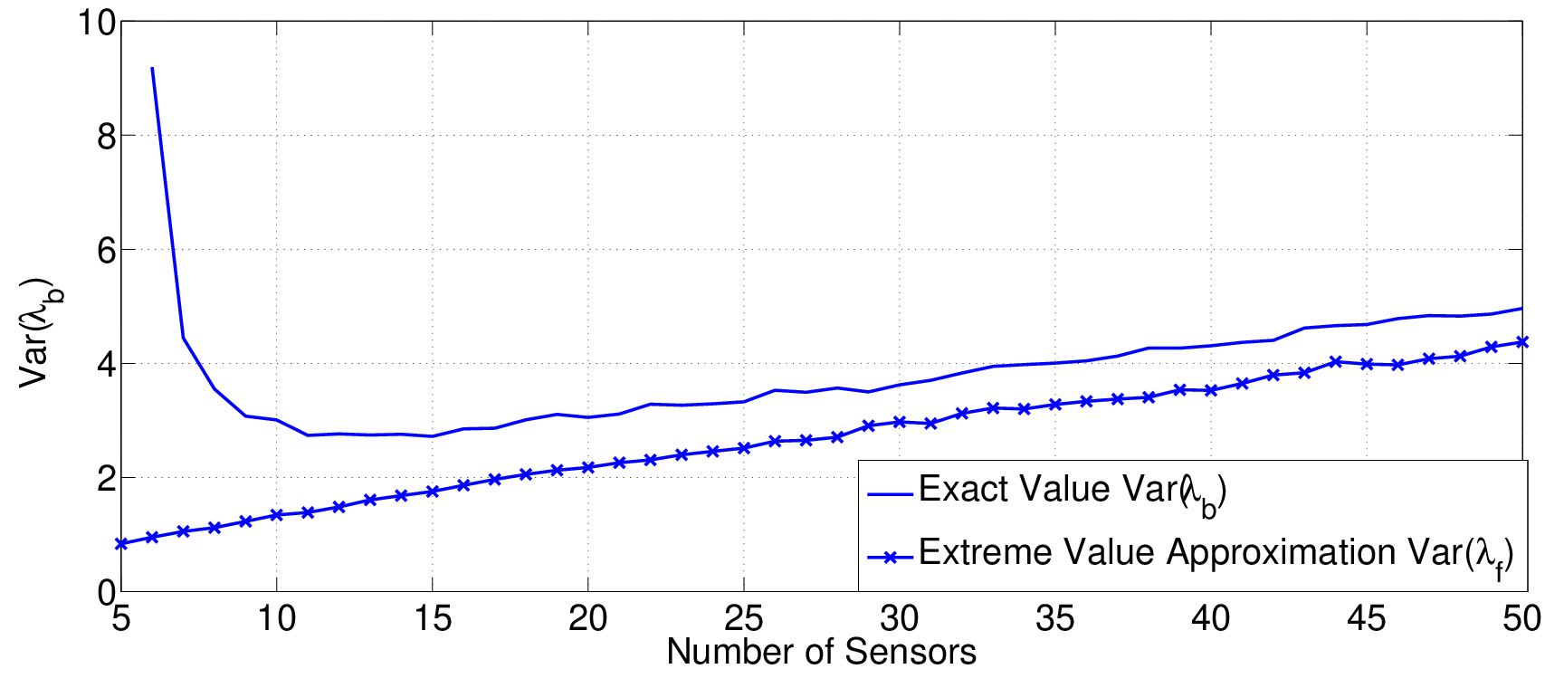
Figure 2 shows the variance with a similar setup. As seen, may be considered in practice as a good approximate value especially for a high number of sensors, where the relative error decreases.
For the case of fixed we calculated and by another MC experiment. We compared two different choices of DOA separation, namely and , both with unit coherent amplitudes. A single snapshot was considered and the SNR and were set to dB and respectively.
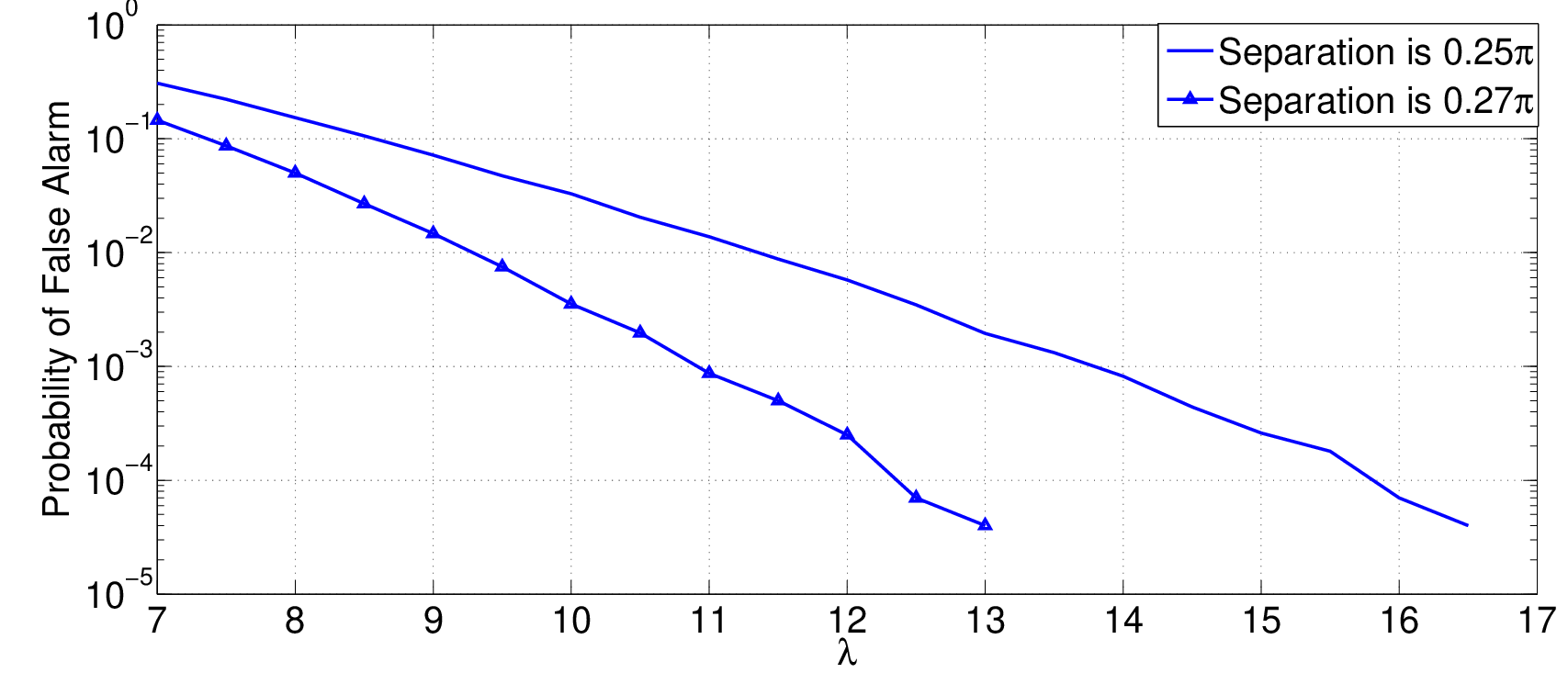
Figure 3 shows the resulting average PFA for different values of over realizations. As seen, better separated sources need smaller value of to achieve a required PFA.

Then, Figure 4 shows the trade-off between and in the above scenarios. As seen, the error dramatically decreases by increasing the separation. Reaching to the separation of , the error practically approaches the Cramer-Rao bound in the desirable range of . The same trend is observed when the number of sensors increases from to .
V-B Comparison with Other Methods
We finally compared the LASSO performance to that of ML (see (2)) with exhaustive search [46] and Conventional BeamForming (CBF) [49]. Figures 5 and 6 compare the estimate Mean Squared Errors and variances of three different estimators; CLASS, ML and CBF, respectively. The setup is similar to the one in Figures 2 and 3, while the number of sensors is fixed to 15. The results are the average of the outcomes of 100 trials at each noise level. We see that while the asymptotic variances of CLASS and ML methods coincide, the CLASS estimator has a higher asymptotic MSE. We conclude that CLASS modifies the solution of ML mostly by adding a bias term in the very high SNR regime. However, as SNR decreases, the MSE of CLASS reaches the one for the ML estimator in the SNR regime between -2 and 5 dBs. There is a significant (almost 3 dB) difference between threshold edge of LASSO and ML. Note that ML with exhaustive search is not practical and the difference might be less with a more realistic implementation.


VI Concluding Remarks
This work was devoted to analysis of LASSO as a non-linear estimator of a parametric signal. The main idea here was to parametrize the support, which brought a parametric interpretation of LASSO. To meet the continuous estimation requirements, the parametric LASSO was modified to CLASS. This is similar in nature to the approach in [37]. The parametric CLASS estimates were then analyzed by linearization in a high-SNR case and related to the original estimates by LASSO. The numerical implementation of CLASS was out of the scope of the current work. However, [37] also provides a CLASS implementation for a specific case, which we employed for numerical validation.
The above approach enabled to analyze LASSO more deeply from a deterministic point of view, which is of a great interest in applications, where LASSO is utilized to estimate parameters, such as radar localization. Although, important properties of LASSO, especially the role of the RP, presented in a limited number of scenarios, the current work provides a framework for further investigations. The MSE calculations also provide a new insight to the role of the RP. With our approach, we were able to calculate MSE and the false alarm rate, which commonly characterize an estimator of varying order in the high-SNR case. The process of false alarms were more generally characterized, but we left a more accurate investigation for a future work.
The current theoretical and numerical results suggest that LASSO provides a good trade-off between error and PFA, under some considerations about resolution. This is verified for a fixed-RP scenario. However, we suspect that employing a thresholding scheme would reduce PFA more, thus further improving the properties of LASSO. However, the numerical implementation may be crucial for the performance, and should therefore be the subject of a future study.
Appendix A LASSO Topology on ADP space
This part includes the definition of distance between atomic decompositions. Despite its complex technical definition it implies a natural concept, which easily follows from the analysis of LASSO.
Definition 2.
(LASSO-topology)
a) Consider an irreducible decomposition and another arbitrary decomposition . Let be the ball at . Then, is said to be in neighborhood of if
- 1.
The balls cover all indexes of , i.e.
- 2.
For each interval at each time index , we have that
(46) - 3.
For each and the relation implies that there exists such that
(47)
b) Two arbitrary decompositions and are called similar and shown by if there exists an irreducible decomposition such that both and are in -neighborhood of .


Figure 7 illustrates the concept of neighborhood, where a decomposition is represented by a set of arrows, whose amplitudes show , while their position denote . As seen, the definition does not restrict the orders. Condition 1 guarantees that the elements of are concentrated around the elements of . Then, Condition 2 provides that leads to a close synthesis to through the model in (1). Finally, Condition 3 guarantees that the LASSO cost values in (7) for and are close.
Appendix B Proof of Theorem 2
The proof is based on the following elements:
- 1.
For a regular manifold, there exists a finite subset , such that the matrix is full rank.
- 2.
The order of the LASSO and CLASS estimates are always bounded by , i.e. the estimates are in .
- 3.
For any and , the set of all decompositions with an order smaller than and amplitudes smaller than , i.e. , is compact in the regular topology of fixed dimension.
- 4.
Define the synthesis function such that for any and the relation implies (1). Also define . Then and are continuous.
- 5.
- 6.
The function is convex and conic, i.e. for any observation sets and , we have that and .
Using the above, the proof is straightforward. Note that from Observation 1, for any the solution to the group-LASSO optimization as well as the noiseless optimization is in , where is a sufficiently large upper-bound on the amplitudes which only depends on . If is further bounded, then is a constant.
Now, assume conversely that the theorem does not hold. This means that there exists an such that for any of the values there exists , a dense grid and such that , but their corresponding group-LASSO solution is out of the neghborhood of any solution to the noiseless CLASS for . Since is bounded, there exists a fixed , such that . Now, from the second observation, we may assume without loss of generality that the sequence has a limit , since otherwise one may take a converging subsequence. But is also out of the neighborhood of any solution of noiseless CLASS. We finally show in the sequel that in fact is contrarily equal to a solution , which completes the proof.
To show that is a minimizer of noiseless CLASS, first note that is a continuous function over a compact set . Thus, it is uniformly continuous. This means that for each value there exists a such that implies that . Fix a and corresponding . Consider the noiseless CLASS solution of . As is dense, for each , there exists a such that . For sufficiently large , this implies that , which further implies that . Take the approximate on-grid estimate and define . Note that
| (49) |
where and the right-hand side of the inequality is the cost calculated at . On the other hand, for large
| (50) |
where is a proper upper bound for over time. This shows that
| (51) |
Note also that the group-LASSO in the parametric form (17) can also be written as
| s.t | |||
| (52) |
which can be simplified to
| (53) |
Consider, , and . Then, the optimal point in (52) and (53) is given by and respectively. Then,
| (54) |
The right hand side is the cost in (53) evaluated at . Then, using (49), we obtain that
| (55) |
Letting tend to infinity, we get that
| (56) |
Until now, we have found observations converging to such that is the noiseless-LASSO solutions of over , i.e . Note that from the continuity of and we have that and
| (57) |
Define . Then, tends to zero as tends to infinity. Then from observation 6,
| (58) |
The final observation is that vanishes as tends to infinity. To see this consider the set in observation 1 and note that for an arbitrary and a large there exists indexes such that . Define . As the set of full-rank matrices is open, can be selected such that is full rank. Then,
| (59) |
which tends to zero as vanishes and the pseudo inverse stays bounded in the neighborhood of . Finally as tends to zero, taking the limit of (58) and combining with (57) we conclude that.
| (60) |
which shows that is a minimizer of the noiseless CLASS.
Appendix C Proof of Theorem 3
First, note that for a regular manifold , the set
| (61) |
is compact. For any grid , define
| (62) |
Then there exists a value such that for every dense grid , the set is compact. Furthermore, for any value , there exists a value such that for every dense grid ,
| (63) |
where denotes the union of all closed neighborhoods of elements in . Note also that is compact.
Now, consider an arbitrary solution of the noiseless CLASS. Take a sequence of dense grids such that for all and . Then, clearly and thus it minimizes noiseless group-LASSO over . From Theorem 1, this means that there exists a sequence of dual vectors such that
| (64) |
Note that for any fixed and sufficiently large we have that . Thus, has a subsequence converging to a point . Then
| (65) |
since the choice of is arbitrary. clearly also satisfies the other condition in (64).
Conversely, suppose that there exists satisfying (64) for . Then, we show that is the global minimum of noiseless-CLASS. Take any other decomposition with . Take the grid . Note that taking the dual verifiers in , the conditions of Theorem 1 for the noiseless case is satisfied. Thus, a minimizer of noiseless LASSO for grid and input , which implies that .
Finally, let us prove convergence. Suppose conversely that taking , there exists a sequence of primal solutions with corresponding dual parameters to the group lasso with a perturbed input where , and over the dense grid, such that is not in a neighborhood of any dual vector of the noiseless CLASS solution. But since can be bounded in a compact set for large enough and due to Theorem 2, the sequences has a subsequence converging to and respectively. Since is distant from any dual solution of noiseless CLASS, the limit is so. But, it is simple to check that the conditions of the current theorem holds for , which implies that is a dual for . This shows contradiction and completes the proof.
Appendix D Proof of Theorem 4
First, let us explain part (a) with more details. Convergence means that:
For any there exists a such that if the grid is dense, and perturbations satisfy and the solution is in neighborhood of a noiseless solution such that then, the false alarms are in neighborhood of and and hold.
Now, to prove this, we follow the following steps:
- 1.
Suppose that minimizes for a certain choice of , and true parameters and is another non-optimal point. Then, there exists a constant depending only on true parameters such that
(66) - 2.
Consider and such that the solution of LASSO optimization with a dense grid , and is in -neighborhood of the noiseless (true) solution. Denote by the corresponding parameters to the optimal point of LASSO with the optimal cost . Then,
(67) - 3.
Consider the same setup as above and remember that and minimize . Take the optimization
s.t. (68) and note that it has a solution with only two active elements in each cloud. Take this solution and calcualte the original LASSO cost at this point. Then
(69) - 4.
- 5.
Now, if (a) is not correct then there exists a such that for any arbitrary there exists a exact case such that . Consider now that we get from (69) that
(71) which leads to and contradicts to the choice of . Thus, (a) holds.
- 6.
- 7.
Similar to step 1 if , then one can conclude that
(73) - 8.
Appendix E Proof of Theorem 5
For part (a), it is easy to plug (38) in Theorem 3 and check by direct calculation that (34) ensures optimality of the true parameters,
For (b), since is consistent the optimization
| s.t. | |||
| (74) |
is feasible and has solution . It is simple to see that from the KKT theorem can be written as
| (75) |
where is the set of all peaks of the spectrum , thus including , and are suitable dual parameters. This shows that is in the range space of consisting of as columns, i.e
| (76) |
Furthermore,
| (77) |
and
| (78) |
It is easy by direct calculation to show that (76),(77) and (78) may only hold if is equal to in (35) if and are replaced by their primed counterparts and the resulting is zero. Then, similar to part (a), the optimality condition directly leads to (37) which establishes pure consistency for .
Appendix F Proof of Theorem 6
a) By definition, can be written as
| (79) | |||||
Note that the term is linear in . Thus, where is a quadratic function of . Note that if the case is purely consistent the leading term in can be shown by calculation to be negative. Furthermore . Thus, has exactly one positive root , given by (40), and , leading to
| (80) |
b) The result follows from direct calculation and noting that . To see this follow the following steps
- 1.
Note that is conic function of noise, i.e. .
- 2.
Then,
(81) - 3.
Note that , since
(82) - 4.
Finally,
(83)
References
- [1] T. T.Wu, Y. F.Chen, T.Hastie, E.Sobel, and K.Lange, “Genome-wide association analysis by lasso penalized logistic regression,” Bioinformatics, vol. 25, pp. 714–721, Mar. 2009.
- [2] F.Parvaresh, H.Vikalo, S.Misra, and B.Hassibi, “Recovering sparse signals using sparse measurement matrices in compressed dna microarrays,” IEEE, J. Select. Topics Signal Processing, vol. 2, pp. 275–285, June 2008.
- [3] W.Tu and S.Sun, “Spatial filter selection with lasso for eeg classification,” in Advanced Data Mining and Applications, Chongqing, China, 2010, pp. 142–149.
- [4] H.Konno and H.Yamazaki, “Mean-absolute deviation portfolio optimization model and its applications to tokyo stock market,” Manage. Sci., vol. 37, pp. 519–531, May 1991.
- [5] H.Yao, P.Gerstoft, P. M.Shearer, and C.Mecklenbräuker, “Compressive sensing of the tohoku-oki mw 9.0 earthquake: Frequency-dependent rupture modes,” Geophys. Res. Lett., vol. 38, Oct. 2011.
- [6] R.Tibshirani, “Regression shrinkage and selection via the lasso,” J. Roy. Stat. Soc., Series B (Methodological), vol. 58, pp. 267–288, Jan. 1996.
- [7] S. S.Chen, D. L.Donoho, and M. A.Saunders, “Atomic Decomposition by Basis Pursuit,” SIAM J. Sci. Comput., vol. 20, no. 1, pp. 33–61, Dec. 1998.
- [8] J. J.Fuchs, “On the application of the global matched filter to doa estimation with uniform circular arrays,” IEEE Trans. Signal Processing, vol. 49, no. 4, pp. 702–709, Apr. 2001.
- [9] M.Figueiredo, R.Nowak, and S.Wright, “Gradient projection for sparse reconstruction: Application to compressed sensing and other inverse problems,” IEEE Select. Topic. Signal Processing, vol. 1, pp. 586–597, Dec. 2007.
- [10] H.Zou, “The adaptive lasso and its oracle properties,” J. Amer. Stat. Assoc., vol. 101, no. 476, pp. 1418–1429, 2006.
- [11] T.Park and G.Casella, “The bayesian lasso,” J. Amer. Stat. Assoc., vol. 103, pp. 681–686, 2008.
- [12] H.Zayyani, M.Babaie-Zadeh, and C.Jutten, “Bayesian pursuit algorithm for sparse representation,” in IEEE International Conference on Acoustics, Speech and Signal Processing, ICASSP, Taipei, Taiwan, Apr. 2009, pp. 1549 –1552.
- [13] S. G.Mallat and Z.Zhang, “Matching pursuits with time-frequency dictionaries,” IEEE Trans. Signal Processing, vol. 41, pp. 3397–3415, Dec. 1993.
- [14] J. A.Tropp and A. C.Gilbert, “Signal recovery from random measurements via orthogonal matching pursuit,” IEEE Trans. Inform. Theory, vol. 53, pp. 4655–4666, Dec. 2007.
- [15] B.Efron, T.Hastie, L.Johnstone, and R.Tibshirani, “Least angle regression,” Ann. Stat., vol. 32, pp. 407–499, Apr. 2004.
- [16] D.Needell and J. A.Tropp, “Cosamp: Iterative signal recovery from incomplete and inaccurate samples,” Elsevier, Appl. Comput. Harmon. Anal., vol. 26, pp. 301–321, May 2009.
- [17] M.Lustig, D.Donoho, and J. M.Pauly, “Sparse mri: The application of compressed sensing for rapid mr imaging,” Resonance Med. Mag., vol. 58, pp. 1182–1195, Dec. 2007.
- [18] J.Provost and F.Lesage, “The application of compressed sensing for photo-acoustic tomography,” Medical Imaging, IEEE Transactions on, vol. 28, no. 4, pp. 585–594, 2009.
- [19] Y. C.Eldar and M.Mishali, “Robust recovery of signals from a structured union of subspaces,” IEEE Trans. Inform. Theory, vol. 55, no. 11, pp. 5302–5316, 2009.
- [20] M.Mishali and Y. C.Eldar, “From theory to practice: Sub-nyquist sampling of sparse wideband analog signals,” IEEE J. Select. Topics Signal Processing, vol. 4, pp. 375–391, Apr. 2010.
- [21] J. A.Tropp, J. N.Laska, M. F.Duarte, J. K.Romberg, and R. G.Baraniuk, “Beyond nyquist: Efficient sampling of sparse bandlimited signals,” IEEE Trans. Inform. Theory, vol. 56, pp. 520–544, Jan. 2010.
- [22] D.Malioutov, M.Cetin, and A.Willsky, “Source localization by enforcing sparsity through a laplacian prior: an svd-based approach,” IEEE Workshop Stat. Signal Processing, pp. 573–576, Sept. 2003.
- [23] R. G.Baraniuk, “Compressive sensing [lecture notes],” IEEE Signal Processing Mag., vol. 24, pp. 118–121, July 2007.
- [24] M.Arigovindan, M.Suhling, P.Hunziker, and M.Unser, “Variational image reconstruction from arbitrarily spaced samples: A fast multiresolution spline solution,” IEEE Trans. Image Processing, vol. 14, pp. 450–460, Apr. 2005.
- [25] P.Milanfar, W. C.Karl, and A. S.Willsky, “A moment-based variational approach to tomographic reconstruction,” IEEE Trans. Image Processing, vol. 5, pp. 459–470, Mar. 1996.
- [26] M. A.Herman and T.Strohmer, “High-resolution radar via compressed sensing,” Signal Processing, IEEE Transactions on, vol. 57, no. 6, pp. 2275–2284, 2009.
- [27] P.Stoica, A.Jakobsson, and J.Li, “Matched-filter bank interpretation of some spectral estimators,” Signal Processing, vol. 66, no. 1, pp. 45–59, 1998.
- [28] P.Zhao and B.Yu, “On model selection consistency of lasso,” The Journal of Machine Learning Research, vol. 7, pp. 2541–2563, 2006.
- [29] D.Donoho, “Compressed sensing,” IEEE Trans. Inform. Theory, vol. 52, no. 4, pp. 1289 –1306, Apr. 2006.
- [30] E. J.Candès and Y.Plan, “Near-ideal model selection by minimization,” Ann. Stat., vol. 37, pp. 2145–2177, Oct. 2009.
- [31] E. J.Candes and Y.Plan, “A Probabilistic and RIPless Theory of Compressed Sensing,” IEEE Trans. Inform. Theory, vol. 57, no. 11, pp. 7235–7254, Nov. 2011.
- [32] S.Oymak, C.Thrampoulidis, and B.Hassibi, “The squared-error of generalized lasso: A precise analysis,” arXiv preprint arXiv:1311.0830, 2013.
- [33] E.Candes and C.Fernandez-Granda, “Towards a mathematical theory of super-resolution,” arXiv preprint arXiv:1203.5871, 2012.
- [34] G.Tang, B. N.Bhaskar, P.Shah, and B.Recht, “Compressive sensing off the grid,” in Communication, Control, and Computing (Allerton), 2012 50th Annual Allerton Conference on. IEEE, 2012, pp. 778–785.
- [35] Z.Ben-Haim and Y. C.Eldar, “The cramer-rao bound for sparse estimation,” arXiv preprint arXiv:0905.4378, 2009.
- [36] P.Stoica and A.Nehorai, “Performance study of conditional and unconditional direction-of-arrival estimation,” IEEE Trans. Acoust., Speech, Signal Processing, vol. 38, no. 10, pp. 1783–1795, 1990.
- [37] B. N.Bhaskar and B.Recht, “Atomic norm denoising with applications to line spectral estimation,” in Communication, Control, and Computing (Allerton), 2011 49th Annual Allerton Conference on. IEEE, 2011, pp. 261–268.
- [38] M. V.Ashkan Panahi, “Gridless compressive sensing,” in IEEEInt. Conf. Acoust. Speech, Signal Processing, 2014.
- [39] J.Li and P.Stoica, “Efficient mixed-spectrum estimation with applications to target feature extraction,” Signal Processing, IEEE Transactions on, vol. 44, no. 2, pp. 281–295, 1996.
- [40] J. A.Fessler and A. O.Hero, “Space-alternating generalized expectation-maximization algorithm,” Signal Processing, IEEE Transactions on, vol. 42, no. 10, pp. 2664–2677, 1994.
- [41] D. L.Donoho and M.Elad, “Optimally sparse representation in general (nonorthogonal) dictionaries via l1 minimization,” Proceedings of the National Academy of Sciences, vol. 100, no. 5, pp. 2197–2202, 2003.
- [42] L. L.Scharf, Statistical signal processing. Addison-Wesley Reading, MA, 1991, vol. 98.
- [43] P.Stoica and Y.Selen, “Model-order selection: a review of information criterion rules,” Signal Processing Magazine, IEEE, vol. 21, no. 4, pp. 36–47, 2004.
- [44] J.Rissanen, “A universal prior for integers and estimation by minimum description length,” The Annals of statistics, pp. 416–431, 1983.
- [45] P.Stoica and N.Arye, “Music, maximum likelihood, and cramer-rao bound,” Acoustics, Speech and Signal Processing, IEEE Transactions on, vol. 37, no. 5, pp. 720–741, 1989.
- [46] B.Ottersten, M.Viberg, P.Stoica, and A.Nehorai, “Exact and large sample ML techniques for parameter estimation and detection in array processing,” in Radar Array Processing, Haykin, Litva, and Shepherd, Eds. Berlin: Springer-Verlag, 1993, pp. 99–151.
- [47] M. R.Osborne, B.Presnell, and B.Turlach, “A new approach to variable selection in least squares problems,” 1999.
- [48] H.Zhu, G.Leus, and G. B.Giannakis, “Sparsity-cognizant total least-squares for perturbed compressive sampling,” Signal Processing, IEEE Transactions on, vol. 59, no. 5, pp. 2002–2016, 2011.
- [49] H.Krim and M.Viberg, “Two decades of array signal processing research: the parametric approach,” IEEE Signal Processing Mag., vol. 13, pp. 67 –94, July 1996.