SLAC–PUB–15269 UCLA/12/TEP/104 SU-ITP-12/24
CERN-PH-TH/2012-288
maximally supersymmetric
Yang-Mills theory
diverges at six loops
Zvi Bern,(1) John Joseph Carrasco,(2) Lance J. Dixon,(3)
Michael R. Douglas,(4,5)
Matt von Hippel(4)
and Henrik Johansson(6)
(1) Department of Physics and Astronomy, UCLA,
Los Angeles, CA 90095-1547, USA
(2) Stanford Institute for Theoretical Physics
and Department of Physics,
Stanford University, Stanford, CA 94305-4060, USA
(3) SLAC National Accelerator Laboratory,
Stanford University, Stanford, CA 94309, USA
(4) Simons Center for Geometry and Physics,
Stony Brook University,
Stony Brook NY 11794
(5) I.H.E.S, Bures-sur-Yvette, France 91440
(6) Theory Division, Physics Department, CERN, CH-1211 Geneva 23,
Switzerland
bern@ucla.edu , jjmc@stanford.edu , lance@slac.stanford.edu , mdouglas@scgp.stonybrook.edu , matthew.vonhippel@stonybrook.edu , henrik.johansson@cern.ch
Abstract
The connection of maximally supersymmetric Yang-Mills theory to the theory in six dimensions has raised the possibility that it might be perturbatively ultraviolet finite in five dimensions. We test this hypothesis by computing the coefficient of the first potential ultraviolet divergence of planar (large ) maximally supersymmetric Yang-Mills theory in , which occurs at six loops. We show that the coefficient is nonvanishing. Furthermore, the numerical value of the divergence falls very close to an approximate exponential formula based on the coefficients of the divergences through five loops. This formula predicts the approximate values of the ultraviolet divergence at loop orders in the critical dimension . To obtain the six-loop divergence we first construct the planar six-loop four-point amplitude integrand using generalized unitarity. The ultraviolet divergence follows from a set of vacuum integrals, which are obtained by expanding the integrand in the external momenta. The vacuum integrals are integrated via sector decomposition, using a modified version of the FIESTA program.
I Introduction
Recent years have seen impressive progress in computing scattering amplitudes in general gauge and gravity theories (see, for example, the recent reviews [1]). The progress has been especially great for maximally supersymmetric Yang-Mills theory (MSYM), a theory with sixteen supercharges whose version is super-Yang-Mills theory. One application has been to study the ultraviolet (UV) properties of both gauge and gravity theories. The all-loop ultraviolet finiteness of super-Yang-Mills theory in was established in the 1980’s [2]. In dimensions , explicit unitarity-based amplitude computations in MSYM in the 1990’s [3, 4] showed that its degree of convergence was a bit better than had been anticipated. The results suggested that the correct finiteness bound for MSYM in dimensions at loops is
| (1) |
This bound is consistent with all-loop ultraviolet finiteness in . The bound (1) has been confirmed to all loop orders [5] using harmonic superspace [6]. The case is an exception; at one loop the first divergence is in , not [7]. Interestingly, maximal supergravity follows precisely the same finiteness bound, at least through four loops [8, 9, 10].
An important remaining question is whether the bound is saturated or not; that is, whether the coefficient of the potential logarithmic divergence in the critical dimension is nonzero or not, for each loop order. On the one hand, if the theory contains some unknown or hidden symmetry, then the coefficient in could vanish, leading to a higher critical dimension than expected at some loop order. That is, at a loop order affected by the symmetry, the lowest dimension with an ultraviolet divergence would be surprisingly high. On the other hand, if the bound is saturated, it proves that no additional hidden symmetries exist that alter the degree of divergence — at least through the loop orders explored.
The only known reliable means for answering such a question is to explicitly evaluate the ultraviolet divergence of an appropriate on-shell multi-loop scattering amplitude in the expected critical dimension. Such a computation can be performed either within the large-, or planar, limit of the theory with gauge group , or for a general gauge group including all subleading terms in the expansion. We know from these computations [4, 8, 11, 12, 13] that the bound (1) is indeed saturated through at least five loops. Interestingly, certain subleading-in- terms (e.g. double-trace terms), do have an improved behavior at three loops and beyond [11, 14, 10]. In this paper, we will only consider the leading-color (planar) terms.
If the bound (1) is saturated, then eq. (1) implies that in a divergence should first appear at six loops. A primary purpose of this paper is to compute the coefficient of this divergence. The case of is especially interesting because this theory has a UV completion, the theory in . The theory has no Lagrangian description; rather its existence follows from arguments in string theory and M theory [15]. This connection suggests that UV divergences in could give us information about the theory [16]. Of course, a low-energy effective theory usually has UV divergences, and by itself this connection does not lead to constraints. However, the present example is somewhat unique in that the theory has neither a dimensionless coupling constant nor a preferred scale, so that seemingly different quantities turn out to be related nonperturbatively. For example, the Kaluza-Klein modes in , arising from the compactification of the theory on a circle, can also be identified with solitons in the gauge theory [17, 16, 18] (solutions corresponding to instantons in ).
In ref. [16] these aspects were discussed in the context of -duality of the super-Yang-Mills theory obtained by compactification of MSYM on a circle, which can also be thought of as compactification of the theory on a two-torus. In this construction -duality has a geometric origin as an exchange of the two sides of the torus. This argument can be re-expressed in terms, and UV divergences in can potentially violate the -duality. An alternative argument suggesting finiteness [18] is based on the soliton-Kaluza-Klein correspondence for the compactified theory in the phase where the gauge symmetry is broken by separating the multiple branes used in its construction. Although these arguments do not prove that there are no UV divergences, they do motivate the question. In the present paper we definitively answer the question, by computing the numerical coefficient of the potential divergence in planar MSYM at six loops.
We find that the bound (1) is indeed saturated for and ; that is, the divergence has a nonzero coefficient. Somewhat surprisingly, we also find that, through at least six loops, the numerical values of the leading-color planar critical-dimension divergences can be fit accurately to a simple exponential Ansatz. Although we do not understand the origin of this simple functional form, it does have useful consequences: It gives us additional confidence that we have correctly computed the six-loop divergence and that it is non-zero. Moreover, by extrapolating to higher-loop orders it allows us to predict the approximate numerical values of the divergences for in their critical dimensions. This result suggests that even outside of four dimensions, MSYM has a surprisingly simple structure, reflected in the simple pattern of ultraviolet divergences.
Until recently, a direct evaluation of the six-loop ultraviolet properties of MSYM would have been out of reach. However, a combination of advances has made it possible. Many breakthroughs in understanding the structure of integrands for multi-loop amplitudes now allow for a rather straightforward construction of the integrand for the six-loop four-point amplitude in planar MSYM [1]. In addition to the integrand construction presented here, two recent papers give the same integrands in [19, 20], albeit presented somewhat differently. Our construction is also valid for loop momenta spanning the full five dimensions. Well-developed techniques for extracting UV divergences from amplitudes [21, 22, 8, 13] then allow us to express the six-loop divergence in terms of a relatively small number of vacuum integrals. Furthermore, a set of integral consistency relations [23], related to integration by parts identities [24], allows us to reduce the number of integrals further. It also provides for nontrivial cross-checks on numerical evaluations of the integrals and an independent means for estimating numerical integration uncertainty.
The final integrals obtained, after imposing the consistency relations, are nevertheless quite challenging to evaluate analytically. Instead, we make use of the major advances in numerical integration techniques. A long-standing challenge of numerically evaluating Euclidean Feynman integrals has been addressed by a computational technique called sector decomposition [25], implemented in several software packages [26, 27, 28] including the FIESTA package [29], used here. To our knowledge, the sector decomposition technique has not previously been applied at such a high loop order. However, when applied to this problem it leads successfully to integrals that can be evaluated on a moderate size (1000 node) cluster in a few days.
The remainder of this paper is organized as follows. In section II we outline the derivation of the integrand. Section III describes the procedure for extracting the UV divergence from the amplitude in terms of a set of vacuum integrals. Section IV explains the sector decomposition method, and section V describes details of the numerical evaluation. In section VI we give our conclusions, and comment on the feasibility of evaluating the seven-loop integrals that might be required to check whether the coefficient of the first potential counterterm of supergravity vanishes.
II Constructing the integrand
Our study of the UV properties of the planar MSYM amplitude in begins by constructing the integrand of the six-loop four-point amplitude. Because we need the integrand in five dimensions, we must ensure that our construction is valid for loop momenta inhabiting five spacetime dimensions. (We can always take the external momenta to be four-dimensional, and assign helicities to the external gluons if desired.) The five-dimensional validity of the integrand is accomplished by verifying unitarity cuts in higher dimensions, which we have done on a large class of cuts. In addition, to extract the UV divergences, we prefer a local form for the integrand, in which the only denominator factors are standard Feynman propagators. To find the desired representation, we use generalized unitarity, a particularly effective general purpose refinement of the unitarity method [30]. (For recent reviews of this method see refs. [31].) Our form for the integrand differs somewhat from recent ones based on four-dimensional constructions [19, 20]. However, we have confirmed analytic agreement in any dimension with the form in ref. [20] (which is also known to agree with that in ref. [19]).
We will focus on the leading-color, planar contribution to the six-loop amplitude in gauge theory, which has the same color structure as the tree amplitude, up to overall factors of the number of colors, . The color-decomposed form of the planar contribution to the -loop four-point amplitude is,
| (2) |
where is an -loop color-ordered partial amplitude. The sum runs over non-cyclic permutations, , of the external legs. In this expression we have suppressed momentum and helicity labels, leaving only the indices identifying the external legs. This decomposition holds for any set of external particles from the full gauge supermultiplet.
We will not describe our construction of the six-loop amplitude in any detail; it is similar to the construction of the five-loop planar amplitude given in ref. [12]. Integrands of planar amplitudes in MSYM are relatively simple to obtain because dual conformal symmetry severely restricts their form [32, 33, 34, 12, 35]. Although dimensional regularization breaks dual conformal invariance, it does so mildly at the level of the integrand. Indeed, the integrands of loop amplitudes in planar MSYM are known to have the same simple properties under dual conformal transformation in dimensions (and likely in all dimensions ) as they have in four dimensions [36, 37, 38]. The only breaking of dual conformal invariance comes from the integration measure. This allows us to use dual conformal symmetry to guide the construction of the integrand, even outside of four dimensions.


We write the Ansatz for the six-loop planar amplitude as
| (3) |
where is the color-ordered tree amplitude and the Mandelstam invariants are and . For bookkeeping purposes we organize the integrand in terms of graphs with only cubic vertices. We incorporate any contact (four-point) interactions by including numerator terms that can potentially cancel propagators. Thus there is no loss of generality in using cubic graphs. We decompose the integrand as
| (4) |
The sum runs over a set of distinct planar cubic graphs, which contribute in all eight possible arrangements generated by the dihedral group (corresponding to symmetries of a square with corners labeled by the four external momenta). The dimension of the symmetry group leaving each diagram invariant is . At six loops, there are 68 non-vanishing topologically distinct graphs shown in Figs. 1 and 2. The product in the denominator of eq. (4) runs over the 19 internal Feynman propagators of each labeled graph. The numerators, of each integral are polynomials,
| (5) |
where the monomials depend only on Lorentz invariants constructed from the dual (loop) momenta for each diagram, and the are numerical coefficients (rational numbers) to be determined from various constraints.
As a first step, we require the monomials to have the proper weight under dual conformal transformations. To expose the dual conformal properties we use the standard [32] dual variables , with
| (6) |
where are the external momenta. As discussed in detail in ref. [12], a practical way of expressing the internal momenta of a diagram in terms of dual variables is to use an -particle cut, which divides the -loop amplitude into two tree amplitudes connected by cut legs. At six loops, we consider a seven-particle cut in the channel. The seven cut legs carry momenta . The six dual loop momenta are then defined by,
| (7) |
The key dual conformal properties follow from the behavior of the integrand under dual coordinate inversion, which maps
| (8) |
In four dimensions, dual conformal invariance requires that each term in the integrand scales as [32]
| (9) |
The integrands of planar MSYM in dimensions have been shown to transform in exactly the same fashion to all loop orders, at least for [37, 38]. This property is sufficient for our purposes, since we are mainly interested in the integrand in .

The -particle cuts can also be used to generate the complete list of graphs needed at six loops. One considers all possible sewings of two tree-level cubic graphs that appear in these cuts [12]. (We modify the procedure slightly compared to ref. [12] by including only diagrams with cubic vertices.) In principle there are dual conformal graphs with four- or higher-point vertices that are not generated by the product of tree graphs of the -particle cuts; however, all such potential contributions, including those not detectable in the -particle cuts, can be assigned to graphs with only cubic vertices by multiplying and dividing by appropriate propagators. The construction of the potential numerators of each graph is then accomplished conveniently using the dual-graph representation, which exposes the dual conformal properties more simply.
Given a dual graph in the sewing, we construct the possible monomials as products of dual-momentum invariants . We keep only those terms with the dual conformal scaling dictated by eq. (9). To determine the rational-number coefficients we use generalized unitarity. A large number of coefficients are easy to identify, essentially by inspection, because the corresponding unitarity cuts are so simple. In particular, contributions with either a two-particle cut or a box subdiagram can be written down immediately, following the discussion in refs. [3, 11].
In addition, many of the coefficients vanish. All but one of the vanishings can be identified using the observation of ref. [34] that when the external momenta are taken off-shell the integrals must be infrared-finite in four dimensions. The sole integral with a vanishing coefficient which cannot be identified in this way is the integral displayed in Fig. 12 of ref. [12]. It consists of two identical three-loop three-point integrals, containing only box subdiagrams, and connected to each other by one common external leg.
The unitarity cuts include a sum over states in the supermultiplet for each cut leg. For generic cuts, the state sums are straightforward to implement numerically in four or six dimensions [39, 37, 40]. We have evaluated all four-dimensional cuts that decompose the amplitude into a sum of products of three-, four- or five-point amplitudes, as well as a variety of cuts involving six-point amplitudes. These cuts suffice to uniquely determine all the . The two-particle cut [3] and “box cut” [11] are valid in dimensions; hence all contributions to the integrand that are visible in such cuts are valid in any number of dimensions. In addition, a rather non-trivial cut of our expression, shown in fig. 3, was computed previously [37] using the six-dimensional spinor-helicity formalism of ref. [41] and superspace of ref. [42]. Thus this cut is valid for . This provides a highly nontrivial confirmation that the integrands are valid in .
We have performed a variety of consistency checks on the integrand. The unitarity cuts offer highly nontrivial self-consistency checks, because the same monomial can be visible in multiple cuts. As already mentioned we compared our integrand result against that of ref. [20]. As a further non-trivial check we confirmed that the unphysical singularities described in ref. [43] all cancel.
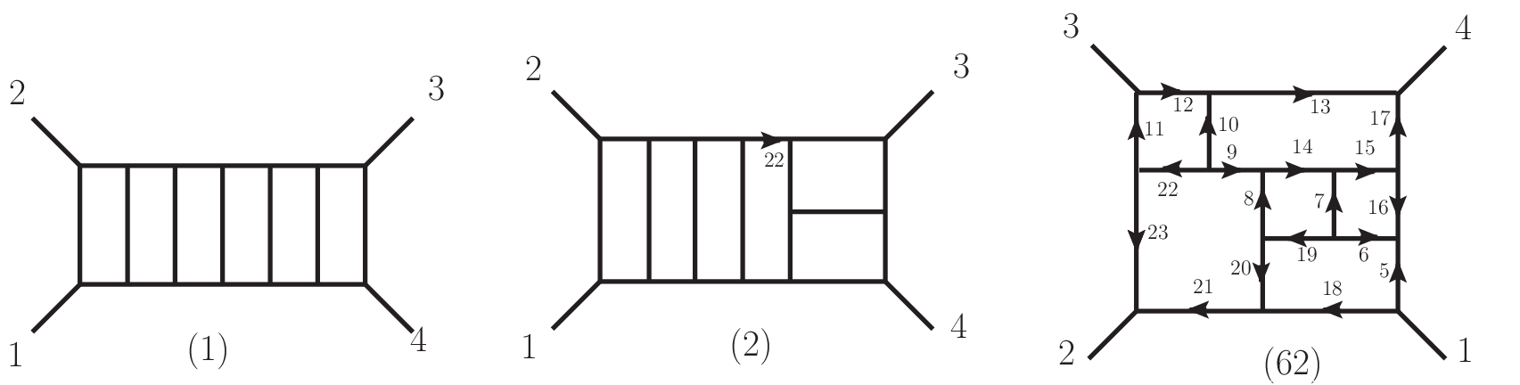
Some of the numerators are quite simple. For example, for the graphs labeled (1) and (2) in fig. 4, they are just
| (10) |
Other numerators are more complex. For example, the numerator of graph (62) with the labels in fig. 4 is
| (11) | |||||
In these expressions we have chosen labels that line up with the ones in the ancillary text file [44]. The symmetry factors of these graphs are , and . The complete sets of diagrams, numerators , and symmetry factors , are included in the ancillary file [44].
III From the amplitude to vacuum diagrams
Because the UV divergences arise from integration regions in which the loop momenta are parametrically much larger than the external momenta, extracting the UV divergences is a much simpler task than integrating the complete amplitude. We follow the same strategy as in our previous papers [8, 23, 10], based on Taylor expanding the integrands in small external momenta and then integrating the resulting vacuum integrals [21, 22]. The present case is relatively straightforward to analyze in the sense that the six-loop amplitude contains no subdivergences in , and because the expected overall divergence is manifestly logarithmic. However, the high loop order makes the loop integration for the vacuum integrals highly nontrivial.

III.1 Obtaining the vacuum diagrams
We consider the individual integrands appearing in eq. (4) in the limit of small external momenta , . We let , and then expand in the small parameter , keeping only the leading order. This reduces each to a sum over six distinct vacuum integrands,
| (12) |
where and are rational numbers determined by the expansion. (We will not list these coefficients separately for each diagram.) After the above vacuum integrands are integrated over the six loop momenta in , with the measure
| (13) |
we obtain six vacuum integrals, , shown in fig. 5. These integrals have numerator factors which are indicated to the left of each graph, and either one or two doubled propagator, whose location is indicated by a dot. The integrals contain no subdivergences; each integral has a single overall UV divergence in when all six loop momenta become large. Hence the integrals have only simple poles in .
Collecting the contributions from the 68 distinct integrals in the six-loop amplitude eq. (3), we obtain the following UV divergence
| (14) |
This simple expression for the divergence appears to be nonzero at first glance. However, we should expect that these six integrals are not independent so there may be cancellations among them. While all six integrals are positive definite after Wick rotation, enters with a coefficient of the opposite sign from the others. Thus no conclusion can be reached as to whether this expression vanishes or not without a careful analysis.
We begin the analysis by collecting all integrals under one common integration. By multiplying and dividing by propagators, all contributions can be brought to the form of the single vacuum graph displayed in fig. 6. Then by appropriately relabeling each term from the original to another set of loop momenta, all contributions can be rearranged to differ in only a single one-loop subintegral, indicated by the shaded region in fig. 6. The momenta are carried by the indicated one-loop subintegral. The momenta are the four momenta external to the one-loop box subintegral. In addition, we need two other independent loop momenta, which we take to be and , as indicated in fig. 6. Of these momenta, we take to be the six independent ones. In order to make the analysis easier, we may symmetrize the contributions over the automorphisms of the vacuum integral.

After appropriate relabelings, we can express the sum over all vacuum integrals as a single integral,
| (15) | |||||
where is the dimensional-regularization parameter and the vacuum “numerator” is
| (16) | |||||
using the momentum labels in fig. 6; that is, , , and . By a slight abuse of convention, we call this a numerator even though it is nonlocal. The numerator depends only on the momenta internal and external to the one-loop box subdiagram indicated by the shaded region in fig. 6.
Because of the minus sign in the last term — corresponding to in eq. (14) — it is easy to see that this integrand is not positive definite, even after Wick rotation. For example, for all terms but the last one vanish, making the integrand negative; and in the region where is much smaller than all other momentum invariants, the terms with factors will dominate, making the integrand positive. Thus, even after combining all contributions into a single integrand, there does not appear to be a simple way to determine the positivity, or vanishing, of the integral.
III.2 Simplifying the vacuum integrals via consistency relations
To simplify the expression further we need to identify relations between the different vacuum integrals. The integral identities that we need are related to integration-by-parts identities (IBP) [24], although they are only valid for the leading UV pole in the critical dimension, . These consistency relations [11] are obtained by demanding that different loop-momentum parameterizations of the integrals lead to the same final results. Using these relations we can both simplify the UV divergence, and give important cross-checks of the numerical evaluation. The latter use is particularly important, because the relations give independent estimates of the numerical uncertainties. The integral consistency relations also offer a potential path to finding a positive-definite expression for the divergence.
We now sketch a derivation of the consistency relations. For each of the 68 graphs describing the amplitude, we have simple relations from the shift invariance of the integrals,
| (17) |
for each , and , for , are the integrands of the distinct graphs. The are general numerator polynomials in the momentum invariants of the graphs. These polynomials are chosen to generate useful identities and are not the numerators of the amplitude. A judicious choice of a large set of will lead to a large set of linear relations for various vacuum integrals, which will include (but will not be limited to) the desired integrals . Below we describe such a judicious choice of numerators.
The identity (17) follows because the momentum dependence of the integrands is completely removed by a change of variables in the measure of eq. (17). In fact, eq. (17) is simply a statement that the integrals are reparametrization invariant under constant shifts.
Next we expand the integrands in small external momenta, , with a small parameter. In doing so, it is convenient to treat the integrands as belonging to equivalence classes controlled by the reparametrization freedom,
| (18) |
Expanding the two sides of eq. (18) in would not yield any nontrivial equations, only trivial reparametrization relations for vacuum integrals. However by combining the reparametrization freedom and the small momentum expansion, that is, by letting , we get nontrivial relations between different vacuum integrals,
| (19) |
where is an arbitrary integer-valued matrix, where different choices will generate different relations between vacuum integrals. The expansions in of the two different integrands will differ considerably. But by the reparametrization freedom, the two sides must be equivalent as integrands, or equal after integration. Therefore the various vacuum integrals that arise from integrating the coefficients of each element of in eq. (19) must satisfy nontrivial consistency relations.
It is important to make judicious choices for the integral numerators used to generate useful consistency relations. For example, using the original appearing in the integrand of the amplitude is not a good choice, because their divergences are manifestly logarithmic in . The UV divergence of a logarithmically-divergent integral is given by the leading term in . This term is always insensitive to the shift in the loop momenta , and so the available consistency relations become trivial. The first nontrivial relations are obtained using numerators containing one additional power of a loop momentum, which give linearly-divergent integrals in . The relevant vacuum integrals relations are obtained from the next-to-leading term in , which will differ on both sides of eq. (18). Numerators that give rise to quadratic divergences are also useful for extracting integral relations. However, numerators with an even higher degree are less helpful, since after taking derivatives with respect to they give rise to vacuum diagrams with three or more doubled propagators. These are outside the class of integrals that we are interested in; the vacuum diagrams in fig. 5 have at most two doubled propagators.
Furthermore, one should not choose that give rise to subdivergences in , because then the consistency relations may be contaminated by relations that are only valid for overlapping leading UV poles. Specifically, for integration in dimensions, UV subdivergences are possible in principle for two- and four-loop subdiagrams. Any generating such a subdivergence should be eliminated from the set of choices, because it will not produce any useful identities.

Generating a sufficient set of consistency relations then comes down to varying the polynomials for an appropriately large function space, without exceeding available computational resources. This includes varying the matrix that controls the reparametrization of the integrand, and then, as explained, expanding the integrals in small external momenta and demanding that the expansion is consistent for different choices of .
After generating about 1000 independent consistency relations, we found a much simpler three-term expression for the UV divergence of the planar six-loop four-point amplitudes. We then generated an additional 7000 consistency relations, and no further improvement was found. Thus a search for identities beyond the ones we found would probably be unfruitful, though we have not proven that they do not exist.

Using the derived consistency relations, the five tensor integrals can be reduced into eight scalar integrals with no loop momentum in the numerator, plus one relatively simple integral with only two powers of loop momentum in the numerator. One of the scalar integrals is from fig. 5. The eight new integrals are shown in fig. 7 and fig. 8. The most useful of the derived consistency relations are:
| (20) |

After applying the integral identities (20) to eq. (14), we obtain the following simplified form for the UV divergence,
| (21) |
Unfortunately, the coefficient of vacuum integral has a relative negative sign, so this simplified form is also not positive definite. One may wonder if there exists a different choice of basis of vacuum integrals that that allows the divergence to be expressed in a positive-definite form. While this possibility cannot be excluded by our analysis, we have not found such a representation, and it is quite likely that eq. (21) is the simplest integral basis decomposition.
IV Review of sector decomposition
Given that even the simplified form (21) still leaves open the question of whether the amplitude diverges in , and because analytic techniques are not yet powerful enough to cope with generic six-loop integrals, we have resorted to a numerical evaluation of the relevant vacuum integral using the method of sector decomposition. In this section we review this method, focusing on the salient features needed in our calculation.
If the amplitude under consideration is UV divergent, numerical evaluation with even a modest (say 5%) accuracy will suffice to prove it beyond any doubt. Indeed, here we shall provide such a numerical proof for MSYM in , settling the question of the potential finiteness of this theory. Even had it turned out finite, numerical analysis can provide important evidence in favor of this hypothesis. We are interested in the leading-logarithmic divergence of an integral with no subdivergences. After Feynman parametrization of the 15 propagators and integrating over the loop momentum, the overall divergence appears as a coefficient of a convergent -dimensional parametric integral. Eqs. (14) or (21) are fairly simple and it might seem to be an easy job to estimate it by Monte Carlo methods. If we estimate the integral as an average over uniformly distributed samples, we might imagine that the statistical uncertainty of such an estimate would be , where is the standard deviation of the integrand ( with the average value). An accuracy of would seem easily attainable.
However, the situation is more complex. The problem is that Feynman integrals in general, including eqs. (15) and (21), are not sufficiently convergent because of endpoint singularities. UV divergences in themselves are not a major problem, and are usually dealt with by subtracting a simpler integrand with the same divergent behavior. In the case at hand, even this is not necessary because the coefficient of the divergence is given by an (absolutely) convergent integral. However, the square of this integrand is not integrable. Because of this, the variance will diverge, and Monte Carlo estimation with the uniform measure has uncontrolled errors. In practice, it does not work.
IV.1 Sector decomposition overview
A straightforward way to deal with this problem is to carry out Monte Carlo integration with a sampling measure designed to overcome this problem. Let be the sampling measure. Then we rewrite
| (23) | |||||
where combines the original function with a change of measure factor. A particular case would be to take a new set of variables functionally related to , and to be uniform measure , in which case this factor would be the Jacobian for the change of variables. The error estimate for a Monte Carlo integral with this sampling measure is where is the new standard deviation,
| (24) |
where is the average value of . By reducing the variance, one can improve the accuracy of the Monte Carlo. In principle one could change variables to absorb all of the variation of into the measure to make constant, in which case the exact result would be obtained from a single sample. Of course, in practice such a change of variables would be prohibitively difficult.
For an integrand with power-like singularities, such as
| (25) |
we could use the change of variables , which absorbs the singularity into the measure and does not much complicate the integrand. The problem with applying this to a multi-dimensional Feynman integrand is that it has many different power-like singularities, arising from the many orders in which one can take the different parameters to zero.
The solution is to decompose the integration region into subregions or “sectors,” each of which has at most one singular behavior of this type. If we can do this, we can apply the change of variable eq. (25), or its multivariate generalization, to regularize the integral in each sector. While this approach was long used in formal proofs of perturbative renormalizability [45, 46, 47], it seems to have been first used in numerical integration by Binoth and Heinrich [25]. Since then has been implemented in several computer packages for numerically evaluating Feynman diagrams, starting with Bogner and Weinzierl [26] and including refs. [27, 28, 29]. Let us explain the basic ideas, leaving the details specific to our computation to section V.
We begin with an elementary example (from section 2 of ref. [48]), the two-dimensional integral
| (26) |
The form of the denominator makes the limit hard to control. Although in this simple example we could change variables to (say) and , this option will not be available for more complicated integrands.
Rather, we split the integration region into two parts, region 1 with and region 2 with . In region 1, we can make the change of variables
| (27) |
turning the integration region into . Similarly, in region 2 we take
| (28) |
again turning the integration region into a square. The integral becomes (suppressing the primes)
| (29) |
Now the nature of the singularity is manifest in the leading monomial terms, because the complicated denominator goes to in the singular region.
The same idea can be applied to a function of variables, call these with . The integration region is decomposed into subregions labeled by and defined by the inequality
| (30) |
In the ’th sector we redefine
| (31) |
to turn the subregion back into a unit cube. This will allow pulling out an overall singular behavior controlled by . Of course, the resulting integrand might still have a complicated singularity in the other variables. This must be dealt with by iterating the procedure and dividing the subregion into further subregions. Mathematically, this operation is called “blowing up” the singularity.
In these subsequent subdivisions, one need not include all variables in the blowup; one can instead take a subset of the variables and apply the same procedure. These choices might be used to simplify the result, or might even be needed in order for the procedure to terminate. The hope is that by choosing an appropriate sequence of these operations, one can find a finite set of subregions in each of which the integrand takes a simple form, as in eq. (29).
This procedure may be familiar to some readers from its use in algebraic geometry and string compactification, and the following remarks are addressed to them. In complex algebraic geometry, one can blow up an arbitrary point in an -dimensional space, replacing it with a . This is done by taking coordinates in which and applying the same changes of variables; the ’th subregion corresponds to the coordinate patch on in which we can take .
Suppose that the integrand is a rational function with denominator . The singularity is then the set of all points satisfying . Let us denote this singular set as . Since for a Feynman integrand the function is a polynomial, the set is by definition an algebraic variety, meaning the set of solutions of a system of polynomial equations. In fact it is a hypersurface, since we are setting a single polynomial to zero. In this context, a natural thing to try is to blow up the space containing , to a variety so that is nonsingular, meaning that it is defined locally by a single equation with . If we can do this, then the singular behavior of the integrand will simply be (or perhaps some power of this). By taking to be a local coordinate, we would accomplish our goal of realizing the singular behavior in a particularly simple form.
For present purposes, the main result of this mathematics is Hironaka’s theorem on resolution of singularities, which states that any singularity of an algebraic variety can be resolved (made nonsingular) by a succession of blowups. Furthermore, there are algorithms for concretely finding the resolution. Thus, we can use a blowup algorithm to resolve the singular locus , providing the multiparameter generalization of eq. (29).
While in ref. [26] this idea was used to give blowup algorithms which are guaranteed to terminate, these algorithms tend to produce a number of subregions which are exponential in the number of variables — this is perhaps natural as the number of orderings of variables is . This number of subregions would be computationally infeasible for . Bogner and Weinzierl [26] also proposed a simpler heuristic algorithm which, while not guaranteed to terminate, produces a simpler solution when it does. Another heuristic algorithm was proposed by Smirnov and Tentyukov [28], which we now describe.
IV.2 Heuristic sector decomposition
We recall from textbooks (e.g. ref. [49]) that the denominator of the Feynman integrand for a vacuum integral is the power of the Kirchoff polynomial of the graph,
| (32) |
where the sum is taken over the spanning trees of the graph . We are interested in the limiting behavior of as combinations of the variables go to zero. This behavior is encoded in its Newton polytope. Let be the degree of a monomial, considered as a vector in , so that
| (33) |
The Newton polytope of is the convex hull of the degrees of each of its terms; in other words, it is the set of all points in which can be obtained as linear combinations of these degrees with non-negative coefficients.
We need to desingularize each limit which takes a subset of the variables to zero. We now assume that is a polynomial with no constant term, so that every monomial in will go to zero for some such limits. However, many of the monomials are subleading and do not control any limit: if a monomial is the product of another monomial with a monomial of non-negative degree, it is subleading. In terms of the degrees, this requires
| (34) |
for every component.
We refer to the points which do not satisfy eq. (34) for any as the “low points” of the polytope. If the polytope has a single low point, then by factoring out the corresponding monomial, one obtains a polynomial with a nonzero constant term.
If there are multiple low points, we need to do a blowup. A blowup on a subset of the variables subdivides the current sector into sectors. In the ’th sector one applies the change of variables (31). This change of variables operates on the Newton polytope as
| (35) |
where is the vector whose components are for and for , and . We will then be able to factor out a common monomial; in other words shift the entire polytope in a way that keeps it in the upper quadrant. If the result includes the origin, we are done with this sector; otherwise we apply the same procedure recursively.
The next problem is to decide which subset of variables to involve in the blowup. The goal is to eliminate as many low points as possible; however it is better to leave the variables which do not contribute to this goal out of the blowup, in order to maximize the degree of the monomial that can be factored out. A condition on the subset which favors this is to project the polytope onto the subspace and require that the low points of the projected polytope linearly span this subspace. The heuristic algorithm is simply to choose, from the subsets satisfying this condition, the subset that has the largest value of .
This heuristic algorithm is too simple to desingularize general polynomials, including examples that are given in ref. [26]. If applied to these examples, it will go into an infinite loop.11 1 The “Strategy X” of ref. [26] and “Strategy S” of ref. [29] are somewhat more sophisticated and can handle these cases. However, the heuristic algorithm works for the class of polynomials in eq. (32); that is, scalar vacuum integrals with no doubled propagators. It also turns out to work for vacuum diagrams with no IR divergences and simple numerator factors, including the integrand (15). As observed in ref. [50], it works because it reproduces the results of a canonical sector decomposition procedure, which associates sectors with maximal forests [46, 47, 51]. While we leave the details for the references, a maximal forest is a hierarchical decomposition of the graph into a set of subgraphs satisfying certain conditions (each pair of subgraphs must obey one of the relations , or and can be disconnected by removing a single vertex). It can be shown that a maximal forest for a diagram with loops and edges contains trivial subgraphs (single lines) and nontrivial subgraphs, and the associated sector involves blowups each on distinct variables.
If the heuristic algorithm is reproducing this decomposition, then since every sector involves a succession of blowups on distinct variables, the algorithm is guaranteed to terminate with at most sectors. For and this is which is not much larger than the actual numbers we obtained. For and it is about .
V Numerical results and computational details
V.1 Numerical integration
There are several software packages for carrying out sector decomposition and subtraction of divergences, and for integrating the resulting expressions numerically [27, 28, 29]. We used the package FIESTA 2 [29], written in a combination of Mathematica [52] and C++ [53], and which can take advantage of multiple processors. However, a six-loop diagram is too complicated to evaluate directly. For example, the sector decomposition (which is not very parallelized) takes about a day per primary sector to run in Mathematica on a modern computer, and produces a total code for the integrands which takes up hundreds of gigabytes. Thus the computation must be split into smaller parts to make it feasible.
To do so, we only need a small portion of the FIESTA 2 software, and we have extracted this portion and adapted it to our purpose by hand. We did the sector decomposition on a small (10 node) cluster, and then performed the numerical integrations on a large (1000 node) cluster, using the adaptive quasi-Monte Carlo integrator Vegas [54]. An important element in FIESTA 2 is the CIntegrate package (see ref. [29], appendix F), which accepts a symbolic algebraic expression of the sort that can be produced easily by Mathematica, and compiles it into pseudocode that can be executed efficiently in C. Using this package, we were able to break down the computation by having Mathematica produce a file for each sector containing its integrand, which could be passed to a Vegas integration program. The integrals are of course completely independent, so this step is easy to parallelize. This approach also allowed us to keep the partial results for every sector, which helped in debugging and uncertainty analysis. The main cost was the need for 1–2 TB of disk storage, which is not large these days.
A rough estimate of the total running time can be obtained by multiplying the number of sectors (about here) by the time to integrate a sector, divided by the number of nodes. With a regular (low variance) integrand, the uncertainty as a function of the number of samples goes somewhere between for Monte Carlo and for quasi-Monte Carlo in low dimensions. Vegas did not need more than samples to achieve our requested relative precision of in any sector, and this took 2-3 seconds to do. Thus a million sector integration took less than an hour on the cluster.
There were a number of reasons that this success was not guaranteed from the start. Even once we knew that we had of order sectors, the next possible pitfall was that the integral might be small due to cancellations between larger results in individual sectors. The relative uncertainty of course depends strongly on the relative signs of the intermediate results; in the best case (a single sign) we might hope to gain a further statistical , while in the worst case the result might be comparable to the largest statistical uncertainty in a single sector (which could of course be improved by taking more samples) or even an uncontrolled systematic uncertainty. In fact, it appears that, at least in our computations, sector decomposition does lead to significant systematic uncertainties, as we will see below.

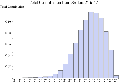
The actual situation is best judged by looking at the partial results, which we graph for diagram in fig. 10. There are sectors, all of which gave positive contributions. The same is manifestly true for and (since these integrands were positive), so there is no problem with cancellations.
Although a few sectors give anomalously large values, the largest sector value is only about times the average sector value, while the largest uncertainty is about times the overall standard deviation. One also sees that the distribution of sector integrals is roughly exponential except at the ends. This point is made in a different way in fig. 11. In this plot the sectors are listed in decreasing numerical order, with the graph showing the total contribution of each subset which has an exponentially growing number of sectors. Because the totals in each subset are roughly constant, this shows that the sector contributions decrease exponentially. Thus, while one cannot reduce the calculation to evaluating a smaller number of dominant sectors, there is structure which might be exploited to speed up the computation. For example, if one simply fits the distribution to an exponential and integrates that, one gets within of the actual total.
All this seems (at least naively) consistent with the uncertainties being entirely statistical, in which case it would be appropriate to add them in quadrature to get the statistical uncertainty estimate for integral of %. However, in previous use of sector decomposition, it has been observed that a purely statistical combination underestimates the true uncertainty. A more conservative estimate would be to treat the uncertainties as 100% correlated — what we will refer to as a “systematic” uncertainty estimate. In this case, we should add the uncertainties in every sector. For integral , this error is %.
In Table 1, we collect our results for the various vacuum integrals defined in section III, along with uncertainties that have been estimated by assuming 100% correlation among sectors. These results can be used to confirm the consistency relations (20); the degree of agreement is in turn a cross check of the integration uncertainties.
For example, consider the first equation in eq. (20). This relation evaluates to the numerical values
| (36) |
which is certainly acceptable and consistent with the systematic uncertainty hypothesis. The other consistency relations in eq. (20) work to a similar accuracy. Thus the combination of sector decomposition with the Vegas adaptive numerical integration appears to introduce systematic uncertainty, in the sense that the error is correlated between different sectors. Presumably this has to do with the modeling of the integrand at the sector boundaries.
Taking the uncertainties as 100% correlated and conservatively adding them directly (instead of in quadrature), the final result for the UV divergence is
| (37) | |||||
where
| (38) |
It is clear from this result that the coefficient of the UV divergence is nonzero, well within the integration uncertainty. This proves that MSYM is perturbatively ultraviolet divergent in .
| Integral | Value | Uncertainty | (Value) / |
|---|---|---|---|
| 1.3958 | 0.0043 | 5.05 | |
| 1.4522 | 0.0079 | 5.26 | |
| 1.3346 | 0.0069 | 4.83 | |
| 1.2643 | 0.0029 | 4.58 | |
| 1.1935 | 0.0026 | 4.32 | |
| 0.7631 | 0.0015 | 2.76 | |
| 0.8183 | 0.0024 | 2.96 | |
| 0.2762 | 0.0008 | 1 | |
| 0.5967 | 0.0012 | 2.16 | |
| 1.1490 | 0.0020 | 4.16 | |
| 1.1493 | 0.0019 | 4.16 | |
| 0.8391 | 0.0015 | 3.04 | |
| 1.8600 | 0.0028 | 6.74 | |
| 1.3755 | 0.0022 | 4.98 | |
| 0.9790 | 0.0017 | 3.55 |

V.2 Extrapolating in loop order
Maximally supersymmetric Yang-Mills four-point amplitudes have a smooth analytic behavior as a function of dimension, through at least six loops. As seen from their explicit forms the only dependence on the space-time dimension is in the loop momentum integration measure. Might this property lead somehow to a simple functional form describing the numerical values of the divergences in the critical dimensions, as a function of the number of loops ? To check this hypothesis, we plot the known values of the divergences in fig. 12 represented by the dots. In doing so we extract some simple overall factors, defining the numerical constant by
| (39) |
where is defined in eq. (38).
The value is not plotted because it does not obey the critical dimension bound given in eq. (1), and its divergence in differs kinematically from eq. (39) by a factor of :
| (40) |
The values of the divergences in from two through five loops have been given previously [4, 9, 10, 13]. Correcting a couple of overall signs, they are
| (41) |
where the expressions through are exact. The expression is approximate, but it is accurate to the digits given.
The linear behavior beyond in the upper panel of fig. 12 make clear that the coefficients of the divergences have an approximately exponential behavior. This observation motivates a simple Ansatz for the approximate form of the divergences at any loop order ,
| (42) |
The solid curve in the upper panel of fig. 12 is based on eq. (42) with the parameters
| (43) |
Interestingly, a nearly equally good fit is given by the following analytic form, which contains remarkably simple constants,
| (44) |
Since we do not know the precise functional form, for the purposes of extrapolating to higher-loop orders, it is useful to compare this to a different Ansatz,
| (45) |
where again , and are parameters. The dashed curve in fig. 12 corresponds to eq. (45) with the parameters
| (46) |
Before extrapolating to higher loops, an interesting exercise is to use eqs. (42) and (45) to see how well they predict (or rather postdict) the obtained UV divergences for . Because the Ansätze involves three parameters, we need to use the values for to fix the function. For the anstaz in eq. (42) we obtain
| (47) |
Plugging this solution into eq. (45) gives good predictions for the cases,
| (48) |
Similarly, for the Ansatz in eq. (45), we obtain
| (49) |
and
| (50) |
Presumably, the surprisingly good agreement between these approximate values and the calculated ones in eqs. (37) and (41) is somewhat accidental. Nevertheless it does illustrate the remarkably good predictive power of this simple extrapolation.
Using the fit parameters based on explicit results through six loops, we can easily predict approximate values for higher loops. For example, through from the Ansatz (42) we have,
| (51) |
while the Ansatz (45) gives
| (52) |
The small numerical integration uncertainty from our result feeds into this fit, propagating a few percent spread in the estimates. Of course, the functional forms may be too naive, but the two different fits gives an indication of the spread in predictions for such extrapolations.
Another interesting numerical observation from refs. [10, 13] is that for an gauge group, the ratio of the -suppressed subleading-color contributions to the leading color ones are fairly constant for and takes a value of about . This observation immediately gives us a prediction for the value of the divergence for the fully color-dressed amplitude (including nonplanar contributions),
| (53) | |||||
where and we assume that only the leading-color and -suppressed single-trace terms contribute, as is the case for .
It is interesting to note that, at least through four loops, the divergences of supergravity are in the same critical dimension , and they are proportional to the same linear combination of vacuum integrals as the -suppressed terms of MSYM [10, 55]. If this link between gravity and gauge theories were to persist to all loop orders, then the critical-dimension agreement alone would imply the four-dimensional ultraviolet finiteness of the theory. It would be very interesting to directly check these ultraviolet divergence patterns in both gauge and gravity theories at as high a loop order as possible, in order to see if they could give insight into the UV properties of supergravity, and into the precise values of the ultraviolet divergences in MSYM in , to all loop orders.
VI Conclusions and outlook
We have shown that planar MSYM diverges in at six loops, in accordance with expectations from previous explicit computations and supersymmetry arguments. This result raises various questions about its relation to theory as discussed in ref. [16]. Because (2,0) theory is superconformal, the MSYM UV cutoff must be related to the gauge coupling, and combining this relation with the -duality of the theory compactified to should lead to strong constraints. Probably the simplest next step is to work out the -dual extension of the two-loop amplitude.
Through five loops, the planar MSYM four-point integrand has a manifestly nonzero behavior in the terms that control the UV divergence in the expected critical dimension . Thus it is clear, without performing any loop integrals, that the amplitudes diverge in the critical dimension. At six loops, we were unable to find an integral representation in which all contributions are of the same sign. Therefore we had to explicitly evaluate nontrivial integrals in order to answer the question of whether MSYM diverges in . At six loops, practical analytic techniques are not available for generic integrals, so we resorted to numerical methods. In particular, we used the sector decomposition method as implemented in a modified version of the FIESTA program.
Our results show that, at least through six loops, the values of the ultraviolet divergences in the critical dimension of the planar amplitude approximately follow a simple exponential Ansatz. Indeed, extrapolating the results from two, three and four loops using this Ansatz matches the calculated values at five and six loops remarkably well. The fact that our calculated six-loop value closely matches this extrapolation gives us additional confidence that we have computed the six-loop divergence correctly. It also allows us to extrapolate the value of the divergences in the critical dimension to even higher loops. Moreover, as also noted in refs. [11, 13], the ratios of the numerical values of the -suppressed terms to the leading-color terms are approximately constant for . Assuming that this approximate constancy holds as well for gives us a definite prediction for the value of the subleading-color contributions to the divergence in . While the origin of the exponential behavior is still unclear, it does suggest that it might be possible to understand the ultraviolet divergences of MSYM in the critical dimension to all loop orders.
The same integration techniques described in this paper may be helpful for resolving other problems. An outstanding question that could be resolved by computation of a higher-loop divergence is whether and other supergravity theories might be perturbatively ultraviolet finite. (For recent reviews see refs. [56].) The current consensus for supergravity is that a potential counterterm valid under all known symmetries exists at seven loops [57, 58]. (A recent optimistic opinion for all orders finiteness may be found in ref. [59], while a pessimistic one may be found in ref. [60].) The same potential counterterm could be studied in at five loops, which should be well within reach of the types of integration techniques described here, once the supergravity integrand is constructed.
Intriguingly, through at least four loops, the explicit values of the supergravity divergences (in the same critical dimension as MSYM) are proportional to the same linear combination of vacuum integrals as enter the subleading-color divergence of theory at the same loop order. Moreover, half-maximal supergravity appears to be better behaved at three loops [61] than had been anticipated [58]. These results emphasize the need for further explicit computations at high loop orders, in order to help unravel the ultraviolet properties of supergravity theories. Our results demonstrate that evaluations of ultraviolet divergences are feasible through at least six loops. Due to the close relation between gravity and gauge-theory loop amplitudes [62], the results presented here also provide a concrete initial step towards determining the critical dimension of supergravity at six loops.
As yet, there are no explicit forms of the supergravity integrands beyond four loops, although recent progress in the nonplanar sector of MSYM at five loops [13] suggests that the four-point five-loop amplitude of supergravity is within reach. In any case, our success at six loops with the sector decomposition method suggests that although difficult, an evaluation of the integrals likely to occur at seven loops could be feasible. How hard would a numerical evaluation at seven loops be, along the lines discussed here? As we discussed, a reasonable guess for the number of sectors of a seven-loop integral is . If an integral takes 2 seconds, then a 1000-core cluster can evaluate these integrals in about 3 days. This is perhaps a bit slow as we might have hundreds of graphs and a more complex integrand, but with further optimization and a larger cluster even this computation should come within reach. It may also be possible to achieve further gains based on converting the vacuum integrals to propagator integrals and factorizing them into products of lower-loop integrals [21], as has been applied recently in maximally supersymmetric theories at four and five loops [10, 13]. There are also other methods for attacking this problem, such as the powerful DRA method [63], which offers much higher precision than can be obtained by sector decomposition, provided that an appropriate large system of linear equations can be solved symbolically.
In summary, in this paper we showed that maximally supersymmetric Yang-Mills theory diverges at six loops in , settling the question of whether the link to the theory might imply an improved UV behavior. We showed that, even at loop orders as high as six, and possibly higher, we can directly determine the UV properties of supersymmetric gauge and gravity theories. We also uncovered a simple approximate exponential pattern for the values of the divergences in the critical dimension where they first occur. This pattern may provide clues toward unraveling the all-loop-order UV structure. It is not obvious how to reconcile the appearance of a six-loop divergence in MSYM with the finiteness of its UV completion, the (2,0) theory in . Presumably, the divergence must be cutoff by additional degrees of freedom in the UV theory. As discussed in refs. [16, 18], there are already candidates for these degrees of freedom as nonperturbative states in the theory, so that it may be possible to understand this in terms. Perhaps the simplest conjecture is that -dual extensions of the amplitudes (as discussed in ref. [16]) are finite to all orders.
Acknowledgments
We thank Nima Arkani-Hamed, Radu Roiban and Edward Witten for helpful discussions. We also thank Paul Heslop and Gregory Korchemsky for assistance in comparing our amplitude integrand to their form [20]. We thank the Institute for Nuclear Theory in Seattle and the Banff International Research Station for hospitality, and Academic Technology Services at UCLA for computer support. This research was supported by the US Department of Energy under contracts DE–AC02–76SF00515 and DE–FG03–91ER40662. JJMC acknowledges that this publication was made possible through the support of the Stanford Institute for Theoretical Physics, and a grant from the John Templeton Foundation. The opinions expressed in this publication are those of the authors and do not necessarily reflect the views of the John Templeton Foundation.
References
- [1]
L. F. Alday and R. Roiban,
Phys. Rept. 468, 153 (2008)
[arXiv:0807.1889 [hep-th]];
R. Britto, J. Phys. A 44, 454006 (2011) [arXiv:1012.4493 [hep-th]];
J. M. Henn, J. Phys. A 44, 454011 (2011) [arXiv:1103.1016 [hep-th]];
Z. Bern and Y.-t. Huang, J. Phys. A 44, 454003 (2011) [arXiv:1103.1869 [hep-th]];
J. J. M. Carrasco and H. Johansson, J. Phys. A 44, 454004 (2011) [arXiv:1103.3298 [hep-th]];
T. Adamo, M. Bullimore, L. Mason and D. Skinner, J. Phys. A 44, 454008 (2011) [arXiv:1104.2890 [hep-th]];
L. J. Dixon, J. Phys. A 44, 454001 (2011) [arXiv:1105.0771 [hep-th]];
H. Ita, J. Phys. A 44, 454005 (2011) [arXiv:1109.6527 [hep-th]]. - [2]
S. Mandelstam,
Nucl. Phys. B 213, 149 (1983);
L. Brink, O. Lindgren and B. E. W. Nilsson, Phys. Lett. B 123, 323 (1983);
P. S. Howe, K. S. Stelle and P. K. Townsend, Nucl. Phys. B 214, 519 (1983). - [3] Z. Bern, J. S. Rozowsky and B. Yan, Phys. Lett. B 401, 273 (1997) [arXiv:hep-ph/9702424].
- [4] Z. Bern, L. J. Dixon, D. C. Dunbar, M. Perelstein and J. S. Rozowsky, Nucl. Phys. B 530, 401 (1998) [hep-th/9802162].
- [5] P. S. Howe and K. S. Stelle, Phys. Lett. B 554, 190 (2003) [hep-th/0211279].
- [6] A. Galperin, E. Ivanov, S. Kalitsyn, V. Ogievetsky and E. Sokatchev, Class. Quant. Grav. 1, 469 (1984); Class. Quant. Grav. 2, 155 (1985).
- [7] M. B. Green, J. H. Schwarz and L. Brink, Nucl. Phys. B 198, 474 (1982).
- [8]
Z. Bern, J. J. Carrasco, L. J. Dixon, H. Johansson, D. A. Kosower
and R. Roiban,
Phys. Rev. Lett. 98, 161303 (2007)
[arXiv:hep-th/0702112];
Z. Bern, J. J. M. Carrasco, L. J. Dixon, H. Johansson and R. Roiban, Phys. Rev. D 78, 105019 (2008) [arXiv:0808.4112 [hep-th]]. - [9] Z. Bern, J. J. M. Carrasco, L. J. Dixon, H. Johansson and R. Roiban, Phys. Rev. D 78, 105019 (2008) [arXiv:0808.4112 [hep-th]].
- [10] Z. Bern, J. J. M. Carrasco, L. J. Dixon, H. Johansson and R. Roiban, Phys. Rev. D 85, 105014 (2012) [arXiv:1201.5366 [hep-th]].
- [11] Z. Bern, J. J. M. Carrasco, L. J. Dixon, H. Johansson and R. Roiban, Phys. Rev. D 82, 125040 (2010) [arXiv:1008.3327 [hep-th]].
- [12] Z. Bern, J. J. M. Carrasco, H. Johansson and D. A. Kosower, Phys. Rev. D 76, 125020 (2007) [arXiv:0705.1864 [hep-th]].
- [13] Z. Bern, J. J. M. Carrasco, H. Johansson and R. Roiban, arXiv:1207.6666 [hep-th].
- [14]
N. Berkovits, M. B. Green, J. G. Russo and P. Vanhove,
JHEP 0911, 063 (2009)
[arXiv:0908.1923 [hep-th]];
G. Bossard, P. S. Howe and K. S. Stelle, Phys. Lett. B 682, 137 (2009) [arXiv:0908.3883 [hep-th]];
G. Bossard, P. S. Howe, U. Lindström, K. S. Stelle and L. Wulff, JHEP 1105, 021 (2011) [arXiv:1012.3142 [hep-th]]. - [15] E. Witten, in “Los Angeles 1995, Future perspectives in string theory”, pp. 501-523 [hep-th/9507121].
- [16] M. R. Douglas, JHEP 1102, 011 (2011) [arXiv:1012.2880 [hep-th]].
- [17]
M. Rozali,
Phys. Lett. B 400, 260 (1997)
[hep-th/9702136];
M. Berkooz, M. Rozali and N. Seiberg, Phys. Lett. B 408, 105 (1997) [hep-th/9704089];
N. Seiberg, Nucl. Phys. Proc. Suppl. 67, 158 (1998) [hep-th/9705117]. - [18] N. Lambert, C. Papageorgakis and M. Schmidt-Sommerfeld, JHEP 1101, 083 (2011) [arXiv:1012.2882 [hep-th]].
- [19] J. L. Bourjaily, A. DiRe, A. Shaikh, M. Spradlin and A. Volovich, JHEP 1203, 032 (2012) [arXiv:1112.6432 [hep-th]].
- [20] B. Eden, P. Heslop, G. P. Korchemsky and E. Sokatchev, Nucl. Phys. B 862, 450 (2012) [arXiv:1201.5329 [hep-th]].
- [21] A. A. Vladimirov, Theor. Math. Phys. 43, 417 (1980) [Teor. Mat. Fiz. 43, 210 (1980)].
- [22] N. Marcus and A. Sagnotti, Nuovo Cim. A 87, 1 (1985).
- [23] Z. Bern, J. J. Carrasco, L. J. Dixon, H. Johansson and R. Roiban, Phys. Rev. Lett. 103, 081301 (2009) [arXiv:0905.2326 [hep-th]].
- [24] K. G. Chetyrkin and F. V. Tkachov, Nucl. Phys. B 192, 159 (1981).
- [25] T. Binoth and G. Heinrich, Nucl. Phys. B 680, 375 (2004) [hep-ph/0305234].
- [26] C. Bogner and S. Weinzierl, Comput. Phys. Commun. 178, 596 (2008) [arXiv:0709.4092 [hep-ph]].
- [27] J. Carter and G. Heinrich, Comput. Phys. Commun. 182, 1566 (2011) [arXiv:1011.5493 [hep-ph]].
- [28] A. V. Smirnov and M. N. Tentyukov, Comput. Phys. Commun. 180, 735 (2009) [arXiv:0807.4129 [hep-ph]].
- [29] A. V. Smirnov, V. A. Smirnov and M. Tentyukov, Comput. Phys. Commun. 182, 790 (2011) [arXiv:0912.0158 [hep-ph]].
- [30]
Z. Bern, L. J. Dixon, D. C. Dunbar and D. A. Kosower,
Nucl. Phys. B 425, 217 (1994)
[arXiv:hep-ph/9403226];
Z. Bern, L. J. Dixon, D. C. Dunbar and D. A. Kosower, Nucl. Phys. B 435, 59 (1995) [arXiv:hep-ph/9409265]. - [31]
Z. Bern and Y.-t. Huang,
J. Phys. A 44, 454003 (2011)
[arXiv:1103.1869 [hep-th]];
J. J. M. Carrasco and H. Johansson, J. Phys. A 44, 454004 (2011) [arXiv:1103.3298 [hep-th]]. - [32] J. M. Drummond, J. Henn, V. A. Smirnov and E. Sokatchev, JHEP 0701, 064 (2007) [arXiv:hep-th/0607160].
- [33] Z. Bern, M. Czakon, L. J. Dixon, D. A. Kosower and V. A. Smirnov, Phys. Rev. D 75, 085010 (2007) [hep-th/0610248].
- [34] J. M. Drummond, G. P. Korchemsky and E. Sokatchev, Nucl. Phys. B 795, 385 (2008) [arXiv:0707.0243 [hep-th]].
- [35] N. Arkani-Hamed, J. L. Bourjaily, F. Cachazo, S. Caron-Huot and J. Trnka, JHEP 1101, 041 (2011) [arXiv:1008.2958 [hep-th]].
- [36] L. F. Alday, J. M. Henn, J. Plefka and T. Schuster, JHEP 1001, 077 (2010) [arXiv:0908.0684 [hep-th]].
- [37] Z. Bern, J. J. Carrasco, T. Dennen, Y.-t. Huang and H. Ita, Phys. Rev. D 83, 085022 (2011) [arXiv:1010.0494 [hep-th]].
- [38] T. Dennen and Y.-t. Huang, JHEP 1101, 140 (2011) [arXiv:1010.5874 [hep-th]].
- [39]
M. Bianchi, H. Elvang and D. Z. Freedman,
JHEP 0809, 063 (2008)
[arXiv:0805.0757 [hep-th]];
H. Elvang, D. Z. Freedman and M. Kiermaier, JHEP 0904, 009 (2009) [arXiv:0808.1720 [hep-th]];
J. M. Drummond, J. Henn, G. P. Korchemsky and E. Sokatchev, arXiv:0808.0491 [hep-th];
N. Arkani-Hamed, F. Cachazo and J. Kaplan, JHEP 1009, 016 (2010) [arXiv:0808.1446 [hep-th]]. - [40] Z. Bern, J. J. M. Carrasco, H. Ita, H. Johansson and R. Roiban, Phys. Rev. D 80, 065029 (2009) [arXiv:0903.5348 [hep-th]].
- [41] C. Cheung and D. O’Connell, JHEP 0907, 075 (2009) [arXiv:0902.0981 [hep-th]].
- [42] T. Dennen, Y.-t. Huang and W. Siegel, JHEP 1004, 127 (2010) [arXiv:0910.2688 [hep-th]].
- [43] F. Cachazo and D. Skinner, arXiv:0801.4574 [hep-th].
- [44] See the ancillary file of the arXiv version of this manuscript.
- [45] K. Hepp, Commun. Math. Phys. 2, 301 (1966).
- [46] E. R. Speer, Commun. Math. Phys. 23, 23 (1971) [Erratum-ibid. 25, 336 (1972)].
- [47] P. Breitenlohner and D. Maison, Commun. Math. Phys. 52, 11 (1977).
- [48] G. Heinrich, Int. J. Mod. Phys. A 23, 1457 (2008) [arXiv:0803.4177 [hep-ph]].
- [49] C. Itzykson and J.-B. Zuber, Quantum Field Theory, McGraw-Hill, New York, NY (1980).
- [50] A. V. Smirnov and V. A. Smirnov, JHEP 0905, 004 (2009) [arXiv:0812.4700 [hep-ph]].
- [51] V. A. Smirnov, Feynman integral calculus, Springer, Berlin, Germany (2006).
- [52] S. Wolfram, The Mathematica Book, 4th ed., Cambridge University Press, Cambridge, U.K. (1999).
- [53] B. Stroustrup, The C++ Programming Language, 3rd edition, Addison-Wesley, Reading, Mass. (1997).
- [54] T. Hahn, Comput. Phys. Commun. 168, 78 (2005) [hep-ph/0404043].
- [55] J. J. .Carrasco and H. Johansson, Phys. Rev. D 85, 025006 (2012) [arXiv:1106.4711 [hep-th]].
- [56]
Z. Bern, J. J. M. Carrasco and H. Johansson,
arXiv:0902.3765 [hep-th];
H. Nicolai, Physics 2, 70 (2009);
R. P. Woodard, Rept. Prog. Phys. 72, 126002 (2009) [arXiv:0907.4238 [gr-qc]];
L. J. Dixon, arXiv:1005.2703 [hep-th];
H. Elvang, D. Z. Freedman and M. Kiermaier, J. Phys. A 44, 454009 (2011) [arXiv:1012.3401 [hep-th]];
Z. Bern, J. J. Carrasco, L. Dixon, H. Johansson and R. Roiban, Fortsch. Phys. 59, 561 (2011) [arXiv:1103.1848 [hep-th]]. - [57]
M. B. Green, J. G. Russo and P. Vanhove,
JHEP 1006, 075 (2010)
[arXiv:1002.3805 [hep-th]];
J. Björnsson and M. B. Green, JHEP 1008, 132 (2010) [arXiv:1004.2692 [hep-th]];
R. Kallosh and P. Ramond, arXiv:1006.4684 [hep-th];
G. Bossard, C. Hillmann and H. Nicolai, JHEP 1012, 052 (2010) [arXiv:1007.5472 [hep-th]];
G. Bossard, P. S. Howe and K. S. Stelle, JHEP 1101, 020 (2011) [arXiv:1009.0743 [hep-th]];
N. Beisert, H. Elvang, D. Z. Freedman, M. Kiermaier, A. Morales and S. Stieberger, Phys. Lett. B 694, 265 (2010) [arXiv:1009.1643 [hep-th]];
J. Björnsson, JHEP 1101, 002 (2011) [arXiv:1009.5906 [hep-th]]. - [58] G. Bossard, P. S. Howe, K. S. Stelle and P. Vanhove, Class. Quant. Grav. 28, 215005 (2011) [arXiv:1105.6087 [hep-th]].
- [59] R. Kallosh, JHEP 1203, 083 (2012) [arXiv:1103.4115 [hep-th]].
- [60] T. Banks, arXiv:1205.5768 [hep-th].
- [61]
Z. Bern, S. Davies, T. Dennen and Y.-t. Huang,
Phys. Rev. Lett. 108, 201301 (2012)
[arXiv:1202.3423 [hep-th]];
P. Tourkine and P. Vanhove, Class. Quant. Grav. 29, 115006 (2012) [arXiv:1202.3692 [hep-th]]. - [62] Z. Bern, J. J. M. Carrasco and H. Johansson, Phys. Rev. Lett. 105, 061602 (2010) [arXiv:1004.0476 [hep-th]].
- [63]
R. N. Lee,
Nucl. Phys. B 830, 474 (2010)
[arXiv:0911.0252 [hep-ph]];
R. N. Lee, A. V. Smirnov and V. A. Smirnov, Eur. Phys. J. C 71, 1708 (2011) [arXiv:1103.3409 [hep-th]]; Nucl. Phys. B 856, 95 (2012) [arXiv:1108.0732 [hep-th]];
R. N. Lee and V. A. Smirnov, arXiv:1209.0339 [hep-ph].