Graph Estimation From Multi-attribute Data
Abstract
Many real world network problems often concern multivariate nodal attributes such as image, textual, and multi-view feature vectors on nodes, rather than simple univariate nodal attributes. The existing graph estimation methods built on Gaussian graphical models and covariance selection algorithms can not handle such data, neither can the theories developed around such methods be directly applied. In this paper, we propose a new principled framework for estimating graphs from multi-attribute data. Instead of estimating the partial correlation as in current literature, our method estimates the partial canonical correlations that naturally accommodate complex nodal features. Computationally, we provide an efficient algorithm which utilizes the multi-attribute structure. Theoretically, we provide sufficient conditions which guarantee consistent graph recovery. Extensive simulation studies demonstrate performance of our method under various conditions. Furthermore, we provide illustrative applications to uncovering gene regulatory networks from gene and protein profiles, and uncovering brain connectivity graph from functional magnetic resonance imaging data.
Keywords: Graphical model selection; Multi-attribute data; Network analysis; Partial canonical correlation.
1 Introduction
In many modern problems, we are interested in studying a network of entities with multiple attributes rather than a simple univariate attribute. For example, when an entity represents a person in a social network, it is widely accepted that the nodal attribute is most naturally a vector with many personal information including demographics, interests, and other features, rather than merely a single attribute, such as a binary vote as assumed in the current literature of social graph estimation based on Markov random fields (Banerjee et al., 2008, Kolar et al., 2010). In another example, when an entity represents a gene in a gene regulation network, modern data acquisition technologies allow researchers to measure the activities of a single gene in a high-dimensional space, such as an image of the spatial distribution of the gene expression, or a multi-view snapshot of the gene activity such as mRNA and protein abundances, rather than merely a single attribute such as an expression level, which is assumed in the current literature on gene graph estimation based on Gaussian graphical models (Peng et al., 2009). Indeed, it is somewhat surprising that existing research on graph estimation remains largely blinded to the analysis of multi-attribute data that are prevalent and widely studied in the network community. Existing algorithms and theoretical analysis relies heavily on covariance selection using graphical lasso, or penalized pseudo-likelihood. They can not be easily extended to graphs with multi-variate nodal attributes.
In this paper, we present a study on graph estimation from multi-attribute data, in an attempt to fill the gap between the practical needs and existing methodologies from the literature. Under a Gaussian graphical model, one assumes that a -dimensional random vector follows a multivariate Gaussian distribution with the mean and covariance matrix , with each component of the vector corresponding to a node in the graph. Based on independent and identically distributed observations, one can estimate an undirected graph , where the node set corresponds to the variables, and the edge set describes the conditional independence relationships among the variables, that is, variables and are conditionally independent given all the remaining variables if . Given multi-attribute data, this approach is clearly invalid, because it naively translates to estimating one graph per attribute. A subsequent integration of all such graphs to a summary graph on the entire dataset may lead to unclear statistical interpretation.
We consider the following new setting for estimating a multi-attribute graph. In this setting, we consider a “stacked” long random vector where are themselves random vectors that jointly follow a multivariate Gaussian distribution with mean and covariance matrix , which is partitioned as
| (1) |
with . Without loss of generality, we assume . Let be a graph with the vertex set and the set of edges that encodes the conditional independence relationships among . That is, each node of the graph corresponds to the random vector and there is no edge between nodes and in the graph if and only if is conditionally independent of given all the vectors corresponding to the remaining nodes, . Such a graph is also known as a Markov network (of Markov graph), which we shall emphasize in this paper to compare with an alternative graph over known as the association network, which is based on pairwise marginal independence. Conditional independence can be read from the inverse of the covariance matrix, as the block corresponding to and will be equal to zero. Let be a sample of independent and identically distributed vectors drawn from . For a vector , we denote the component corresponding to the node . Our goal is to estimate the structure of the graph from the sample . Note that we allow for different nodes to have different number of attributes, which is useful in many applications, e.g., when a node represents a gene pathway in a regulatory network.
Using the standard Gaussian graphical model for univariate nodal observations, one can estimate the Markov graph for each attribute individually by estimating the sparsity pattern of the precision matrix . This is also known as the covariance selection problem (Dempster, 1972). For high dimensional problems, Meinshausen and Bühlmann (2006) propose a parallel Lasso approach for estimating Gaussian graphical models by solving a collection of sparse regression problems. This procedure can be viewed as a pseudo-likelihood based method. In contrast, Banerjee et al. (2008), Yuan and Lin (2007), and Friedman et al. (2008) take a penalized likelihood approach to estimate the sparse precision matrix . To reduce estimation bias, Lam and Fan (2009), Johnson et al. (2012), and Shen et al. (2012) developed the non-concave penalties to penalize the likelihood function. More recently, Yuan (2010) and Cai et al. (2011) proposed the graphical Dantzig selector and CLIME, which can be solved by linear programming and are more amenable to theoretical analysis than the penalized likelihood approach. Under certain regularity conditions, these methods have proven to be graph estimation consistent (Ravikumar et al., 2011, Yuan, 2010, Cai et al., 2011) and scalable software packages, such as and , were developed to implement these algorithms (Zhao et al., 2012). However, in the case of multi-attribute data, it is not clear how to combine estimated graphs to obtain a single Markov graph reflecting the structure of the underlying complex system. This is especially the case when nodes in the graph contain different number of attributes.
In a previous work, Katenka and Kolaczyk (2011) proposed a method for estimating association networks from multi-attribute data using canonical correlation as a dependence measure between two groups of attributes. However, association networks are known to confound the direct interactions with indirect ones as they only represent marginal associations. In contrast, we develop a method based on partial canonical correlation, which give rise to a Markov graph that is better suited for separating direct interactions from indirect confounders. Our work is related to the literature on simultaneous estimation of multiple Gaussian graphical models under a multi-task setting (Guo et al., 2011, Varoquaux et al., 2010, Honorio and Samaras, 2010, Chiquet et al., 2011, Danaher et al., 2011). However, the model given in (1) is different from models considered in various multi-task settings and the optimization algorithms developed in the multi-task literature do not extend to handle the optimization problem given in our setting.
Unlike the standard procedures for estimating the structure of Gaussian graphical models (e.g., neighborhood selection (Meinshausen and Bühlmann, 2006) or glasso (Friedman et al., 2008)), which infer the partial correlations between pairs of multi-attribute nodes, our proposed method estimates the partial canonical correlations between pairs of nodes, which leads to a graph estimator over multi-attribute nodes that bears the same probabilistic independence interpretations as that of the graph from Gaussian graphical model over univariate nodes. Under this new framework, the contributions of this paper include: (i) Computationally, an efficient algorithm is provided to estimate the multi-attribute Markov graphs; (ii) Theoretically, we provide sufficient conditions which guarantee consistent graph recovery; and (iii) Empirically, we apply our procedure to uncover gene regulatory networks from gene and protein profiles, and to uncover brain connectivity graph from functional magnetic resonance imaging data.
2 Methodology
In this section, we propose to estimate the graph by estimating non-zero partial canonical correlation between the nodes. This leads to a penalized maximum likelihood objective, for which we develop an efficient optimization procedure.
2.1 Preliminaries
Let and be two multivariate random vectors. Canonical correlation is defined between and as
That is, computing canonical correlation between and is equivalent to maximizing the correlation between two linear combinations and with respect to vectors and . Canonical correlation can be used to measure association strength between two nodes with multi-attribute observations. For example, in Katenka and Kolaczyk (2011), a graph is estimated from multi-attribute nodal observations by elementwise thresholding the canonical correlation matrix between nodes, but such a graph estimator may confound the direct interactions with indirect ones.
In this paper, we exploit the partial canonical correlation to estimate a graph from multi-attribute nodal observations. A graph is going to be formed by connecting nodes with non-zero partial canonical correlation. Let and , then the partial canonical correlation between and is defined as
| (2) |
that is, the partial canonical correlation between and is equal to the canonical correlation between the residual vectors of and after the effect of is removed (Rao, 1969).
Let denote the precision matrix under the model in (1). Using standard results for the multivariate Gaussian distribution (see also Equation (7) in Rao (1969)), a straightforward calculation shows that11 1 Calculation given in Appendix C.3
| (3) |
This implies that estimating whether the partial canonical correlation is zero or not can be done by estimating whether a block of the precision matrix is zero or not. Furthermore, under the model in (1), vectors and are conditionally independent given if and only if partial canonical correlation is zero. A graph built on this type of inter-nodal relationship is known as a Markov graph, as it captures both local and global Markov properties over all arbitrary subsets of nodes in the graph, even though the graph is built based on pairwise conditional independence properties. In 2.2, we use the above observations to design an algorithm that estimates the non-zero partial canonical correlation between nodes from data using the penalized maximum likelihood estimation of the precision matrix.
Based on the relationship given in (3), we can motivate an alternative method for estimating the non-zero partial canonical correlation. Let denote the set of all nodes minus the node . Then
Since , we observe that a zero block can be identified from the regression coefficients when each component of is regressed on . We do not build an estimation procedure around this observation, however, we note that this relationship shows how one would develop a regression based analogue of the work presented in Katenka and Kolaczyk (2011).
2.2 Penalized Log-Likelihood Optimization
Based on the data , we propose to minimize the penalized negative Gaussian log-likelihood under the model in (1),
| (4) |
where is the sample covariance matrix, denotes the Frobenius norm of and is a user defined parameter that controls the sparsity of the solution . The Frobenius norm penalty encourages blocks of the precision matrix to be equal to zero, similar to the way that the penalty is used in the group Lasso (Yuan and Lin, 2006). Here we assume that the same number of samples is available per attribute. However, the same method can be used in cases when some samples are obtained on a subset of attributes. Indeed, we can simply estimate each element of the matrix from available samples, treating non-measured attributes as missing completely at random (Kolar and Xing, 2012, for more details see).
The dual problem to (4) is
| (5) |
where is the dual variable to and denotes the determinant of . Note that the primal problem gives us an estimate of the precision matrix, while the dual problem estimates the covariance matrix. The proposed optimization procedure, described below, will simultaneously estimate the precision matrix and covariance matrix, without explicitly performing an expensive matrix inversion.
We propose to optimize the objective function in (4) using an inexact block coordinate descent procedure, inspired by Mazumder and Agarwal (2011). The block coordinate descent is an iterative procedure that operates on a block of rows and columns while keeping the other rows and columns fixed. We write
and suppose that are the current estimates of the precision matrix and covariance matrix. With the above block partition, we have . In the next iteration, is of the form
and is obtained by minimizing
| (6) |
Exact minimization over the variables and at each iteration of the block coordinate descent procedure can be computationally expensive. Therefore, we propose to update and using one generalized gradient step update (see Beck and Teboulle (2009)) in each iteration. Note that the objective function in (6) is a sum of a smooth convex function and a non-smooth convex penalty so that the gradient descent method cannot be directly applied. Given a step size , generalized gradient descent optimizes a quadratic approximation of the objective at the current iterate , which results in the following two updates
| (7) | ||||
| (8) |
If the resulting estimator is not positive definite or the update does not decrease the objective, we halve the step size and find a new update. Once the update of the precision matrix is obtained, we update the covariance matrix . Updates to the precision and covariance matrices can be found efficiently, without performing expensive matrix inversion, as we show in Appendix A (see (11)–(13)). Combining all three steps we get the following algorithm:
- 1.
Set the initial estimator and . Set the step size .
- 2.
For each perform the following:
- 3.
Repeat Step 2 until the duality gap
where is a prefixed precision parameter (for example, ).
Finally, we form a graph by connecting nodes with .
Computational complexity of the procedure is given in Appendix B. Convergence of the above described procedure to the unique minimum of the objective function in (4) does not follow from the standard results on the block coordinate descent algorithm (Tseng, 2001) for two reasons. First, the minimization problem in (6) is not solved exactly at each iteration, since we only update and using one generalized gradient step update in each iteration. Second, the blocks of variables, over which the optimization is done at each iteration, are not completely separable between iterations due to the symmetry of the problem. The proof of the following convergence result is given in Appendix C.
2.3 Efficient Identification of Connected Components
When the target graph is composed of smaller, disconnected components, the solution to the problem in (4) is block diagonal (possibly after permuting the node indices) and can be obtained by solving smaller optimization problems. That is, the minimizer can be obtained by solving (4) for each connected component independently, resulting in massive computational gains. We give necessary and sufficient condition for the solution of (4) to be block-diagonal, which can be easily checked by inspecting the empirical covariance matrix .
Our first result follows immediately from the Karush-Kuhn-Tucker conditions for the optimization problem (4) and states that if is block-diagonal, then it can be obtained by solving a sequence of smaller optimization problems.
Lemma 2.
If the solution to (4) takes the form , that is, is a block diagonal matrix with the diagonal blocks , then it can be obtained by solving
separately for each , where are submatrices of corresponding to .
Next, we describe how to identify diagonal blocks of . Let be a partition of the set and assume that the nodes of the graph are ordered in a way that if , , , then . The following lemma states that the blocks of can be obtained from the blocks of a thresholded sample covariance matrix.
Lemma 3.
A necessary and sufficient conditions for to be block diagonal with blocks is that for all , , .
Blocks can be identified by forming a matrix with elements and computing connected components of the graph with adjacency matrix . The lemma states also that given two penalty parameters , the set of unconnected nodes with penalty parameter is a subset of unconnected nodes with penalty parameter . The simple check above allows us to estimate graphs on datasets with large number of nodes, if we are interested in graphs with small number of edges. However, this is often the case when the graphs are used for exploration and interpretation of complex systems. Lemma 3 is related to existing results established for speeding-up computation when learning single and multiple Gaussian graphical models (Witten et al., 2011, Mazumder and Hastie, 2012, Danaher et al., 2011). Each condition is different, since the methods optimize different objective functions.
3 Consistent Graph Identification
In this section, we provide theoretical analysis of the estimator described in 2.2. In particular, we provide sufficient conditions for consistent graph recovery. For simplicity of presentation, we assume that , for all , that is, we assume that the same number of attributes is observed for each node. For each , we assume that is sub-Gaussian with parameter , where is the th diagonal element of . Recall that is a sub-Gaussian random variable if there exists a constant such that
Our assumptions involve the Hessian of the function evaluated at the true , , with denoting the Kronecker product, and the true covariance matrix . The Hessian and the covariance matrix can be thought of as block matrices with blocks of size and , respectively. We will make use of the operator that operates on these block matrices and outputs a smaller matrix with elements that equal to the Frobenius norm of the original blocks. For example, with elements . Let and . With this notation introduced, we assume that the following irrepresentable condition holds. There exists a constant such that
| (9) |
where . We will also need the following quantities to specify the results and . These conditions extend the conditions specified in Ravikumar et al. (2011) needed for estimating graphs from single attribute observations.
We have the following result that provides sufficient conditions for the exact recovery of the graph.
Proposition 4.
Let . We set the penalty parameter in (4) as
If where is the maximal degree of nodes in , and
then .
The proof of Proposition 4 is given in Appendix C. We extend the proof of Ravikumar et al. (2011) to accommodate the Frobenius norm penalty on blocks of the precision matrix. This proposition specifies the sufficient sample size and a lower bound on the Frobenius norm of the off-diagonal blocks needed for recovery of the unknown graph. Under these conditions and correctly specified tuning parameter , the solution to the optimization problem in (4) correctly recovers the graph with high probability. In practice, one needs to choose the tuning parameter in a data dependent way. For example, using the Bayesian information criterion. Even though our theoretical analysis obtains the same rate of convergence as that of Ravikumar et al. (2011), our method has a significantly improved finite-sample performance (More details will be provided in 5.). It remains an open question whether the sample size requirement can be improved as in the case of group Lasso (Lounici et al., 2011, see, for example,). The analysis of Lounici et al. (2011) relies heavily on the special structure of the least squares regression. Hence, their method does not carry over to the more complicated objective function as in (4).
4 Interpreting Edges
We propose a post-processing step that will allow us to quantify the strength of links identified by the method proposed in 2.2, as well as identify important attributes that contribute to the existence of links.
For any two nodes and for which , we define , which is the Markov blanket for the set of nodes . Note that the conditional distribution of given is equal to the conditional distribution of given . Now,
where and . Let . Now we can express the partial canonical correlation as
where
The weight vectors and can be easily found by solving the system of eigenvalue equations
| (10) |
with and being the vectors that correspond to the maximum eigenvalue . Furthermore, we have . Following Katenka and Kolaczyk (2011), the weights , can be used to access the relative contribution of each attribute to the edge between the nodes and . In particular, the weight characterizes the relative contribution of the th attribute of node to .
Given an estimate of the Markov blanket , we form the residual vectors
where and are the least square estimators of and . Given the residuals, we form , the empirical version of the matrix , by setting
Now, solving the eigenvalue system in (10) will give us estimates of the vectors , and the partial canonical correlation.
Note that we have described a way to interpret the elements of the off-diagonal blocks in the estimated precision matrix. The elements of the diagonal blocks, which correspond to coefficients between attributes of the same node, can still be interpreted by their relationship to the partial correlation coefficients.
5 Simulation Studies
In this section, we perform a set of simulation studies to illustrate finite sample performance of our method. We demonstrate that the scalings of predicted by the theory are sharp. Furthermore, we compare against three other methods: 1) a method that uses the first to estimate one graph over each of the individual attributes and then creates an edge in the resulting graph if an edge appears in at least one of the single attribute graphs, 2) the method of Guo et al. (2011) and 3) the method of Danaher et al. (2011). We have also tried applying the to estimate the precision matrix for the model in (1) and then post-processing it, so that an edge appears in the resulting graph if the corresponding block of the estimated precision matrix is non-zero. The result of this method is worse compared to the first baseline, so we do not report it here.
All the methods above require setting one or two tuning parameters that control the sparsity of the estimated graph. We select these tuning parameters by minimizing the Bayesian information criterion, which balances the goodness of fit of the model and its complexity, over a grid of parameter values. For our multi-attribute method, the Bayesian information criterion takes the following form
Other methods for selecting tuning parameters are possible, like minimization of cross-validation or Akaike information criterion. However, these methods tend to select models that are too dense.
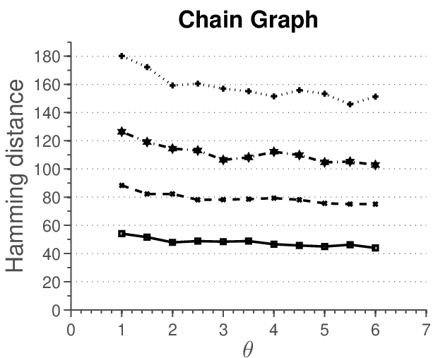
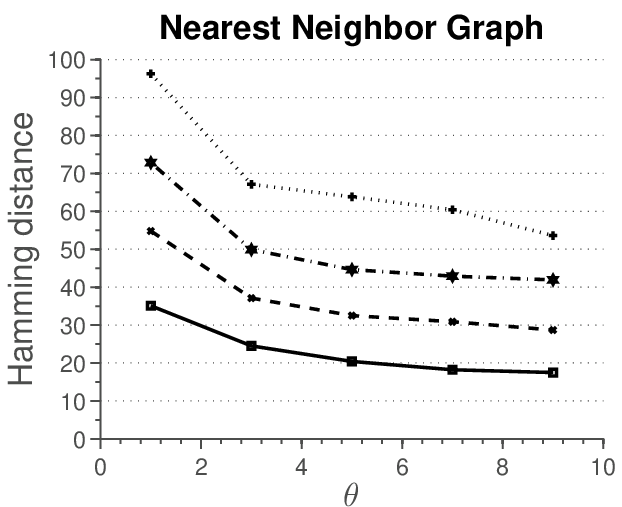
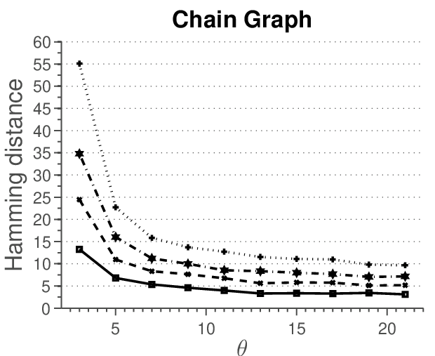
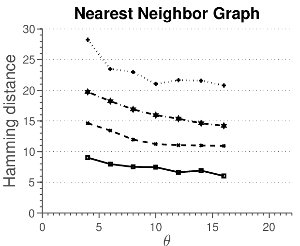
Theoretical results given in 3 characterize the sample size needed for consistent recovery of the underlying graph. In particular, Proposition 4 suggests that we need samples to estimate the graph structure consistently, for some . Therefore, if we plot the hamming distance between the true and recovered graph against , we expect the curves to reach zero distance for different problem sizes at a same point. We verify this on randomly generated chain and nearest-neighbors graphs.

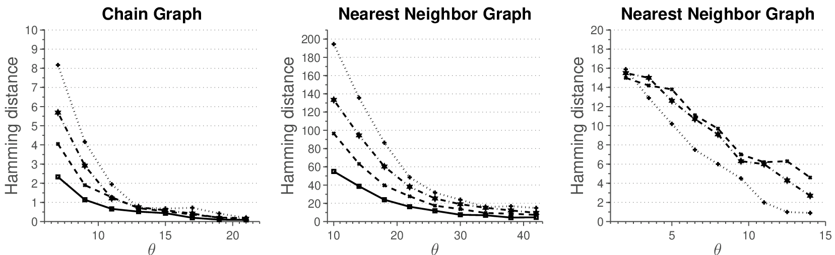

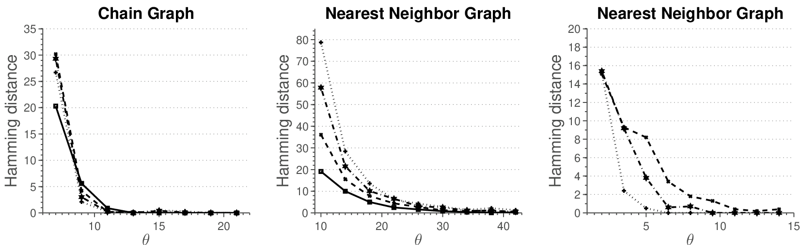
We generate data as follows. A random graph with nodes is created by first partitioning nodes into connected components, each with nodes, and then forming a random graph over these nodes. A chain graph is formed by permuting the nodes and connecting them in succession, while a nearest-neighbor graph is constructed following the procedure outlined in Li and Gui (2006). That is, for each node, we draw a point uniformly at random on a unit square and compute the pairwise distances between nodes. Each node is then connected to closest neighbors. Since some of nodes will have more than adjacent edges, we randomly remove edges from nodes that have degree larger than until the maximum degree of a node in a network is . Once the graph is created, we construct a precision matrix, with non-zero blocks corresponding to edges in the graph. Elements of diagonal blocks are set as , , while off-diagonal blocks have elements with the same value, for chain graphs and for nearest-neighbor networks. Finally, we add to the precision matrix, so that its minimum eigenvalue is equal to . Note that for the chain graph and for the nearest-neighbor graph. Simulation results are averaged over 100 replicates.
Figure 1 shows simulation results. Each row in the figure reports results for one method, while each column in the figure represents a different simulation setting. For the first two columns, we set and vary the total number of nodes in the graph. The third simulation setting sets the total number of nodes and changes the number of attributes . In the case of the chain graph, we observe that for small sample sizes the method of Danaher et al. (2011) outperforms all the other methods. We note that the multi-attribute method is estimating many more parameters, which require large sample size in order to achieve high accuracy. However, as the sample size increases, we observe that multi-attribute method starts to outperform the other methods. In particular, for the sample size indexed by all the graph are correctly recovered, while other methods fail to recover the graph consistently at the same sample size. In the case of nearest-neighbor graph, none of the methods recover the graph well for small sample sizes. However, for moderate sample sizes, multi-attribute method outperforms the other methods. Furthermore, as the sample size increases none of the other methods recover the graph exactly. This suggests that the conditions for consistent graph recovery may be weaker in the multi-attribute setting.








5.1 Alternative Structure of Off-diagonal Blocks
In this section, we investigate performance of different estimation procedures under different assumptions on the elements of the off-diagonal blocks of the precision matrix.
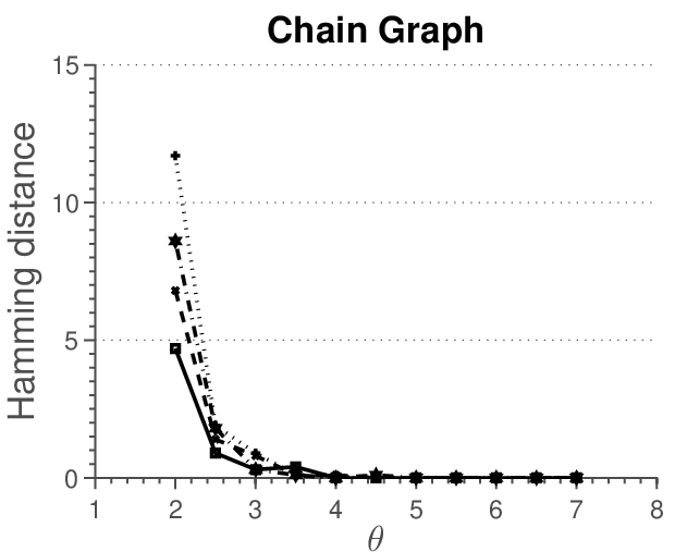
First, we investigate a situation where the multi-attribute method does not perform as well as the methods that estimate multiple graphical models. One such situation arises when different attributes are conditionally independent. To simulate this situation, we use the data generating approach as before, however, we make each block of the precision matrix a diagonal matrix. Figure 3 summarizes results of the simulation. We see that the methods of Danaher et al. (2011) and Guo et al. (2011) perform better, since they are estimating much fewer parameters than the multi-attribute method. does not utilize any structural information underlying the estimation problem and requires larger sample size to correctly estimate the graph than other methods.
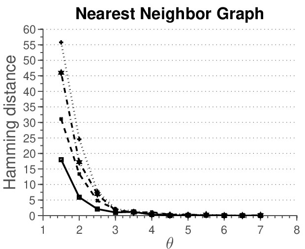
A completely different situation arises when the edges between nodes can be inferred only based on inter-attribute data, that is, when a graph based on any individual attribute is empty. To generate data under this situation, we follow the procedure as before, but with the diagonal elements of the off-diagonal blocks set to zero. Figure 5 summarizes results of the simulation. In this setting, we clearly see the advantage of the multi-attribute method, compared to other three methods. Furthermore, we can see that does better than multi-graph methods of Danaher et al. (2011) and Guo et al. (2011). The reason is that can identify edges based on inter-attribute relationships among nodes, while multi-graph methods rely only on intra-attribute relationships. This simulation illustrates an extreme scenario where inter-attribute relationships are important for identifying edges.
So far, off-diagonal blocks of the precision matrix were constructed to have constant values. Now, we use the same data generating procedure, but generate off-diagonal blocks of a precision matrix in a different way. Each element of the off-diagonal block is generated independently and uniformly from the set . The results of the simulation are given in Figure 7. Again, qualitatively, the results are similar to those given in Figure 1, except that in this setting more samples are needed to recover the graph correctly.
5.2 Different Number of Samples per Attribute
In this section, we show how to deal with a case when different number of samples is available per attribute. As noted in 2.2, we can treat non-measured attributes as missing completely at random (see Kolar and Xing, 2012, for more details).
Let be an indicator matrix, which denotes for each sample point the components that are observed. Then the sample covariance matrix is estimated as This estimate is plugged into the objective in (4).

We generate a chain graph with nodes, construct a precision matrix associated with the graph and attributes, and generate samples, . Next, we generate additional , and samples from the same model, but record only the values for the first attribute. Results of the simulation are given in Figure 8. Qualitatively, the results are similar to those presented in Figure 1.
6 Illustrative Applications to Real Data
In this section, we illustrate how to apply our method to data arising in studies of biological regulatory networks and Alzheimer’s disease.
6.1 Analysis of a Gene/Protein Regulatory Network
We provide illustrative, exploratory analysis of data from the well-known NCI-60 database, which contains different molecular profiles on a panel of 60 diverse human cancer cell lines. Data set consists of protein profiles (normalized reverse-phase lysate arrays for 92 antibodies) and gene profiles (normalized RNA microarray intensities from Human Genome U95 Affymetrix chip-set for genes). We focus our analysis on a subset of 91 genes/proteins for which both types of profiles are available. These profiles are available across the same set of cancer cells. More detailed description of the data set can be found in Katenka and Kolaczyk (2011).
We inferred three types of networks: a network based on protein measurements alone, a network based on gene expression profiles and a single gene/protein network. For protein and gene networks we use the glasso, while for the gene/protein network, we use our procedure outlined in 2.2. We use the stability selection (Meinshausen and Bühlmann, 2010) procedure to estimate stable networks. In particular, we first select the penalty parameter using cross-validation, which over-selects the number of edges in a network. Next, we use the selected to estimate 100 networks based on random subsamples containing 80% of the data-points. Final network is composed of stable edges that appear in at least 95 of the estimated networks. Table 1 provides a few summary statistics for the estimated networks. Furthermore, protein and gene/protein networks share edges, while gene and gene/protein networks share edges. Gene and protein network share only edges. Finally, edges are unique to gene/protein network. Figure 9 shows node degree distributions for the three networks. We observe that the estimated networks are much sparser than the association networks in Katenka and Kolaczyk (2011), as expected due to marginal correlations between a number of nodes. The differences in networks require a closer biological inspection by a domain scientist.
| protein network | gene network | gene/protein network | |
| Number of edges | 122 | 214 | 249 |
|---|---|---|---|
| Density | 0.03 | 0.05 | 0.06 |
| Largest connected component | 62 | 89 | 82 |
| Avg Node Degree | 2.68 | 4.70 | 5.47 |
| Avg Clustering Coefficient | 0.0008 | 0.001 | 0.003 |

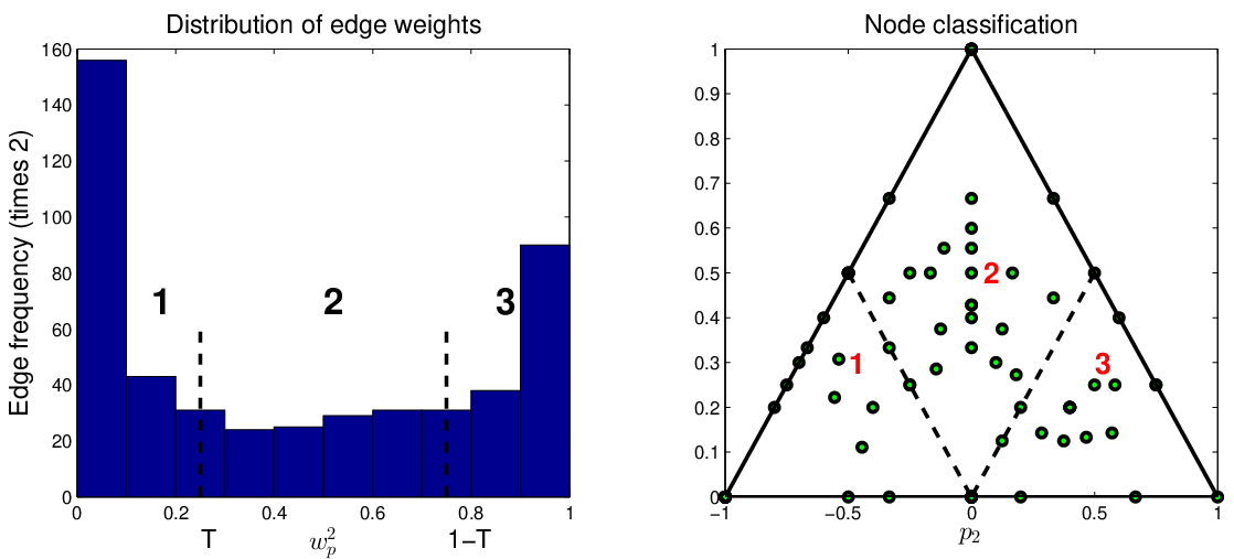
We proceed with a further exploratory analysis of the gene/protein network. We investigate the contribution of two nodal attributes to the existence of an edges between the nodes. Following Katenka and Kolaczyk (2011), we use a simple heuristic based on the weight vectors to classify the nodes and edges into three classes. For an edge between the nodes and , we take one weight vector, say , and normalize it to have unit norm. Denote the component corresponding to the protein attribute. Left plot in Figure 10 shows the values of over all edges. The edges can be classified into three classes based on the value of . Given a threshold , the edges for which are classified as gene-influenced, the edges for which are classified as protein influenced, while the remainder of the edges are classified as mixed type. In the left plot of Figure 10, the threshold is set as . Similar classification can be performed for nodes after computing the proportion of incident edges. Let , and denote proportions of gene, protein and mixed edges, respectively, incident with a node. These proportions are represented in a simplex in the right subplot of Figure 10. Nodes with mostly gene edges are located in the lower left corner, while the nodes with mostly protein edges are located in the lower right corner. Mixed nodes are located in the center and towards the top corner of the simplex. Further biological enrichment analysis is possible (see Katenka and Kolaczyk (2011)), however, we do not pursue this here.
6.2 Uncovering Functional Brain Network
We apply our method to the Positron Emission Tomography dataset, which contains 259 subjects, of whom 72 are healthy, 132 have mild cognitive Impairment and 55 are diagnosed as Alzheimer’s & Dementia. Note that mild cognitive impairment is a transition stage from normal aging to Alzheimer’s & Dementia. The data can be obtained from http://adni.loni.ucla.edu/. The preprocessing is done in the same way as in Huang et al. (2009).


Each Positron Emission Tomography image contains voxels. The effective brain region contains voxels, which are partitioned into regions, ignoring the regions with fewer than voxels. The largest region contains voxels and the smallest region contains voxels. Our preprocessing stage extracts representative voxels from these regions using the -median clustering algorithm. The parameter is chosen differently for each region, proportionally to the initial number of voxels in that region. More specifically, for each category of subjects we have an matrix, where is the number of subjects and is the number of voxels. Next we set , the number of representative voxels in region , . The representative voxels are identified by running the -median clustering algorithm on a sub-matrix of size with .
We inferred three networks, one for each subtype of subjects using the procedure outlined in 2.2. Note that for different nodes we have different number of attributes, which correspond to medians found by the clustering algorithm. We use the stability selection (Meinshausen and Bühlmann, 2010) approach to estimate stable networks. The stability selection procedure is combined with our estimation procedure as follows. We first select the penalty parameter in (4) using cross-validation, which overselects the number of edges in a network. Next, we create subsampled data sets, each of which contain of the data points, and estimate one network for each dataset using the selected . The final network is composed of stable edges that appear in at least of the estimated networks.
We visualize the estimated networks in Figure 11. Table 2 provides a few summary statistics for the estimated networks. Appendix D contains names of different regions, as well as the adjacency matrices for networks. From the summary statistics, we can observe that in normal subjects there are many more connections between different regions of the brain. Loss of connectivity in Alzheimer’s & Dementia has been widely reported in the literature (Greicius et al., 2004, Hedden et al., 2009, Andrews-Hanna et al., 2007, Wu et al., 2011).
Learning functional brain connectivity is potentially valuable for early identification of signs of Alzheimer’s disease. Huang et al. (2009) approach this problem using exploratory data analysis. The framework of Gaussian graphical models is used to explore functional brain connectivity. Here we point out that our approach can be used for the same exploratory task, without the need to reduce the information in the whole brain to one number. For example, from our estimates, we observe the loss of connectivity in the cerebellum region of patients with Alzheimer’s disease, which has been reported previously in Sjöbeck and Englund (2001). As another example, we note increased connectivity between the frontal lobe and other regions in the patients, which was linked to compensation for the lost connections in other regions (Stern, 2006, Gould et al., 2006).
| Healthy | Mild Cognitive | Alzheimer’s & | |
| subjects | Impairment | Dementia | |
| Number of edges | 116 | 84 | 59 |
| Density | 0.030 | 0.020 | 0.014 |
| Largest connected component | 48 | 27 | 25 |
| Avg Node Degree | 2.40 | 1.73 | 1.2 |
| Avg Clustering Coefficient | 0.001 | 0.0023 | 0.0007 |
Acknowledgments
We thank Eric D. Kolaczyk and Natallia V. Katenka for sharing preprocessed data used in their study with us. Eric P. Xing is partially supported through the grants NIH R01GM087694 and AFOSR FA9550010247. The research of Han Liu is supported by NSF grant IIS-1116730.
References
- Andrews-Hanna et al. (2007) J. R. Andrews-Hanna, A. Z. Snyder, J. L. Vincent, C. Lustig, D. Head, M. E. Raichle, and R.L. Buckner. Disruption of large-scale brain systems in advanced aging. Neuron, 56:924–935, 2007.
- Banerjee et al. (2008) O. Banerjee, L. El Ghaoui, and A. d’Aspremont. Model selection through sparse maximum likelihood estimation. J. Mach. Learn. Res., 9:485–516, 2008.
- Beck and Teboulle (2009) A. Beck and M. Teboulle. A fast iterative shrinkage-thresholding algorithm for linear inverse problems. SIAM J. Imag. Sci., 2:183–202, 2009.
- Cai et al. (2011) T. Cai, W. Liu, and X. Luo. A constrained minimization approach to sparse precision matrix estimation. J. Am. Statist. Assoc., 106:594–607, 2011.
- Chiquet et al. (2011) J. Chiquet, Y. Grandvalet, and C. Ambroise. Inferring multiple graphical structures. Stat. Comput., 21(4):537–553, 2011.
- Danaher et al. (2011) P. Danaher, P. Wang, and D. M. Witten. The joint graphical lasso for inverse covariance estimation across multiple classes. Technical report, University of Washington, 2011.
- Dempster (1972) Arthur P. Dempster. Covariance selection. Biometrics, 28:157–175, 1972.
- Friedman et al. (2008) J. H. Friedman, T. J. Hastie, and R. J. Tibshirani. Sparse inverse covariance estimation with the graphical lasso. Biostatistics, 9(3):432–441, 2008.
- Gould et al. (2006) R. L. Gould, B. Arroyo, R. G. Brown, A. M. Owen, E. T. Bullmore, and R. J. Howard. Brain mechanisms of successful compensation during learning in alzheimer disease. Neurology, 67(6):1011–1017, 2006.
- Greicius et al. (2004) M. D. Greicius, G. Srivastava, A. L. Reiss, and V. Menon. Default-mode network activity distinguishes alzheimer’s disease from healthy aging: evidence from functional mri. Proc. Natl. Acad. Sci. USA, 101(13):4637–4642, 2004.
- Guo et al. (2011) J. Guo, E. Levina, G. Michailidis, and J. Zhu. Joint estimation of multiple graphical models. Biometrika, 98(1):1–15, 2011.
- Hedden et al. (2009) T. Hedden, K. R. A. Van Dijk, J. A. Becker, A. Mehta, R. A. Sperling, K. A. Johnson, and R. L. Buckner. Disruption of functional connectivity in clinically normal older adults harboring amyloid burden. J. Neurosci., 29(40):12686–12694, 2009.
- Honorio and Samaras (2010) Jean Honorio and Dimitris Samaras. Multi-task learning of Gaussian graphical models. In Johannes Fürnkranz and Thorsten Joachims, editors, Proc. 27 Int. Conf. Mach. Learn., pages 447–454. Omnipress, Haifa, Israel, June 2010.
- Huang et al. (2009) Shuai Huang, Jing Li, Liang Sun, Jun Liu, Teresa Wu, Kewei Chen, Adam Fleisher, Eric Reiman, and Jieping Ye. Learning brain connectivity of alzheimer’s disease from neuroimaging data. In Y. Bengio, D. Schuurmans, J. Lafferty, C. K. I. Williams, and A. Culotta, editors, Adv. Neural Inf. Proc. Sys. 22, pages 808–816. 2009.
- Johnson et al. (2012) C. Johnson, A. Jalali, and P. Ravikumar. High-dimensional sparse inverse covariance estimation using greedy methods. In Neil Lawrence and Mark Girolami, editors, Proc. 15 Int. Conf. Artif. Intel. Statist., pages 574–582. 2012.
- Katenka and Kolaczyk (2011) Natallia Katenka and Eric D. Kolaczyk. Multi-attribute networks and the impact of partial information on inference and characterization. Ann. Appl. Stat., 6(3):1068–1094, 2011.
- Kolar and Xing (2012) Mladen Kolar and Eric P. Xing. Consistent covariance selection from data with missing values. In John Langford and Joelle Pineau, editors, Proc. 29 Int. Conf. Mach. Learn., pages 551–558, New York, NY, USA, July 2012. Omnipress. ISBN 978-1-4503-1285-1.
- Kolar et al. (2010) Mladen Kolar, Le Song, Amr Ahmed, and Eric P. Xing. Estimating Time-Varying networks. Ann. Appl. Statist., 4(1):94—123, 2010.
- Lam and Fan (2009) Clifford Lam and Jianqing Fan. Sparsistency and rates of convergence in large covariance matrix estimation. Ann. Statist., 37:4254–4278, 2009.
- Lauritzen (1996) S. L. Lauritzen. Graphical Models (Oxford Statistical Science Series). Oxford University Press, USA, July 1996.
- Li and Gui (2006) H. Li and J. Gui. Gradient directed regularization for sparse Gaussian concentration graphs, with applications to inference of genetic networks. Biostatistics, 7(2):302–317, 2006.
- Lounici et al. (2011) Karim Lounici, Massimiliano Pontil, Alexandre B Tsybakov, and Sara van de Geer. Oracle inequalities and optimal inference under group sparsity. Ann. Statist., 39:2164–204, 2011.
- Mazumder and Agarwal (2011) R. Mazumder and D. K. Agarwal. A flexible, scalable and efficient algorithmic framework for primal graphical lasso. Technical report, Stanford University, 2011.
- Mazumder and Hastie (2012) R. Mazumder and T. J. Hastie. Exact covariance thresholding into connected components for large-scale graphical lasso. J. Mach. Learn. Res., 13:781–794, 2012.
- Meinshausen and Bühlmann (2006) N. Meinshausen and P. Bühlmann. High dimensional graphs and variable selection with the lasso. Ann. Statist., 34(3):1436–1462, 2006.
- Meinshausen and Bühlmann (2010) N. Meinshausen and P. Bühlmann. Stability selection. J. R. Statist. Soc. B, 72(4):417–473, 2010.
- Peng et al. (2009) Jie Peng, Pei Wang, Nengfeng Zhou, and Ji Zhu. Partial correlation estimation by joint sparse regression models. J. Am. Statist. Assoc., 104(486):735–746, 2009.
- Rao (1969) B. Rao. Partial canonical correlations. Trabajos de Estadística y de Investigación Operativa, 20(2):211–219, 1969.
- Ravikumar et al. (2011) P. Ravikumar, M. J. Wainwright, G. Raskutti, and B. Yu. High-dimensional covariance estimation by minimizing -penalized log-determinant divergence. Electron. J. Statist., 5:935–980, 2011.
- Shen et al. (2012) X. Shen, W. Pan, and Y. Zhu. Likelihood-based selection and sharp parameter estimation. J. Am. Statist. Assoc., 107:223–232, 2012.
- Sjöbeck and Englund (2001) Martin Sjöbeck and Elisabet Englund. Alzheimer’s disease and the cerebellum: a morphologic study on neuronal and glial changes. Dementia and geriatric cognitive disorders, 12(3):211–218, 2001.
- Stern (2006) Yaakov Stern. Cognitive reserve and alzheimer disease. Alzheimer Disease & Associated Disorders, 20(2):112–117, 2006.
- Tseng (2001) P. Tseng. Convergence of a block coordinate descent method for nondifferentiable minimization. J. Optim. Theory Appl., 109(3):475–494, 2001.
- Varoquaux et al. (2010) Gael Varoquaux, Alexandre Gramfort, Jean-Baptiste Poline, and Bertrand Thirion. Brain covariance selection: better individual functional connectivity models using population prior. In J. Lafferty, C. K. I. Williams, J. Shawe-Taylor, R.S. Zemel, and A. Culotta, editors, Adv. Neural Inf. Proc. Sys. 23, pages 2334–2342. 2010.
- Witten et al. (2011) D. M. Witten, J. H. Friedman, and N. Simon. New insights and faster computations for the graphical lasso. J. Comput. Graph. Stat., 20(4):892–900, 2011.
- Wu et al. (2011) X. Wu, R. Li, A. S. Fleisher, E. M. Reiman, X. Guan, Y. Zhang, K. Chen, and L. Yao. Altered default mode network connectivity in alzheimer’s disease—a resting functional mri and bayesian network study. Human brain mapping, 32(11):1868–1881, 2011.
- Yuan (2010) Ming Yuan. High dimensional inverse covariance matrix estimation via linear programming. J. Mach. Learn. Res., 11:2261–2286, 2010.
- Yuan and Lin (2006) Ming Yuan and Yi Lin. Model selection and estimation in regression with grouped variables. J. R. Statist. Soc. B, 68:49–67, 2006.
- Yuan and Lin (2007) Ming Yuan and Yi Lin. Model selection and estimation in the gaussian graphical model. Biometrika, 94(1):19–35, 2007.
- Zhao et al. (2012) T. Zhao, H. Liu, K. E. Roeder, J. D. Lafferty, and L. A. Wasserman. The huge package for high-dimensional undirected graph estimation in r. J. Mach. Learn. Res., 13:1059–1062, 2012.
Appendix A Efficient Updates of the Precision and Covariance Matrices
Our algorithm consists of updating the precision matrix by solving optimization problems (7) and (8) and then updating the estimate of the covariance matrix. Both steps can be performed efficiently.
The estimate of the covariance matrix can be updated efficiently, without inverting the whole matrix, using the matrix inversion lemma as follows
| (13) | ||||
with .
Appendix B Complexity Analysis of Multi-attribute Estimation
Step 2 of the estimation algorithm updates portions of the precision and covariance matrices corresponding to one node at a time. From A, we observe that the computational complexity of updating the precision matrix is . Updating the covariance matrix requires computing , which can be efficiently done in operations, assuming that . With this, the covariance matrix can be updated in operations. Therefore the total cost of updating the covariance and precision matrices is operations. Since step 2 needs to be performed for each node , the total complexity is . Let denote the total number of times step 2 is executed. This leads to the overall complexity of the algorithm as . In practice, we observe that for sparse graphs. Furthermore, when the whole solution path is computed, we can use warm starts to further speed up computation, leading to for each .
Appendix C Technical Proofs
In this appendix, we collect proofs of the results presented in the main part of the paper.
C.1 Proof of Lemma 1
We start the proof by giving to technical results needed later. The following lemma states that the minimizer of (4) is unique and has bounded minimum and maximum eigenvalues, denoted as and .
Lemma 5.
For every value of , the optimization problem in Eq. (4) has a unique minimizer , which satisfies and .
Proof.
The optimization objective given in (4) can be written in the equivalent constrained form as
The procedure involves minimizing a continuous objective over a compact set, and so by Weierstrass’ theorem, the minimum is always achieved. Furthermore, the objective is strongly convex and therefore the minimum is unique.
The solution to the optimization problem (4) satisfies
| (14) |
where is the element of the sub-differential and satisfies for all . Therefore,
Next, we prove an upper bound on . At optimum, the primal-dual gap is zero, which gives that
as and . Since , the proof is done. ∎
The next results states that the objective function has a Lipschitz continuous gradient, which will be used to show that the generalized gradient descent can be used to find .
Lemma 6.
The function has a Lipschitz continuous gradient on the set , with the Lipschitz constant .
Proof.
We have that . Then
which completes the proof. ∎
Now, we provide the proof of Lemma 1.
By construction, the sequence of estimates decrease the objective value and are positive definite.
To prove the convergence, we first introduce some additional notation. Let and . For any , let
be a quadratic approximation of at a given point , which has a unique minimizer
From Lemma 2.3. in Beck and Teboulle (2009), we have that
| (15) |
if . Note that always holds if is as large as the Lipschitz constant of .
Let and denote two successive iterates obtained by the procedure. Without loss of generality, we can assume that is obtained by updating the rows/columns corresponding to the node . From (15), it follows that
| (16) |
where is a current estimate of the Lipschitz constant. Recall that in our procedure the scalar serves as a local approximation of . Since eigenvalues of are bounded according to Lemma 5, we can conclude that the eigenvalues of are bounded as well. Therefore the current Lipschitz constant is bounded away from zero, using Lemma 6. Combining the results, we observe that the right hand side of (16) converges to zero as , since the optimization procedure produces iterates that decrease the objective value. This shows that converges to zero, for any . Since is a bounded sequence, it has a limit point, which we denote . It is easy to see, from the stationary conditions for the optimization problem given in (6), that the limit point also satisfies the global KKT conditions to the optimization problem in (4).
C.2 Proof of Lemma 3
Suppose that the solution to (4) is block diagonal with blocks . For two nodes in different blocks, we have that as the inverse of the block diagonal matrix is block diagonal. From the KKT conditions, it follows that .
Now suppose that for all . For every construct
Then is the solution of (4) as it satisfies the KKT conditions.
C.3 Proof of Eq. (3)
First, we note that
is the conditional covariance matrix of given the remaining nodes (see Proposition C.5 in Lauritzen (1996)). Define . Partial canonical correlation between and is equal to zero if and only if . On the other hand, the matrix inversion lemma gives that . Now, if and only if . This shows the equivalence relationship in Eq. (3).
C.4 Proof of Proposition 4
We provide sufficient conditions for consistent network estimation. Proposition 4 given in 3 is then a simple consequence. To provide sufficient conditions, we extend the work of Ravikumar et al. (2011) to our setting, where we observe multiple attributes for each node. In particular, we extend their Theorem 1.
For simplicity of presentation, we assume that , for all , that is, we assume that the same number of attributes is observed for each node. Our assumptions involve the Hessian of the function evaluated at the true ,
| (17) |
and the true covariance matrix . The Hessian and the covariance matrix can be thought of block matrices with blocks of size and , respectively. We will make use of the operator that operates on these block matrices and outputs a smaller matrix with elements that equal to the Frobenius norm of the original blocks,
In particular, and .
We denote the index set of the non-zero blocks of the precision matrix as
and let denote its complement in , that is,
As mentioned earlier, we need to make an assumption on the Hessian matrix, which takes the standard irrepresentable-like form. There exists a constant such that
| (18) |
These condition extends the irrepresentable condition given in Ravikumar et al. (2011), which was needed for estimation of networks from single attribute observations. It is worth noting, that the condition given in Eq. (18) can be much weaker than the irrepresentable condition of Ravikumar et al. (2011) applied directly to the full Hessian matrix. This can be observed in simulations done in 5, where a chain network is not consistently estimated even with a large number of samples.
We will also need the following two quantities to specify the results
| (19) |
and
| (20) |
Finally, the results are going to depend on the tail bounds for the elements of the matrix . We will assume that there is a constant and a function such that for any
| (21) |
The function will be monotonically increasing in both and . Therefore, we define the following two inverse functions
| (22) |
and
| (23) |
for .
With the notation introduced, we have the following result.
Theorem 7.
Theorem 7 is of the same form as Theorem 1 in Ravikumar et al. (2011), but the element-wise convergence is established for , which will guarantee successful recovery of non-zero partial canonical correlations if the blocks of the true precision matrix are sufficiently large.
Theorem 7 is proven as Theorem 1 in Ravikumar et al. (2011). We provide technical results in Lemma 8, Lemma 9 and Lemma 10, which can be used to substitute results of Lemma 4, Lemma 5 and Lemma 6 in Ravikumar et al. (2011) under our setting. The rest of the arguments then go through. Below we provide some more details.
First, let be the mapping defined as
| (26) |
Next, define the function
| (27) |
and the following system of equations
| (28) |
It is known that is the minimizer of optimization problem in Eq. (4) if and only if it satisfies the system of equations given in Eq. (28). We have already shown in Lemma 5 that the minimizer is unique.
Let be the solution to the following constrained optimization problem
| (29) |
Observe that one cannot find in practice, as it depends on the unknown set . However, it is a useful construction in the proof. We will prove that is solution to the optimization problem given in Eq. (4), that is, we will show that satisfies the system of equations (28).
Using the first-order Taylor expansion we have that
| (30) |
where and denotes the remainder term. With this, we state and prove Lemma 8, Lemma 9 and Lemma 10. They can be combined as in Ravikumar et al. (2011) to complete the proof of Theorem 7.
Lemma 8.
Proof.
Lemma 9.
Assume that
| (34) |
Then
| (35) |
Proof.
Lemma 10.
Assume that
| (36) |
Then
| (37) |
Proof.
The proof follows the proof of Lemma 6 in Ravikumar et al. (2011). Define the ball
the gradient mapping
and
We need to show that , which implies that .
Under the assumptions of the lemma, for any , we have the following decomposition
Using Lemma 9, the first term can be bounded as
where the last inequality follows under the assumptions. Similarly
This shows that . ∎
The following result is a corollary of Theorem 7, which shows that the graph structure can be estimated consistently under some assumptions.
Corollary 11.
Assume that the conditions of Theorem 7 are satisfied. Furthermore, suppose that
then Algorithm 1 estimates a graph which satisfies
Next, we specialize the result of Theorem 7 to a case where has sub-Gaussian tails. That is, the random vector is zero-mean with covariance . Each is sub-Gaussian with parameter .
Proposition 12.
The proof simply follows by observing that, for any ,
| (38) | ||||
for all with . Therefore,
Theorem 7 and some simple algebra complete the proof.
C.5 Some Results on Norms of Block Matrices
Let be a partition of . Throughout this section, we assume that matrices and a vector are partitioned into blocks according to .
Lemma 13.
| (39) |
Proof.
For any ,
∎
Lemma 14.
| (40) |
Proof.
Let and let be a partition of .
∎
Lemma 15.
| (41) |
Proof.
For a fixed and ,
Maximizing over and gives the result. ∎
Appendix D Additional Information About Functional Brain Networks
Table 3 contains list of the names of the brain regions. The number before each region is used to index the node in the connectivity models. Figures 12, 13 and 14 contain adjacency matrices for the estimated graph structures.


Precentral_L |
Fusiform_L | ||
Precentral_R |
Fusiform_R | ||
Frontal_Sup_L |
Postcentral_L | ||
Frontal_Sup_R |
Postcentral_R | ||
Frontal_Sup_Orb_L |
Parietal_Sup_L | ||
Frontal_Sup_Orb_R |
Parietal_Sup_R | ||
Frontal_Mid_L |
Parietal_Inf_L | ||
Frontal_Mid_R |
Parietal_Inf_R | ||
Frontal_Mid_Orb_L |
SupraMarginal_L | ||
Frontal_Mid_Orb_R |
SupraMarginal_R | ||
Frontal_Inf_Oper_L |
Angular_L | ||
Frontal_Inf_Oper_R |
Angular_R | ||
Frontal_Inf_Tri_L |
Precuneus_L | ||
Frontal_Inf_Tri_R |
Precuneus_R | ||
Frontal_Inf_Orb_L |
Paracentral_Lobule_L | ||
Frontal_Inf_Orb_R |
Paracentral_Lobule_R | ||
Rolandic_Oper_L |
Caudate_L | ||
Rolandic_Oper_R |
Caudate_R | ||
Supp_Motor_Area_L |
Putamen_L | ||
Supp_Motor_Area_R |
Putamen_R | ||
Frontal_Sup_Medial_L |
Thalamus_L | ||
Frontal_Sup_Medial_R |
Thalamus_R | ||
Frontal_Med_Orb_L |
Temporal_Sup_L | ||
Frontal_Med_Orb_R |
Temporal_Sup_R | ||
Rectus_L |
Temporal_Pole_Sup_L | ||
Rectus_R |
Temporal_Pole_Sup_R | ||
Insula_L |
Temporal_Mid_L | ||
Insula_R |
Temporal_Mid_R | ||
Cingulum_Ant_L |
Temporal_Pole_Mid_L | ||
Cingulum_Ant_R |
Temporal_Pole_Mid_R | ||
Cingulum_Mid_L |
Temporal_Inf_L | ||
Cingulum_Mid_R |
Temporal_Inf_R | ||
Hippocampus_L |
Cerebelum_Crus1_L | ||
Hippocampus_R |
Cerebelum_Crus1_R | ||
ParaHippocampal_L |
Cerebelum_Crus2_L | ||
ParaHippocampal_R |
Cerebelum_Crus2_R | ||
Calcarine_L |
Cerebelum_4_5_L | ||
Calcarine_R |
Cerebelum_4_5_R | ||
Cuneus_L |
Cerebelum_6_L | ||
Cuneus_R |
Cerebelum_6_R | ||
Lingual_L |
Cerebelum_7b_L | ||
Lingual_R |
Cerebelum_7b_R | ||
Occipital_Sup_L |
Cerebelum_8_L | ||
Occipital_Sup_R |
Cerebelum_8_R | ||
Occipital_Mid_L |
Cerebelum_9_L | ||
Occipital_Mid_R |
Cerebelum_9_R | ||
Occipital_Inf_L |
Vermis_4_5 | ||
Occipital_Inf_R |