Padé approximants and for the muon
Abstract:
The leading hadronic contribution to the muon anomalous magnetic moment is given by a weighted euclidean momentum integral of the hadronic vacuum polarization. This integral is dominated by momenta of order the muon mass. Since in lattice QCD it is difficult to compute the vacuum polarization at a large number of low momenta, a parametrization of the vacuum polarization is required to extrapolate the data. Most fits to date are based on vector meson dominance, which introduces model dependence into the lattice computation of the magnetic moment. Here we introduce a model-independent extrapolation method, and present a few first tests of this new method.
June 24-29, 2012
Cairns, Australia
1 Introduction
The anomalous magnetic moment of the muon has been measured with great accuracy [1], and will be measured with even greater accuracy in the near future. Therefore, a reliable computation of from theory with a comparable error would provide a precision test of the Standard Model that is sensitive to a large class of models of new physics beyond the Standard Model. For this reason there has recently been a lot of interest in lattice computations of with controlled errors [2, 3, 4, 5]; for an overview, and more references, we refer to Ref. [6]. Here, we report on recent work on the leading hadronic contribution to , which comes from the hadronic vacuum polarization [7].
The contribution to from the lowest-order hadronic vacuum polarization can be written as an integral over the subtracted vacuum polarization as a function of euclidean [8, 9],
| (1) |
where is a kinematic weight shown in Fig. 1, left panel. The right panel shows a typical example of lattice data for (these are the data from a lattice with lattice spacing fm and MeV discussed below).

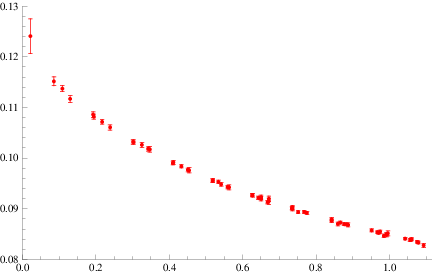
Clearly, one needs to fit these data in order to compute the integral. In most lattice computations of to date this has been done with various variants of vector-meson dominance (VMD).11 1 Ref. [5] used Padé approximants, but, as we will see below, of a different type than those supported by a convergence theorem. This introduces model dependence into the computation, and the aim of the work presented here is to remove this model dependence.
2 Multi-point Padé approximants
We start from the observation that we can write a subtracted dispersion relation for :
| (2) |
in which is the spectral function. Because the spectral function , the integral in Eq. (2) is a Stieltjes function, analytic everywhere except along the cut .
Theorem:
Given points , ,
a sequence of Padé approximants
(PAs) can be constructed which converge to on any closed,
bounded region of the complex plane excluding the cut, in the limit .
This sequence of PAs can be constructed from the points through a continued fraction:
| (3) |
with related to (, etc.). Equation (3) yields a PA (where is the integer part of ). Furthermore, one can prove that this can be rewritten as [10, 11, 12]
| (4) |
with
| (5) |
i.e., all poles are single poles, they are located on the cut, and all residues are positive. The constant for even.
In the situation of an actual fit to data for obtained from a numerical computation, these data are only known within some statistical errors. That implies that we do not know any points of the function exactly, and a multi-point sequence of PAs as implied by the theorem cannot be constructed. Our strategy will be to fit a fixed number of data points on a given interval, using the fact that since , according to the theorem, can be described by a converging sequence of PAs of the form (4), this equation provides a valid functional form to which to fit the data. More concretely, we will fit the form (4) for ; this yields , , and PAs. In order to compare diffferent fits, we will then compute
| (6) |
We note that VMD is the same as a PA, but keeping fixed: This is not a valid PA in the sense of the theorem, because the theorem does not say anything about the possible values of the parameters in addition to the conditions (5).
3 Tests
For our first test, we explore fits to a MILC data set on a lattice with lattice spacing fm, and a pion mass MeV [13]. This is one of the data sets that was also used in Ref. [2]. We show the results for the PAs and for VMD in Table 1. The uncorrelated VMD fit is the same as the fit to these data performed in Ref. [2], and the results agree.
| correlated | uncorrelated | ||||
|---|---|---|---|---|---|
| interval GeV2 | interval GeV2 | ||||
| PA | # parameters | /dof | /dof | ||
| VMD | 2 | 5.86/3∗ | 363(7) | 4.37/18 | 413(8) |
| 3 | 11.4/8 | 338(6) | 3.58/17 | 373(37) | |
| 4 | 7.49/7 | 350(8) | 3.36/16 | 424(116) | |
| 5 | 7.49/6 | 350(8) | 3.35/15 | 443(293) | |
| 6 | 7.49/5 | 350(7) | 3.35/14 | 445(432) | |
Table 1 leads us to make the following observations:
- •
The correlated VMD fit is a bad fit as measured by per degree of freedom (dof); adding parameters the fits clearly improve. Note that we always choose the fitting interval by looking for a minimal value of /dof.
- •
It turns out that it is difficult to determine the parameters of the second pole with any precision [7] (as can be inferred from the values of /dof), but is insensitive to the second and higher poles.
- •
There is good internal consistency between all fits shown in the table, except between the uncorrelated VMD fit and any of the correlated PA fits. However, the VMD fits are model dependent, which translates into an unknown systematic error in these fits.


We display some of the fits of Table 1 in Fig. 2. Not surprisingly, the uncorrelated fits look better at small , but all fits shown in the figure do a good job of describing the data. Therefore, based on the data, it is not possible to decide which of these fits is the best fit.
We repeated our explorative analysis on MILC lattices on a lattice with lattice spacing fm, and MeV. We find very similar results;22 2 Of course, central values of are quite different, if only because of the smaller pion mass. in particular we find
| (7) | |||||
Our conclusions are the same as before. We note that for both data sets the discrepancy between the correlated PA and the uncorrelated VMD fit is about 15%. From the point of view that both types of fit give a good description of the data, we take this to imply that there is a systematic error of (at least) this size afflicting the determination of from the lattice.

The underlying problem is displayed in Fig. 3, where we see that there are essentially no data in the region dominating the integral in Eq. (1). For this, one clearly needs data at more low values of , with smaller errors. It would be interesting to see whether these improvements can be attained by using twisted boundary conditions, something that has been tried in this context in Ref. [5], and by an error reduction technique such as that proposed in Ref. [14].
We have also compared our PA fits with polynomial fits; results are shown in Table 2. “Poly ” indicates a fit with a polynomial of degree . All fits are correlated fits; and the pairs of fits “Poly 3,” “” respectively “Poly 4,” “” have the same number of parameters. We observe that the fits deteriorate in the polynomial case going from Poly 3 to Poly 4, with errors increasing, and central values for fluctuating more, while this is not the case going from the to the PA fit.
| Poly 3 | Poly 4 | PA [1,1] | PA [1,2] | |||||
|---|---|---|---|---|---|---|---|---|
| # points | /dof | /dof | /dof | /dof | ||||
| 16 | 9.6/12 | 543(35) | 9.5/11 | 483(244) | 9.7/12 | 564(55) | 9.7/11 | 565(41) |
| 18 | 11.4/14 | 526(33) | 10.5/13 | 596(79) | 11.2/14 | 541(46) | 11.5/13 | 561(21) |
| 20 | 13.1/16 | 536(23) | 13.1/15 | 535(45) | 13.9/16 | 572(41) | 13.9/15 | 572(37) |
| 22 | 16.5/18 | 541(23) | 15.9/17 | 513(44) | 18.5/18 | 566(37) | 18.5/17 | 566(33) |
| 24 | 16.6/20 | 537(18) | 16.4/19 | 521(41) | 19.4/20 | 583(34) | 19.4/19 | 583(33) |
| 26 | 30.7/22 | 505(16) | 23.6/21 | 580(32) | 26.8/22 | 557(31) | 26.7/21 | 560(27) |
4 Conclusions
We presented a new method for parametrizing the momentum dependence of the hadronic vacuum polarization, with the aim to avoid the model dependence of the VMD-based fits that up to this point have been used in most fits to lattice data for the hadronic vacuum polarization. It turns out that this is possible, because the vacuum polarization can be represented in terms of a Stieltjes function, for which sequences of Padé approximants can be constructed which converge uniformly to the function on any bounded region in the complex place excluding the cut.
We have tested this new idea on two examples of lattice data for the vacuum polarization. We note that the fits based on Padé approximants can lead to larger statistical errors than some of the VMD fits, as for instance in Eq. (7). However, it should be emphasized that the latter are afflicted with an unknown systematic error originating in the inherent model dependence of VMD-based fits. The fits based on Padé approximants avoid this systematic error.33 3 Of course, there are other systematic errors, such as scaling violations, finite-size effects, and chiral extrapolation errors.
The new method looks promising. However, it is clear that data for the hadronic vacuum polarization at more low values (of order the square of the muon mass), and with smaller errors, will be needed in order to reach a higher precision for . As we have seen, fits based on Padé approximants and VMD-based fits (both correlated and uncorrelated) give a good description of the data, but lead to values for which differ by about 15%.
Finally, we observe that is an example of a quantity which is quite sensitive to the value of the pion mass. Therefore, better data for the hadronic vacuum polarization will also have to be obtained at small values of the pion mass, certainly significantly smaller than MeV.
Acknowledgements We would like to thank USQCD for the computing resources used to generate the vacuum polarization as well as the MILC collaboration for providing the configurations used. TB and MG are supported in part by the US Department of Energy under Grant No. DE-FG02-92ER40716 and Grant No. DE-FG03-92ER40711. MG is also supported in part by the Spanish Ministerio de Educación, Cultura y Deporte, under program SAB2011-0074. SP is supported by CICYTFEDER-FPA2008-01430, FPA2011-25948, SGR2009-894, the Spanish Consolider-Ingenio 2010 Program CPAN (CSD2007-00042) and also by the Programa de Movilidad PR2010-0284.
References
- [1] G. W. Bennett et al. [Muon Collaboration], Phys. Rev. D 73, 072003 (2006) [hep-ex/0602035]; Phys. Rev. Lett. 92, 161802 (2004) [hep-ex/0401008].
- [2] C. Aubin and T. Blum, Phys. Rev. D 75, 114502 (2007) [arXiv:hep-lat/0608011].
- [3] X. Feng, K. Jansen, M. Petschlies and D. B. Renner, Phys. Rev. Lett. 107, 081802 (2011) [arXiv:1103.4818 [hep-lat]].
- [4] P. Boyle, L. Del Debbio, E. Kerrane and J. Zanotti, arXiv:1107.1497 [hep-lat].
- [5] M. Della Morte, B. Jäger, A. Jüttner and H. Wittig, JHEP 1203, 055 (2012) [arXiv:1112.2894 [hep-lat]].
- [6] T. Blum, these proceedings.
- [7] C. Aubin, T. Blum, M. Golterman and S. Peris, Phys. Rev. D 86, 054509 (2012) [arXiv:1205.3695 [hep-lat]].
- [8] B. E. Lautrup, A. Peterman and E. De Rafael, Nuovo Cim. A 1, 238 (1971).
- [9] T. Blum, Phys. Rev. Lett. 91, 052001 (2003) [hep-lat/0212018].
- [10] G.A. Baker, Jr., J. Math. Phys. 10 814 (1969).
- [11] M. Barnsley, J. Math. Phys. 14 299 (1973).
- [12] G.A. Baker, P. Graves-Morris, Padé Approximants, 2nd ed. (Cambridge, 1996).
- [13] MILC collaboration, http://physics.indiana.edu/sg/milc.html .
- [14] T. Blum, T. Izubuchi and E. Shintani, arXiv:1208.4349 [hep-lat].