跳到论文正文
W Papers独立论文阅读器 arXiv:1210.7453 论文正文 计算阅读时间 · 0%
引用这篇论文根据当前论文元数据生成,正式投稿前建议核对。


License: arXiv.org perpetual non-exclusive license
arXiv:1210.7453v2 [hep-ph] 08 Apr 2013

Two-loop supersymmetric QCD corrections to Higgs-quark-quark couplings in the generic MSSM

Andreas Crivellin Email: crivellin@itp.unibe.ch Affiliation: Albert Einstein Center for Fundamental Physics, Institute for Theoretical Physics,
University of Bern, CH-3012 Bern, Switzerland.
   Christoph Greub Email: greub@itp.unibe.ch Affiliation: Albert Einstein Center for Fundamental Physics, Institute for Theoretical Physics,
University of Bern, CH-3012 Bern, Switzerland.
August 24, 2026
Abstract

In this article we compute the two-loop supersymmetric QCD corrections to Higgs-quark-quark couplings in the generic MSSM generated by diagrams involving squarks and gluinos. We give analytic results for the two-loop contributions in the limit of vanishing external momenta for general SUSY masses valid in the MSSM with general flavor structure.

Working in the decoupling limit (MSUSY≫vM_{\rm{SUSY}}\gg v) we resum all chirally enhanced corrections (related to Higgs-quark-quark couplings) up to order αs(n+1)​tann⁡β\alpha_{s}^{(n+1)}\tan^{n}\beta. This resummation allows for a more precise determination of the Yukawa coupling and CKM elements of the MSSM superpotential necessary for the study of Yukawa coupling unification.

The knowledge of the Yukawa couplings of the MSSM superpotential in addition allows us to derive the effective Higgs-quark-quark couplings entering FCNC processes. These effective vertices can in addition be used for the calculation of Higgs decays into quarks as long as MSUSY>MHiggsM_{\rm SUSY}>M_{\rm Higgs} holds. Furthermore, our calculation is also necessary for consistently including the chirally enhanced self-energy contributions into the calculation of FCNC processes in the MSSM beyond leading order.

At two-loop order, we find an enhancement of the SUSY threshold corrections, induced by the quark self-energies, of approximately 9%9\% for μ=MSUSY\mu=M_{\rm{SUSY}} compared to the one-loop result. At the same time, the matching scale dependence of the effective Higgs-quark-quark couplings is significantly reduced.

pacs
11.30.Pb,12.15.Ff,12.60.Jv,14.80.Da

I Introduction

In the MSSM diagrams with sfermions and gauginos as virtual particles generate important loop corrections to Higgs-quark-quark couplings. After the spontaneous breaking of S​U​(2)L⊗U​(1)YSU(2)_{L}\otimes U(1)_{Y} at the electroweak scale, the Higgs fields acquire their vacuum expectation values (VEVx),and the genuine vertex corrections to Higgs-quark-quark couplings also generate chirality changing quark self-energies (or self-masses). Thus, there is a one to one correspondence between loop corrections to three-point Higgs-quark-quark functions and quark self-energies: The correction to a Higgs-quark-quark coupling is given by the corresponding chirality-changing self-energy divided by the VEV of the involved Higgs field.

This means that we can simplify the calculation of three-point functions by reducing the problem to the calculation of two-point functions (self-energies). In this way, the self-energy contributions to quark masses can be directly related to effective Higgs-quark-quark couplings which allow for an efficient calculation of the effective Higgs vertices.

The quark self-energies also modify the relation between the Yukawa couplings of the MSSM superpotential and the quark masses (extracted from low-energy observables). Especially if tan⁡β\tan\beta (the ratio of the VEVs of the two Higgs fields) is large, these contributions are generically very large and can be of order one [1, 2, 3, 4]. In an analogous way, also the relation between the CKM matrix of the superpotential and the physical one is altered (by chargino-squark diagrams in the MSSM with MFV [8, 5, 9, 6, 7] and in addition by squark-gluino diagrams in the general MSSM [10, 11]). Because of these corrections the physical quark masses and the measured CKM elements no longer equal the ones that appear in the MSSM superpotential. One says that these relations are modified by so-called threshold corrections, i.e.. by the decoupling of heavy particles. Since in Higgs decays Higgs mediated FCNCs (like Bs⁡(d)B_{s(d)} mixing and Bs⁡(d)→μ+​μ−B_{s(d)}\to\mu^{+}\mu^{-}) and in Higgsino vertices the Yukawa couplings (of the superpotential) and not the physical quark masses enter, a precise knowledge of these quantities and thus of the threshold corrections is necessary. Furthermore, in GUT models with Yukawa coupling unification not the effective Yukawa coupling of the SM, but rather the Yukawas of the superpotential unify and the SUSY threshold corrections must be taken into account in order to judge whether they actually do unify [12, 13]. In conclusion, it is desirable to know the relation between the parameters of the MSSM superpotential and the physical, i.e.,measurable quantities, very precisely.

Having the relation between the Yukawa couplings (CKM elements) of the superpotential and the physical quark masses (physical CKM elements) at hand, one can calculate the effective Higgs couplings entering FCNC processes that include the SUSY loop corrections. This is most easily achieved by matching the MSSM on the two-Higgs-doublet model of type three (2HDM III). The loop-induced couplings of quarks to the “wrong” Higgs field, i.e., to the Higgs that is not involved in the Yukawa term in the superpotential, induce flavor-changing neutral Higgs couplings after switching to the physical basis in which the quark mass matrices are diagonal in flavor space. These effective Higgs couplings can be expressed entirely in terms of the physical masses and self-energies depending on MSSM parameters. Here a complication arises because these self-energies must be calculated using the Yukawa couplings and the CKM elements of the superpotential, which must have been determined previously in the process of renormalization by including the loop corrections, i.e., by resumming the threshold corrections. This problem can be solved analytically in the decoupling limit of the generic MSSM in which the self-energies are at most linear in the Yukawa couplings [14].

The importance of these threshold corrections and thus of the chirally enhanced self-energies motivates their calculation at NLO in αs\alpha_{s}. In the MSSM with MFV these corrections have been calculated in Refs. [15, 16], [17] and [18, 19]. Here we want to extend this analysis to the MSSM with generic sources of flavor violation and resum all chirally enhanced effects using the results of Refs. [10, 7, 20, 14]. In addition, working in the approximation of vanishing external momenta, we are able to give relatively simple analytic expressions for the self-energies, and therefore also the resummation of all chirally enhanced corrections can be (and is) performed analytically.

After discussing the quark self-energies (and their connection to Higgs-quark-quark couplings in the decoupling limit of the MSSM) in the next section, we derive the relations between the MSSM Yukawa couplings and the quark masses at LO in Sec. III. As the main result of this article we calculate the SQCD contribution to the chirality-changing self-energy at the two-loop level in Sec. IV. In Sec. V we discuss the topics of Sec. III at NLO. In Sec. VI we derive the effective Higgs-quark-quark couplings and conclude in Sec. VII. Various appendices summarize the relevant one-loop results.

II Quark self-energies, effective Lagrangian and the decoupling limit

As described in the Introduction, there is a one to one correspondence between chirality changing self-energies and Higgs-quark-quark couplings: In the decoupling limit of the MSSM (MSUSY>vM_{\rm{SUSY}}>v and MSUSY>pM_{\rm{SUSY}}>p, where pp is the external momentum) chirality changing self-energies are proportional to one power of a VEV only, and the corrections to the Higgs-quark-quark couplings can be obtained by dividing the corresponding self-energy by the VEV of the Higgs field involved. Thus, as long as the momentum flowing through the Higgs is small compared to the SUSY masses and the SUSY masses are heavier than the electroweak VEV, the decoupling limit is a valid approximation. In this approximation the calculation of the Higgs-quark-quark three-point function can be reduced to the calculation of quark self-energies. For this reason we will consider the quark self-energies in this section in some detail and discuss the decoupling limit. The analysis is valid independent of the loop order (concerning αs\alpha_{s} corrections) at which the self-energies are calculated.

In general, it is possible to decompose any quark (or any fermion) self-energy into chirality-flipping and chirality-conserving parts in the following way:

Σf​iq​(p)=(Σf​iq​L​R​(p2)+p/Σf​iq​R​R​(p2))​PR+(Σf​iq​R​L​(p2)+p/Σf​iq​L​L​(p2))​PL.\Sigma_{fi}^{q}(p)=\left({\Sigma_{fi}^{q\,LR}(p^{2})+p\hskip-4.40002pt/\hskip 0.59998pt\Sigma_{fi}^{q\,RR}(p^{2})}\right)P_{R}+\left({\Sigma_{fi}^{q\,RL}(p^{2})+p\hskip-4.40002pt/\hskip 0.59998pt\Sigma_{fi}^{q\,LL}(p^{2})}\right)P_{L}\,. (1)

Note that the chirality-flipping parts Σf​iq​R​L,L​R\Sigma_{fi}^{q\,RL,LR} have dimension mass, while the chirality conserving parts Σf​iq​L​L,R​R\Sigma_{fi}^{q\,LL,RR} are dimensionless.

In the following we will be interested in the contributions to Eq. (1) that involve heavy SUSY particles. The reason for this is that only these contributions lead to the threshold corrections entering the relation between the quark masses and the Yukawa couplings of the MSSM superpotential. It is convenient to work in an effective field theory in which the part of the effective Lagrangian containing mass terms and kinetic terms for the quarks is given by

ℒeffq¯​q=−(vqYqi⋆treeδf​i+Cq​R​Lf​i)Oq​R​Lf​i−(vqYqitreeδf​i+Cq​L​Rf​i)Oq​L​Rf​i+(δf​i−Cf​iq​R​R)​Of​iq​R​R+(δf​i−Cf​iq​L​L)​Of​iq​L​L,\begin{array}[]{l}{\cal{L}}^{\rm eff}_{\bar{q}q}=-\left(v_{q}Y^{q_{i}\star}_{\rm tree}\delta_{fi}+C^{q\,RL}_{fi}\right)O^{q\,RL}_{fi}-\left(v_{q}Y^{q_{i}}_{\rm tree}\delta_{fi}+C^{q\,LR}_{fi}\right)O^{q\,LR}_{fi}\\ \phantom{{\cal{L}}^{\rm eff}=}+\left(\delta_{fi}-C^{q\,RR}_{fi}\right)O^{q\,RR}_{fi}+\left(\delta_{fi}-C^{q\,LL}_{fi}\right)O^{q\,LL}_{fi}\,,\\ \end{array} (2)

with the operators defined as

Oq​R​Lf​i=qf¯PLqi,Oq​L​Lf​i=iqf¯∂PLqi,Oq​L​Rf​i=qf¯PRqi,Oq​R​Rf​i=iqf¯∂PRqi.\begin{array}[]{l}O^{q\,RL}_{fi}=\overline{q_{f}}P_{L}q_{i}\,,\qquad O^{q\,LL}_{fi}=i\overline{q_{f}}\cancel{\partial}P_{L}\,q_{i}\,,\\ O^{q\,LR}_{fi}=\overline{q_{f}}P_{R}q_{i}\,,\qquad O^{q\,RR}_{fi}=i\overline{q_{f}}\cancel{\partial}P_{R}\,q_{i}\,.\\ \end{array} (3)

Throughout this paper, the Wilson coefficients in the effective Lagrangian (2) (or, equivalently, the operators) are renormalized in the MS¯\overline{\rm MS} scheme. The final results for the Wilson coefficients will be written as an expansion in gsg_{s}, where gsg_{s} is meant to be the MS¯\overline{\rm MS} renormalized strong coupling constant of the effective theory, running with six (quark) flavors.

In Eq. (2) the term −vq​Ytreeqi​δf​i-v_{q}Y^{q_{i}}_{\rm tree}\,\delta_{fi} denotes the part of the Wilson coefficient of the operator Of​iq​R​LO^{q\,RL}_{fi} that is induced at tree level by the Yukawa coupling of the MSSM superpotential. The running of vq​Ytreeqiv_{q}Y^{q_{i}}_{\rm tree} (and also that of Cf​iq​R​LC^{q\,RL}_{fi}) is the same as the one of the quark mass in the SM (in the MS¯\overline{\rm MS} scheme). At the matching scale mSUSYm_{\rm SUSY}, YtreeqiY^{q_{i}}_{\rm tree} is just the Yukawa coupling YqY^{q} of the MSSM superpotential11 1 The matching calculation for YtreeqiY^{q_{i}}_{\rm tree} is most easily done by using the MS¯\overline{\rm MS} scheme, both on the MSSM side and on the effective theory side. When working up to order αs\alpha_{s}, we get at the matching scale mSUSYm_{\rm SUSY}: Ytreeqi=YqiY^{q_{i}}_{\rm tree}=Y^{q_{i}}, where YqiY^{q_{i}} denotes the Higgs-quark-quark coupling of the MSSM in the MS¯\overline{\rm MS} scheme. However, it is well known that one should use the DR¯\overline{\rm DR}-scheme on the MSSM side, such that supersymmetry is preserved. This can be achieved by the shift Yqi=(1+αs4​π​CF)​YDR¯qiY^{q_{i}}=(1+\frac{\alpha_{s}}{4\pi}\,C_{F})Y^{q_{i}}_{\overline{\rm DR}}. This issue will be considered in more detail in Sec. V. The matching condition then reads: Ytreeqi=(1+αs4​π​CF)​YDR¯qiY^{q_{i}}_{\rm tree}=(1+\frac{\alpha_{s}}{4\pi}\,C_{F})Y^{q_{i}}_{\overline{\rm DR}}.. Note that YtreeqiY^{q_{i}}_{\rm tree} is not the effective Yukawa coupling of the SM, which instead is obtained from the physical quark mass see (Eq. (11)).

The Wilson coefficients Cf​iq​L​R,L​RC^{q\,LR,LR}_{fi} and Cf​iq​L​L,R​RC^{q\,LL,RR}_{fi} in Eq. (2) contain the effects of heavy particles only. Self-energy diagrams involving no heavy SUSY particles, i.e. ordinary QCD corrections containing only quarks and gluons, do not contribute to the Wilson coefficients in the matching procedure, because they are the same on the full side (the MSSM) and on the effective side (the 2HDM III or the SM). At the matching scale mSUSYm_{\rm SUSY} we find for the Wilson coefficients of Eq. (2), using the results for Σqf​qig~​L​L​(0)\Sigma^{\tilde{g}\,LL}_{q_{f}q_{i}}(0) and Σqf​qig~​L​R​(0)\Sigma^{\tilde{g}\,LR}_{q_{f}q_{i}}(0) given in Eq. (86):

Cf​iq​L​R=αs2​πWf​sq~Wi+3,sq~⋆CFmg~(xs2​ln⁡(xs2)1−xs2),Cf​iq​L​L(0)=−αs4​πWf​sq~Wi​sq~⋆CF(ln(xμ2)+3−4​xs2+xs4+(4​xs2−2​xs4)​ln⁡(xs2)2​(1−xs2)2),Ytreeq=Yq,}​at​LO​in​αs.\left.\begin{array}[]{l}C_{fi}^{q\,LR}=\dfrac{\alpha_{s}}{2\pi}W_{fs}^{\tilde{q}}W_{i+3,s}^{\tilde{q}\star}\,C_{F}\,m_{\tilde{g}}\left({\dfrac{{x_{s}^{2}\ln\left({x_{s}^{2}}\right)}}{{1-x_{s}^{2}}}}\right)\,,\\ C_{fi}^{q\,LL}(0)=-\dfrac{{\alpha_{s}}}{{4\pi}}W_{fs}^{\tilde{q}}W_{is}^{\tilde{q}\star}C_{F}\left({\ln\left({x_{\mu}^{2}}\right)+\dfrac{{3-4x_{s}^{2}+x_{s}^{4}+\left({4x_{s}^{2}-2x_{s}^{4}}\right)\ln\left({x_{s}^{2}}\right)}}{{2\left({1-x_{s}^{2}}\right)^{2}}}}\right)\,,\\ Y^{q}_{\rm tree}=Y^{q}\,,\par\end{array}\!\right\}\,{\rm at\,LO\,in\,}\alpha_{s}\,. (4)

Further, in the following we will focus on the nondecoupling pieces of Eq. (1), i.e., those contributions that do not vanish in the limit MSUSY→∞M_{\rm SUSY}\to\infty (which also includes μ→∞\mu\to\infty). In contrast, all parts that vanish in this limit are called decoupling. There are two different kinds of decoupling contributions concerning self-energies (or effective Higgs-quark couplings):

  • •

    The first kind of decoupling effects is related to the expansion of the self-energies in powers of p2/MSUSY2p^{2}/M^{2}_{\rm{SUSY}}. This expansion is certainly possible in on-shell configurations because the SUSY particles are known to be much heavier than the external quarks. In this series, higher order contributions are clearly suppressed for all light quarks and even for the top quark, nondecoupling corrections are only of the order mt2/MSUSY2≤4%m_{t}^{2}/M_{\rm{SUSY}}^{2}\leq 4\% with respect to the leading term. Thus, higher orders in p2/MSUSY2p^{2}/M_{\rm{SUSY}}^{2} can be safely neglected as long as the external momentum p2p^{2} is small, which is the case for all low-energy flavor observables.

  • •

    The second kind of decoupling effect is related to the mixing matrices (and also the physical masses) of the MSSM particles (squarks and charginos/neutralinos) which appear because the mass matrices of the SUSY particles are not diagonal in a weak basis. These mixing matrices and mass eigenvalues can be expanded in powers of v/MSUSYv/M_{\rm{SUSY}}, and also in this case it turns out that the decoupling limit (i.e., the leading order v/MSUSYv/M_{\rm{SUSY}}) for realistic values of SUSY masses22 2 The new results of the CMS Collaboration [21] and the ATLAS experiment [22] require that squark and gluino masses are at least of the order of 1 TeV. is an excellent approximation to the full expressions [20]. Beyond the decoupling limit higher dimensional operators involving several Higgs fields would appear.

From dimensional analysis we see that all nondecoupling contributions are contained in Σf​iq​R​R,L​L\Sigma_{fi}^{q\,RR,LL} and Σf​iq​L​R,R​L\Sigma_{fi}^{q\,LR,RL} evaluated at p2=0p^{2}=0. Furthermore, the nondecoupling part of Σf​iq​R​R,L​L​(p2=0)\Sigma_{fi}^{q\,RR,LL}(p^{2}=0) is independent of a VEV, while Σf​iq​L​R,R​L​(p2=0)\Sigma_{fi}^{q\,LR,RL}(p^{2}=0) is linear in vv. Thus, in the following we will work in the limit Σf​iq​R​R,L​L​(p2=0)\Sigma_{fi}^{q\,RR,LL}(p^{2}=0), Σf​iq​L​R,R​L​(p2=0)\Sigma_{fi}^{q\,LR,RL}(p^{2}=0) and only keep the leading term in vv that is equivalent to considering operators up to dimension 4 only. This simplification allows us to perform an analytic resummation of all chirally enhanced effects as developed in Ref. [14].

There is a fundamental difference between Σf​iq​L​R,R​L\Sigma_{fi}^{q\,LR,RL} and Σf​iq​R​R,L​L\Sigma_{fi}^{q\,RR,LL} (and thus also between Cf​iq​L​R,R​LC_{fi}^{q\,LR,RL} and Cf​iq​R​R,L​LC_{fi}^{q\,RR,LL}) even though both pieces do not decouple. We explain this issue at one-loop order: Σf​iq​R​R,L​L\Sigma_{fi}^{q\,RR,LL} enters always proportional to the quark mass itself into the renormalization of the Yukawa coupling and CKM elements and thus has the same generic size as an ordinary QCD loop correction (it is of order αs\alpha_{s}). Furthermore, as we will see later, the Σf​iq​R​R,L​L\Sigma_{fi}^{q\,RR,LL} even do not contribute to effective Higgs-quark-quark couplings at the one-loop level [23]. On the other hand, Σf​iq​L​R,R​L\Sigma_{fi}^{q\,LR,RL} can be “chirally enhanced” by a factor of tan⁡β\tan\beta [24] or Ai​jf/(Yi​jf​MSUSY)A^{f}_{ij}/(Y^{f}_{ij}M_{\rm{SUSY}}) [10], which can compensate for the loop factor. Because of this possible enhancement, Σf​iq​L​R,R​L\Sigma_{fi}^{q\,LR,RL} generates the most important contribution to the threshold corrections between Yukawa couplings and quark masses. The resulting Wilson coefficients Cf​iq​L​R,R​LC_{fi}^{q\,LR,RL} can even be of order one, i.e. numerically as large as the corresponding physical quantities (mqim_{q_{i}} in the flavor-conserving case or Vf​i×max⁡[mqi,mqi]V_{fi}\times{\rm max}\left[m_{q_{i}},m_{q_{i}}\right] in the flavor- changing one). Furthermore, concerning flavor-changing neutral Higgs couplings, Σf​iq​L​R,R​L\Sigma_{fi}^{q\,LR,RL} even constitutes the leading order, since these couplings are first generated at the one-loop level.

Because the gluino contribution to Σf​iq​L​R,R​L\Sigma_{fi}^{q\,LR,RL} involves the strong coupling constant, it is the numerically dominant contribution to the threshold corrections modifying the relations between the quark masses and the Yukawa coupling. Regarding flavor changes, in the MSSM with MFV only the chargino contribution enters the renormalization of the CKM matrix, but once there are sizable nonminimal sources of flavor violation, again the gluino contribution becomes dominant. The neutralino contribution is in most regions of parameter space suppressed (except if the gluino is much heavier than the other SUSY particles). Thus we consider the gluino contribution in this article. The calculation of the chargino- and neutralino-induced contributions to the threshold corrections and the effective Higgs-quark-quark couplings is work in progress [25].

From the arguments given above we see that at any loop order (concerning αs\alpha_{s} corrections) the chirality-flipping quark self-energy containing at least one gluino and one squark as virtual particles is always proportional to one33 3 More precisely, in the decoupling limit Σf​iq​L​R\Sigma_{fi}^{q\,LR} is linear in Δd​L​R\Delta^{d\,LR}, while beyond the decoupling limit it contains all add powers of Δd​L​R\Delta^{d\,LR}. off-diagonal element Δi​jq​L​R\Delta^{q\,LR}_{ij} of the squark mass matrix that, in the super-CKM basis, is given by

Δi​jd​L​R=−vd​Ai​jd−vu​Ai​j′d−vu​μ​Yd~i​δi​j,Δi​ju​L​R=−vu​Ai​ju−vd​Ai​j′u−vd​μ​Yu~i​δi​j,\begin{array}[]{l}\Delta^{d\,LR}_{ij}=-v_{d}A^{d}_{ij}\;-\;v_{u}A^{\prime d}_{ij}\;-\;v_{u}\,\mu\,Y^{\tilde{d}_{i}}\,\delta_{ij}\,,\\ \Delta^{u\,LR}_{ij}=-v_{u}A^{u}_{ij}\;-\;v_{d}A^{\prime u}_{ij}\;-\;v_{d}\,\mu\,Y^{\tilde{u}_{i}}\,\delta_{ij}\,,\end{array} (5)

with Δq​R​Li​j=ΔqLR⋆j​i\Delta^{q\,RL}_{ij}=\Delta^{q\,LR\star}_{ji}. Note the presence of the tilde in the Yukawa couplings Yq~iY^{\tilde{q}_{i}}. This refers to the fact that a squark-squark-Higgs coupling is involved, while YqiY^{q_{i}} entering the Wilson coefficient YtreeqiY^{q_{i}}_{\rm tree} in Eq. (2) is a quark-quark-Higgs coupling. Of course, both of these couplings are a priori equal in the MSSM owing to supersymmetry and could be identified with each other from the beginning if the calculations of the chirality-flipping quark self-energies would be performed in the DR¯\overline{\rm DR}scheme, in which supersymmetry is preserved. However, we decided to work out in an intermediate step the SQCD two-loop corrections to the self-energies in the MS¯\overline{\rm MS}scheme, i.e., in dimensional regularization followed by modified minimal subtraction rather than using dimensional reduction. At this level, the two couplings YqiY^{q_{i}} and Yq~iY^{\tilde{q}_{i}} are different and therefore have to be distinguished in the notation. We will discuss this in more detail in Sec. V.

The elements Δi​jq​L​R\Delta^{q\,LR}_{ij} generate chirality-enhanced effects with respect to the tree-level quark masses if they involve the large VEV vuv_{u} (tan⁡β\tan\beta enhancement for the down quark) or a trilinear A(′)qA^{(\prime)q} term Ai​j(′)q/(Yi​jqMSUSY)A^{(\prime)q}_{ij}/(Y^{q}_{ij}M_{\rm{SUSY}})-enhancement.

II.1 Decomposition of quark self-energy contributions

We diagonalize the full 6×66\times 6 squark mass matrices in the following way44 4 Note that our mixing matrices Wq~W^{\tilde{q}} correspond to the Hermitian conjugate of the matrices ΓQ\Gamma_{Q} defined in Refs. [26, 27].:

Wq~†ℳq~2Wq~=diag(mq~12,mq~22,mq~32,mq~42,mq~52,mq~62),W^{\tilde{q}\dagger}\,\mathcal{M}^{2}_{\tilde{q}}\,W^{\tilde{q}}=\textrm{diag}(m_{\tilde{q}_{1}}^{2},m_{\tilde{q}_{2}}^{2},m_{\tilde{q}_{3}}^{2},m_{\tilde{q}_{4}}^{2},m_{\tilde{q}_{5}}^{2},m_{\tilde{q}_{6}}^{2})\,, (6)

where mq~sm_{\tilde{q}_{s}} (s=1,…,6s=1,...,6) denote the physical squark masses.

In the decoupling limit, i.e., to leading order in v/MSUSYv/M_{\rm{SUSY}}, the chirality-flipping elements Δq​L​R\Delta^{q\,LR} can be neglected in the determination of the squark mixing matrices Wq~W^{\tilde{q}} and the physical squark masses mq~s2m_{\tilde{q}_{s}}^{2}. The down (up) squark mass matrices are then block diagonal and diagonalized by the mixing matrices ΓD​Li​j,ΓD​Ri​j\Gamma^{ij}_{DL},\Gamma^{ij}_{DR} (ΓU​Li​j,ΓU​Ri​j\Gamma^{ij}_{UL},\Gamma^{ij}_{UR}) in the following way:

Wq~†decℳ2q~Wq~dec\displaystyle W^{\tilde{q}\dagger}_{\rm dec}\,\mathcal{M}^{2}_{\tilde{q}}\,W^{\tilde{q}}_{\rm dec} =\displaystyle= diag​(mq~1L2,mq~2L2,mq~3L2,mq~1R2,mq~2R2,mq~3R2),Wdecq~=(ΓQ​L00ΓQ​R).\displaystyle\textrm{diag}(m_{\tilde{q}_{1}^{L}}^{2},m_{\tilde{q}_{2}^{L}}^{2},m_{\tilde{q}_{3}^{L}}^{2},m_{\tilde{q}^{R}_{1}}^{2},m_{\tilde{q}^{R}_{2}}^{2},m_{\tilde{q}^{R}_{3}}^{2})\,,\hskip 28.45274ptW^{\tilde{q}}_{\rm dec}\,=\,\begin{pmatrix}\Gamma_{QL}&0\\ 0&\Gamma_{QR}\end{pmatrix}\,. (7)

The 3×33\times 3 matrices ΓQ​Li​j\Gamma_{QL}^{ij} and ΓQ​Ri​j\Gamma_{QR}^{ij} (Q=U,DQ=U,D) take into account the flavor mixing in the left-left and right-right sector of sfermions, respectively. It is further convenient to introduce the abbreviations

Λm​i​jq​L​L=ΓQ​Li​mΓQ​Ljm⋆,\displaystyle\Lambda_{m\,ij}^{q\,LL}\,=\,\Gamma_{QL}^{im}\,\Gamma_{QL}^{jm\star}\,, (q=u,d),\displaystyle(q=u,d),
Λm​i​jq​R​R=ΓQ​Ri​mΓQ​Rjm⋆,\displaystyle\Lambda_{m\,ij}^{q\,RR}\,=\,\Gamma_{QR}^{im}\,\Gamma_{QR}^{jm\star}\,, (8)

where i,j,m=1,2,3,i,j,m=1,2,3, and the index mm is not summed over.

On the other hand, left-right mixing of squarks is not described by a mixing matrix, but rather treated perturbatively in the form of two-point q~iR\tilde{q}^{R}_{i}-q~jL\tilde{q}^{L}_{j} vertices governed by the couplings Δj​iq​L​R\Delta^{q\,LR}_{ji}, i.e., by what is called mass insertions [28].

For the relations between the Yukawa couplings and the quark masses (to be discussed in Sec. III) and for the effective Higgs-quark-quark vertices (see Sec. VI) it is necessary to decompose Ci​id​L​R,R​LC_{ii}^{d\,LR,RL} according to its YdY^{d} dependence as

Ci​id​L​R=Ci​i​Yid​L​R+ϵid​vu​Yd~i.C_{ii}^{d\,LR}\;=\;C_{ii\,\cancel{Y_{i}}}^{d\,LR}\,+\,\epsilon_{i}^{d}\,v_{u}\,\,Y^{\tilde{d}_{i}}\,. (9)

where, as the notation implies, Ci​i​Yid​L​RC_{ii\,\cancel{Y_{i}}}^{d\,LR} is independent of a Yukawa coupling. Note that we did the decomposition with respect to the Yukawa coupling Yd~iY^{\tilde{d}_{i}}, as Cf​id​L​RC_{fi}^{d\,LR} can only involve Yd~iY^{\tilde{d}_{i}} but not YdiY^{d_{i}} see Eq. (5).

For the discussion of the effective Higgs-quark-quark vertices in Sec. VI we also need a decomposition of Σj​iq​L​R\Sigma_{ji}^{q\,LR} and thus of Cj​iq​L​RC_{ji}^{q\,LR} into its holomorphic and nonholomorphic parts55 5 With (non-)holomorphic we mean that the loop induced Higgs coupling is to the (opposite) same Higgs doublet as involved in the corresponding Yukawa coupling of the MSSM superpotential.. In the decoupling limit (and in the approximation mq=0m_{q}=0) all holomorphic self-energies are proportional to AA terms. Thus we denote the holomorphic part of the Wilson coefficient as Cj​i​Af​L​RC_{ji\,A}^{f\,LR}, while the nonholomorphic part (which can be induced by the μ\mu term or by an A′A^{\prime} term) is denoted as Cj​i′q​L​RC_{ji}^{\prime q\,LR}. This means that we have the relation

Cj​iq​L​R=Cj​i​Aq​L​R+Cj​i′q​L​R.C_{ji}^{q\,LR}=C_{ji\,A}^{q\,LR}+C_{ji}^{\prime q\,LR}\,. (10)

III Relations between quark masses and Yukawa couplings at leading order in αs\alpha_{s}

Let us discuss the renormalization66 6 Throughout this article, renormalization is not only understood as the process of removing divergences, but also as the altering of the relations between different quantities induced by loop contributions. of quark masses and Yukawa couplings induced by nondecoupling self-energy contributions to the Wilson coefficients Cj​iq​L​R,R​LC_{ji}^{q\,LR,RL} and Cj​iq​L​L,R​RC_{ji}^{q\,LL,RR} in the MSSM. For this purpose we focus on the flavor-conserving case, but we will return to the flavor-changing one in Sec. VI. As it turns out, flavor-changing self-energies only contribute to the relation between quark masses and Yukawa couplings at higher orders in the perturbative diagonalization of the quark mass matrices.

For the renormalization and the inclusion of the threshold corrections it is very important to distinguish between the Yukawa couplings of the MSSM superpotential YqY^{q} and the “effective” Yukawa couplings of the SM (or the 2HDM of type III) Yeffq=mqi/vqY^{q}_{\rm{eff}}=m_{q_{i}}/v_{q}. At the matching scale MSUSYM_{\rm{SUSY}} the running quark mass mqim_{q_{i}} of the SM is related to the Yukawa coupling of the MSSM in the following way:

vq​Yeffqi=mqi=(vq​Ytreeqi+Ci​iq​L​R)×(1+12​(Ci​iq​L​L+Ci​iq​R​R)).v_{q}Y^{q_{i}}_{\rm{eff}}=m_{q_{i}}=\left(v_{q}Y^{q_{i}}_{\rm tree}+C_{ii}^{q\;LR}\right)\times\left(1+\dfrac{1}{2}\left({C_{ii}^{q\;LL}+C_{ii}^{q\;RR}}\right)\right)\,. (11)

The term 12​(Ci​iq​L​L+Ci​iq​R​R)\dfrac{1}{2}\,\left({C_{ii}^{q\;LL}+C_{ii}^{q\;RR}}\right) originates from rendering the kinetic terms of the effective theory diagonal, or, equivalently in the full theory from the Lehmann-Symanzik-Zimmermann factor that originates for the truncation of the external legs.

As discussed in the last section, only Σi​iq​L​R\Sigma_{ii}^{q\;LR} (or equivalently Ci​iq​L​RC_{ii}^{q\;LR} in the effective theory) can be chirally enhanced. If we restrict ourselves to this term we recover (in the decoupling limit in which Ci​iq​L​RC_{ii}^{q\;LR} is proportional to one power of YdiY^{d_{i}} at most) the well-known resummation formula for tan⁡β\tan\beta-enhanced corrections, with an additional correction attributable to the AA terms [15] (and possibly the A′A^{\prime} terms). The resummation formula at leading order is given by77 7 For large flavor-changing elements also a contribution involving two self-energies can be important for the renormalization of the light quark masses [29]. In this case the resummation formula reads for i=1i=1: Yd1=md1−C11​Y1d​L​R−C13d​L​R​C31d​L​Rmd3vd​(1+tan⁡β​ϵ1d)Y^{d_{1}}=\dfrac{m_{d_{1}}-C_{11\,\cancel{Y_{1}}}^{d\,LR}-\dfrac{C_{13}^{d\,LR}C_{31}^{d\,LR}}{m_{d_{3}}}}{v_{d}\left({1+\tan\beta\epsilon_{1}^{d}}\right)}

Ydi=mdi−Ci​id​L​R​(1)vd=mdi−Ci​i​Yid​L​R​(1)vd​(1+tan⁡β​ϵid⁡(1)),Y^{d_{i}}=\dfrac{m_{d_{i}}-C_{ii}^{d\,LR\,(1)}}{v_{d}}=\dfrac{m_{d_{i}}-C_{ii\,\cancel{Y_{i}}}^{d\,LR\,(1)}}{v_{d}\left({1+\tan\beta\epsilon_{i}^{d\,(1)}}\right)}\,, (12)

with ϵid⁡(1)\epsilon_{i}^{d\,(1)} and Ci​i​Yid​L​R​(1)C_{ii\,\cancel{Y_{i}}}^{d\,LR\,(1)} defined through Eq. (9). The superscript (1) denotes the fact that a corresponding quantity is calculated at the one-loop order.

IV Calculation of the Wilson coefficient Cf​iq​L​RC^{q\,LR}_{fi} at NLO

In this section we describe the calculation of the two-loop contribution to Cf​iq​L​RC^{q\;LR}_{fi}, discuss the issue of renormalization, show the expected reduction of the matching scale dependence and discuss the decoupling limit in which only one coupling to a VEV of a Higgs field is involved. To be specific, we describe in the following the calculation and the results for the down quark, i.e., Cf​id​L​RC^{d\;LR}_{fi}, and mention at the very end how Ci​ju​L​RC^{u\;LR}_{ij} can be obtained.

Refer to caption
Refer to caption
Refer to caption
Figure 1: Genuine 1-PI two-loop diagrams involving squarks and gluinos necessary for the calculation of Cf​id​L​R​(2)C^{d\,LR\,(2)}_{fi}.
 

In the following we write the Wilson coefficient Cf​id​L​RC_{fi}^{d\;LR} as

Cf​id​L​R=Cf​id​L​R​(1)+Cf​id​L​R​(2)+…,C_{fi}^{d\;LR}=C_{fi}^{d\,LR\,(1)}+C_{fi}^{d\,LR\,(2)}+\ldots\,, (13)

where Cf​id​L​R​(1)C_{fi}^{d\,LR\,(1)} and Cf​id​L​R​(2)C_{fi}^{d\,LR\,(2)} denote the one- and two-loop contributions, respectively. We perform the two-loop matching calculation (order αs2\alpha_{s}^{2}) for the Wilson coefficient Cf​id​L​RC^{d\;LR}_{fi} in D=(4−2​ε)D=(4-2\varepsilon) dimensions, using dimensional regularization, both for the full theory (MSSM) and for the effective theory in Eq. (2). The complete list of genuine 1-PI two-loop diagrams contributing in the full theory is shown in Fig. 1 (generated with FeynArts [30, 31]).

As the first two diagrams (involving squark tadpoles) give rise to some subtle points concerning renormalization, we ignore them in this subsection and take into account their impact on Cf​id​L​RC^{d\,LR}_{fi} only in the next subsection.

IV.1 Matching calculation for Cf​id​L​R​(2)C^{d\,LR\,(2)}_{fi} ignoring tadpoles

In the full theory we first calculate the 1-PI two-loop diagrams (diagrams 3 - 16 in Fig. 1) in the approximation mq=0m_{q}=0 and p=0p=0, but to all orders in v/mSUSYv/m_{\rm SUSY} (using exact diagonalization of the squark mass matrices). All diagrams except diagram 16 can be calculated by naively setting mq=0m_{q}=0 and p=0p=0. Diagram 16, however, leads to two contribution: the hard contribution, which amounts to the naive limit of vanishing quark masses and external momenta of the full two-loop diagram, and the soft contribution which amounts to the same limit but only for the heavy one-loop subdiagram [32]. As the soft contribution is identical to the one-loop gluon correction to −i​Cf​id​L​R​(1,D)​Of​id​L​R-i\,C^{d\,LR\,(1,D)}_{fi}\,O^{d\;LR}_{fi} in the effective theory88 8 Cf​id​L​R​(1,D)C^{d\,LR(1,D)}_{fi} is the one-loop Wilson coefficient in D=(4−2​ε)D=(4-2\varepsilon) dimensions, i.e. Cf​id​L​R​(1,D)=Σdf​did~​L​R​(0)C^{d\,LR\,(1,D)}_{fi}=\Sigma^{\tilde{d}\,LR}_{d_{f}d_{i}}(0), see Eq. (86)., this contribution drops out in the matching for Cf​id​L​R​(2)C^{d\,LR\,(2)}_{fi}. As this soft contribution is the only one that is infrared singular, this means in particular that Cf​id​L​R​(2)C^{d\,LR\,(2)}_{fi} is free of infrared problems, as it should be.

We then add the counterterm contributions in the full theory which are induced by the renormalization of the parameters mq~s2m_{\tilde{q}_{s}}^{2}, mg~m_{\tilde{g}} and αs\alpha_{s} in the corresponding one-loop result (where at this level of the calculation these three parameters are renormalized in the MS¯\overline{\rm MS} scheme). The explicit expressions are listed in Sec. A.3.1. In one of these counterterm contributions the squark-mass counterterm δ​mq~s2\delta m^{2}_{\tilde{q}_{s}} enters. Of course, when ignoring the tadpole diagrams in this section, the tadpole contribution to δ​mq~s2\delta m^{2}_{\tilde{q}_{s}} also has to be ignored.

Besides the renormalization of the parameters in the full theory, we also have to attach one-loop wave function renormalization constants for the external quark legs to the corresponding one-loop result. These wave function renormalization constants have two contributions: One from a self-energy with a gluon-quark loop and another one from a gluino-squark loop. The first one is also present in the effective theory and consequently drops out in the determination of Cf​id​L​R​(2)C^{d\,LR\,(2)}_{fi}, while the second one contributes. Since we perform the renormalization in the MS¯\overline{\rm MS} scheme, only the divergent pieces of Σdf​dig~​L​L,R​R\Sigma^{\tilde{g}\,LL,RR}_{d_{f}d_{i}} enter Cf​id​L​R​(2)C^{d\,LR\,(2)}_{fi} while the finite part gives rise to Cf​id​L​L,R​RC^{d\,LL,RR}_{fi}.

We now turn to the effective theory. Here, we have to work out one-loop QCD corrections to −i​Cf​id​L​R​(1,d)​Of​id​L​R-i\,C^{d\;LR(1,d)}_{fi}\,O^{d\;LR}_{fi}, i.e., the 1-PI diagram, attach the wave function renormalization constants and take into account the effect of the (MS¯\overline{\rm MS}) renormalization constant δ​ZO\delta Z_{O} of the operator Of​id​L​RO^{d\,LR}_{fi}. While the first two get canceled against contributions in the full theory (as already mentioned above), the effect of the renormaliztion constant of the operator enters the matching condition for Cf​id​L​R​(2)C^{d\,LR(2)}_{fi}.

Putting things together, we get the following (schematic) matching equation:

−i​δ​ZO​Cf​id​L​R​(1,d)−i​Cf​id​L​R​(2)=\displaystyle-i\,\delta Z_{O}\,C^{d\;LR(1,d)}_{fi}-i\,C^{d\;LR(2)}_{fi}= D3+…+D15+D16hard−i⁡[CTmg~+CTmq~s+CTαs]\displaystyle D_{3}+\ldots+D_{15}+D_{16}^{\rm hard}-i\left[{\rm CT}_{m_{\tilde{g}}}+{\rm CT}_{m_{\tilde{q}_{s}}}+{\rm CT}_{\alpha_{s}}\right] (14)
−i​12​[δ​Z2,fheavy+δ​Z2,iheavy]​Cf​id​L​R​(1,d).\displaystyle-i\frac{1}{2}\left[\delta Z^{\rm heavy}_{2,f}+\delta Z^{\rm heavy}_{2,i}\right]\,C^{d\;LR(1,d)}_{fi}\,.

Here CTmg~{\rm CT}_{m_{\tilde{g}}}, CTmq~s{\rm CT}_{m_{\tilde{q}_{s}}} and CTαs{\rm CT}_{\alpha_{s}} stand for the contributions induced by the insertions of the corresponding counterterms into the one-loop diagram and DiD_{i} represents the contribution stemming from diagram ii of Fig 1. As already mentioned, we did our two-loop calculation in dimensional regularization. So far the parameters mg~m_{\tilde{g}}, mq~sm_{\tilde{q}_{s}} and αs\alpha_{s} appearing in the full theory were renormalized according to the MS¯\overline{\rm MS} scheme. Also the various Z−Z-factors appearing in Eq. (14) are renormalized in the MS¯\overline{\rm MS} scheme. The result for Cf​id​L​R​(2)C^{d\;LR(2)}_{fi} we get at this level corresponds to the sum of the first five terms on the right-hand side of Eq. (23). When giving the explicit expressions for these terms, we freely made use of the unitarity properties of the Wq~W^{\tilde{q}} mixing matrices.

We should be more precise concerning gsg_{s} (or αs\alpha_{s}). In our calculation of the full theory side gsg_{s} stands for gs,Yg_{s,Y}, i.e. for the strong coupling constant of the Yukawa type of the full MSSM renormalized in the MS¯\overline{{\rm MS}} scheme. As we want to express the final result for the Wilson coefficient Cf​id​L​R​(2)C^{d\,LR\,(2)}_{fi} in terms of gs,MS¯(6)g_{s,\overline{{\rm MS}}}^{(6)}, i.e. by the strong coupling constant of the SM in the MS¯\overline{{\rm MS}} scheme running with six flavors, we make use of the relation [33, 34]

αs,Y​(μ)={1+αs4​π​13​[(nf+6)​ln⁡(xμ2)−∑s=16(ln⁡(xs)+ln⁡(ys))+4​CA−3​CF]}​αs,MS¯(6)​(μ).\alpha_{s,Y}(\mu)=\left\{1+\dfrac{\alpha_{s}}{4\pi}\dfrac{1}{3}\left[(n_{f}+6)\ln(x_{\mu}^{2})-\sum\limits_{s=1}^{6}\left(\ln(x_{s})+\ln(y_{s})\right)+4\,C_{A}-3\,C_{F}\right]\right\}\alpha_{s,\overline{{\rm MS}}}^{(6)}(\mu)\,. (15)

Actually, this relation summarizes three steps: first, the transition from gs,Yg_{s,Y} in the MS¯\overline{\rm MS} scheme to gsg_{s} of the full MSSM in the DR¯\overline{\rm DR}scheme; second, the decoupling of the SUSY particles, leading to gsg_{s} running with six (quark) flavor in the DR¯\overline{\rm DR} scheme; third. the transition to gs,MS¯(6)g_{s,\overline{{\rm MS}}}^{(6)}. Eq. (15) leads to the additional piece Cf​i(2),shift​αsC^{(2),\rm{shift\alpha_{s}}}_{fi} in Eq. (23).

In principle we should have performed our calculation (of the full theory side) using dimensional reduction, which preserves supersymmetry, followed by modified minimal subtraction. The corresponding result for Cf​id​L​R​(2)C^{d\,LR\,(2)}_{fi} can be reconstructed by also shifting the parameter mq~sm_{\tilde{q}_{s}} and mg~m_{\tilde{g}} from the MS¯\overline{\rm MS} scheme to the DR¯−\overline{\rm DR}-scheme in the expression for Cf​id​L​R​(1)C^{d\,LR\,(1)}_{fi}. As only mg~m_{\tilde{g}} gets such a shift at the relevant order in αs\alpha_{s}, we denote this contribution in Eq. (23) as Cf​i(2),mg~MS¯→mg~DR¯C^{(2),m_{\tilde{g}_{\overline{\rm MS}\,}}\to m_{\tilde{g}_{{\overline{\rm DR}}}}}_{fi}.

This completes the derivation of the matching condition for Cf​id​L​R​(2)C^{d\,LR\,(2)}_{fi} when ignoring the tadpole contribution (i.e. diagrams 1 and 2). Note that we performed our calculation using the expression for the gluon propagator in an arbitrary RξR_{\xi} gauge and found a gauge-invariant result for Cf​id​L​R​(2)C^{d\,LR\,(2)}_{fi}.

Refer to caption
Figure 2: Decomposition of the squark tadpole that is contained in diagram 2 of Fig. 1 as a subdiagram: In the decoupling limit the squark tadpole is either proportional to one element Δi​jq​L​R\Delta^{q\,LR}_{ij} (a) or independent of Δi​jq​L​R\Delta^{q\,LR}_{ij} (b). In the first case, it connects left-handed with right-handed squarks, while in the second case it is flavor and chirality conserving (proportional to δs​t\delta_{st}). The divergence of the piece proportional to Δi​jq​L​R\Delta^{q\,LR}_{ij} is absorbed by the counterterms to YqY^{q} and AqA^{q} while the divergence of the piece stemming from diagram b) is canceled by a squark mass counterterm.
 

IV.2 The squark tadpole

The diagrams containing a squark-tadpole self-energy as a subdiagram require close examination. Diagram 1 vanishes but the squark-tadpole contained in diagram 2 contains a divergence that enforces a renormalization of both the physical squark masses and the trilinear couplings of squarks to the Higgs field (the Yukawa couplings and the AA terms). Thus it has to be decomposed into the corresponding two parts.

Let us first consider the decoupling limit in which the expressions are simpler but the structure of the divergences is the same as in the full theory because higher powers (two or more) of Δi​jq​L​R\Delta^{q\,LR}_{ij} generate finite contributions only. In the decoupling limit Eq. (98) simplifies to

−αs4​πCF(δs​tmq~s2−2∑i,j=13(δi′+3,sΓQ​Rii′⋆Δi​jq​R​LΓQ​Lj​j′δj′​t+δi′​sΓQ​Lii′⋆Δi​jq​L​RΓQ​Rj​j′δj′+3,t))1ε+finite.-\frac{{\alpha_{s}}}{{4\pi}}\,{C_{F}}\left({{\delta_{st}}m_{{{\tilde{q}}_{s}}}^{2}-2\sum\limits_{i,j=1}^{3}{\left({\delta_{i^{\prime}+3,s}\Gamma^{ii^{\prime}\star}_{QR}\Delta_{ij}^{q\,RL}\Gamma^{jj^{\prime}}_{QL}\delta_{j^{\prime}t}+\delta_{i^{\prime}s}\Gamma^{ii^{\prime}\star}_{QL}\Delta_{ij}^{q\,LR}\Gamma^{jj^{\prime}}_{QR}}\delta_{j^{\prime}+3,t}\right)}}\right)\frac{1}{\varepsilon}+{\rm finite}\,. (16)

Here we clearly see that to render the first term in Eq. (16) finite, which is flavor diagonal (corresponding to Fig. 2 (b)), a renormalization of the squark masses is necessary. On the other hand, for canceling the divergence of the second term in Eq. (16) (corresponding to diagram a) in Fig. 2), which is proportional to Δi​jq​L​R\Delta^{q\,LR}_{ij}, a counterterm to the Yukawa coupling and the AA term contained in Δi​jq​L​R\Delta^{q\,LR}_{ij} is necessary. The latter point can be seen as follows: In the decoupling limit the amputated chirality-changing squark two-point function for q~j′L→q~i′R\tilde{q}_{j^{\prime}}^{L}\to\tilde{q}_{i^{\prime}}^{R} is given, at lowest order in αs\alpha_{s}, by

Γii′⋆Q​RΔi​jq​R​LΓj​j′Q​L.\Gamma^{ii^{\prime}\star}_{QR}\Delta_{ij}^{q\,RL}\Gamma^{jj^{\prime}}_{QL}\,. (17)

From this we can read off the common renormalization renormalization constant ZYZ_{Y} of the Yukawa couplings Yq~iY^{\tilde{q}_{i}} and the Ai​jqA^{q}_{ij} and the Ai​jq′A^{{}^{\prime}q}_{ij} terms, obtaining in the minimal subtraction scheme (DR¯\overline{\rm DR} or MS¯\overline{\rm MS})

ZY=1−αs4​π​ 2​CF​1ε.Z_{Y}=1-\dfrac{\alpha_{s}}{4\pi}\,2\,C_{F}\,\dfrac{1}{\varepsilon}\,. (18)

In fact, it turns out that this renormalization of the Yukawa couplings is necessary for maintaining supersymmetry with respect to the Yukawa coupling involved quark-quark-Higgs coupling and the one of the squark-squark-Higgs coupling.

IV.3 Result for Cf​id​L​RC^{d\;LR}_{fi} retaining all powers of v/MSUSYv/M_{\rm SUSY}

For the Wilson coefficient Cf​id​L​RC_{fi}^{d\;LR} of the two-quark operator q¯f​PR​qi\overline{q}_{f}P_{R}q_{i} we write the general decomposition

Cf​id​L​R=Cf​id​L​R​(1)+Cf​id​L​R​(2)≡αs4​π​Cf​i(1)+(αs4​π)2​Cf​i(2).C_{fi}^{d\,LR}=C_{fi}^{d\,LR(1)}+C_{fi}^{d\,LR(2)}\equiv\frac{\alpha_{s}}{4\pi}C^{(1)}_{fi}+\left(\frac{\alpha_{s}}{4\pi}\right)^{2}C^{(2)}_{fi}\,. (19)

From Eq. (86) we directly obtain

Cf​i(1)=∑t=16(4mg~CFWf​td~Wi+3,td~⋆xt2​ln⁡(xt)1−xt2).\displaystyle C^{(1)}_{fi}=\sum\limits_{t=1}^{6}\left(4\,m_{\tilde{g}}\,C_{F}\,W_{ft}^{\tilde{d}}W_{i+3,t}^{\tilde{d}\star}\dfrac{{x_{t}^{2}\ln\left({x_{t}}\right)}}{{1-x_{t}^{2}}}\right)\,. (20)

Here we introduced the abbreviations

xt=md~t/mg~,x_{t}=m_{\tilde{d}_{t}}/m_{\tilde{g}}\,, (21)

and for later convenience we also define

yt=mu~t/mg~,,xμ=μ/mg~,y_{t}=m_{\tilde{u}_{t}}/m_{\tilde{g}},,\qquad\,x_{\mu}={\mu}/m_{\tilde{g}}\,, (22)

where μ\mu is the renormalization scale.

According to the detailed description in the previous subsections, we decompose the Wilson coefficient Cf​i(2)C^{(2)}_{fi} into various pieces:

Cf​i(2)=Cf​i(2),1+Cf​i(2),2+Cf​i(2),3+Cf​i(2),4+Cf​i(2),μ+Cf​i(2),shift​αs+Cf​i(2),mg~MS¯→mg~DR¯+Cf​i(2),T​P.C^{(2)}_{fi}=C^{(2),1}_{fi}+C^{(2),2}_{fi}+C^{(2),3}_{fi}+C^{(2),4}_{fi}+C^{(2),\mu}_{fi}+C^{(2),\rm{shift\alpha_{s}}}_{fi}+C^{(2),m_{\tilde{g}_{\overline{\rm MS}\,}}\to m_{\tilde{g}_{{\overline{\rm DR}}}}}_{fi}+C^{(2),TP}_{fi}\,. (23)

We freely made use of the unitarity of the mixing matrices Wq~W^{\tilde{q}} and obtain

Cf​i(2),1=∑j=13∑s,t=16{2Wf​td~Wj+3,td~⋆Wi+3,sd~⋆Wj+3,sd~mg~CF(2CF−CA)1(1−xs2)​(1−xt2)×[(1−xs2)2Li2(1−xs2)−(1−xt2)2Li2(1−xt2)+(xs2−xt2)2Li2(1−xt2/xs2)−4​xt2​(xt2−xs2)​ln⁡(xs)​ln⁡(xt)+6​xs2​(xt2−1)​ln⁡(xs)−6​xt2​(xs2−1)​ln⁡(xt)+2xt2(xs2−1)ln2(xt)+2(xs4+xt4−3xt2xs2+xs2)ln2(xs)]}+∑t=16{4Wf​td~Wi+3,td~⋆mg~CF(2CF−CA)xt2(1−xt2)2×[(1−2xt2)ln2(xt)−2(1−xt2)ln(xt)]},\begin{array}[]{l}C_{fi}^{(2),1}=\sum\limits_{j=1}^{3}\,\sum\limits_{s,t=1}^{6}\left\{2\,W_{ft}^{\tilde{d}}\,W_{j+3,t}^{\tilde{d}\star}\,W_{i+3,s}^{\tilde{d}\star}\,W_{j+3,s}^{\tilde{d}}\,m_{\tilde{g}}\,C_{F}\,\left(2\,C_{F}-C_{A}\right)\,\dfrac{1}{(1-x_{s}^{2})\,(1-x_{t}^{2})}\right.\\ \qquad\times\left[\left(1-x_{s}^{2}\right)^{2}\,{\rm Li}_{2}\left(1-x_{s}^{2}\right)-\left(1-x_{t}^{2}\right)^{2}\,{\rm Li}_{2}\left(1-x_{t}^{2}\right)+\left(x_{s}^{2}-x_{t}^{2}\right)^{2}\,{\rm Li}_{2}\left(1-x_{t}^{2}/x_{s}^{2}\right)\right.\\ \qquad\;\;\;\;\;-4\,x_{t}^{2}\left(x_{t}^{2}-x_{s}^{2}\right)\ln(x_{s})\ln(x_{t})+6\,x_{s}^{2}\left(x_{t}^{2}-1\right)\ln(x_{s})-6\,x_{t}^{2}\left(x_{s}^{2}-1\right)\ln(x_{t})\\ \qquad\;\;\;\;\;\left.\left.+2\,x_{t}^{2}\left(x_{s}^{2}-1\right)\ln^{2}(x_{t})+2\,\left(x_{s}^{4}+x_{t}^{4}-3\,x_{t}^{2}\,x_{s}^{2}+x_{s}^{2}\right)\,\ln^{2}(x_{s})\right]\right\}\\ \qquad\;\;\;\;\;+\sum\limits_{t=1}^{6}\left\{4\,W_{ft}^{\tilde{d}}\,W_{i+3,t}^{\tilde{d}\star}\,m_{\tilde{g}}\,C_{F}\,\left(2\,C_{F}-C_{A}\right)\,\dfrac{x_{t}^{2}}{\left(1-x_{t}^{2}\right)^{2}}\right.\\ \qquad\;\;\;\;\;\left.\times\left[\left(1-2\,x_{t}^{2}\right)\,\ln^{2}(x_{t})-2\,\left(1-x_{t}^{2}\right)\,\ln(x_{t})\right]\right\}\,,\end{array} (24)
Cf​i(2),2=∑s,t=16{Wf​td~Wi+3,td~⋆trmg~CF(1−xt2)2×{4(1−xs2)(−xs2+2xt2−1)Li2(1−xs2)−4​(xs+xt)2​(xs−xt)2​Li2​(1−xs2/xt2)−4​xt2​xs2​(1+(4−2​xs2)​ln⁡(xs))​(1−xt2+(1+xt2)​ln⁡(xt))−13[48(ln(xt)ln(xs)xs2(xt2−xs2−xt4)+ln2(xt)xt2(xt2−xs2)−ln(xt)xt4−xt2)+24​(ln⁡(xt)​ln⁡(xs)​xs4​xt2​(1+xt2)+ln⁡(xs)​xs2​xt2​(xt2−1)+ln⁡(xt)​xt2+ln2⁡(xt)​xs4)+12​(ln⁡(xt)​xs2​xt2​(1−xt2)+ln⁡(xs)​xs4​(1−xt4)−xs2​xt2)+6xs2+6xs2xt4+30xt4+18]}},\begin{array}[]{l}C_{fi}^{(2),2}=\sum\limits_{s,t=1}^{6}\left\{\dfrac{{W_{ft}^{\tilde{d}}\,W_{i+3,t}^{\tilde{d}\star}\,tr\,m_{\tilde{g}}\,C_{F}}}{{\left({1-x_{t}^{2}}\right)^{2}}}\right.\\ \times\left\{{4{\left({1-x_{s}^{2}}\right)\left({-x_{s}^{2}+2\,x_{t}^{2}-1}\right){\rm{Li}}_{2}(1-x_{s}^{2})}}\right.\\ \;\;\;\;-4{\left({x_{s}+x_{t}}\right)^{2}\left({x_{s}-x_{t}}\right)^{2}{\rm{Li}}_{2}(1-x_{s}^{2}/x_{t}^{2})}\\ \;\;\;\;-4x_{t}^{2}x_{s}^{2}\left(1+\left(4-2x_{s}^{2}\right)\ln\left(x_{s}\right)\right)\left(1-x_{t}^{2}+\left(1+x_{t}^{2}\right)\ln\left(x_{t}\right)\right)\\ {\;\;\;\;-\dfrac{1}{3}\left[{48\left({\ln\!\left({x_{t}}\right)\ln\!\left({x_{s}}\right)x_{s}^{2}\left({x_{t}^{2}-x_{s}^{2}-x_{t}^{4}}\right)+\ln\!^{2}\!\left({x_{t}}\right)x_{t}^{2}\left({x_{t}^{2}-x_{s}^{2}}\right)-\ln\!\left({x_{t}}\right)x_{t}^{4}-x_{t}^{2}}\right)}\right.}\hfill\\ {\;\;\;\;\;\;\;\;\;\;\;+24\left({\ln\!\left({x_{t}}\right)\ln\!\left({x_{s}}\right)x_{s}^{4}x_{t}^{2}\left({1+x_{t}^{2}}\right)+\ln\!\left({x_{s}}\right)x_{s}^{2}x_{t}^{2}\left({x_{t}^{2}-1}\right)+\ln\!\left({x_{t}}\right)x_{t}^{2}+\ln\!^{2}\!\left({x_{t}}\right)x_{s}^{4}}\right)}\hfill\\ {\;\;\;\;\;\;\;\;\;\;\;+12\left({\ln\!\left({x_{t}}\right)x_{s}^{2}x_{t}^{2}\left({1-x_{t}^{2}}\right)+\ln\!\left({x_{s}}\right)x_{s}^{4}\left({1-x_{t}^{4}}\right)-x_{s}^{2}x_{t}^{2}}\right)}\hfill\\ \left.{\left.{\left.{\;\;\;\;\;\;\;\;\;\;\;+6x_{s}^{2}+6x_{s}^{2}x_{t}^{4}+30x_{t}^{4}+18}\right]}\right\}}\right\}\,,\hfill\\ \end{array} (25)
Cf​i(2),3=Cf​i(2),2​(xs→ys),\displaystyle C^{(2),3}_{fi}=C^{(2),2}_{fi}(x_{s}\to y_{s})\,, (26)
Cf​i(2),4=∑t=16{2Wf,td~Wi+3,td~⋆mg~CF×{(−3CA+2CF)Li2(1−xt2)+13​(1−xt)2​(1+xt)2×[trnf((24ln2(xt)−12)xt4+(24ln(xt)+12)xt2)+6​CA​((3​ln2⁡(xt)−11​ln⁡(xt)+9)​xt4+(3​ln⁡(xt)−14)​xt2+5)+3CF(−(2ln(xt)+1)xt4−(12ln2(xt)−12ln(xt)+7)xt2+8ln(xt)+8)]}},\begin{array}[]{l}C_{fi}^{(2),4}=\sum\limits_{t=1}^{6}\left\{2\,W_{f,t}^{\tilde{d}}\,W_{i+3,t}^{\tilde{d}\star}\,m_{\tilde{g}}\,C_{F}\right.\\ \times\left\{{\left({-3\,C_{A}+2\,C_{F}}\right){\rm{Li}}_{2}(1-x_{t}^{2})}\right.\\ \;\;\;\;\;+\dfrac{1}{{3\left({1-x_{t}}\right)^{2}\left({1+x_{t}}\right)^{2}}}\\ \;\;\;\;\;\times\left[{\rm{tr}}\,n_{f}\left((24\ln^{2}(x_{t})-12)\,x_{t}^{4}+(24\ln(x_{t})+12)\,x_{t}^{2}\right)\right.\\ \;\;\;\;\;\;\;\;\;+6\,C_{A}\left((3\ln^{2}(x_{t})-11\ln(x_{t})+9)\,x_{t}^{4}+(3\ln(x_{t})-14)\,x_{t}^{2}+5\right)\\ \left.\left.\left.\;\;\;\;\;\;\;\;\;+3\,C_{F}\left(-(2\ln(x_{t})+1)\,x_{t}^{4}-(12\ln^{2}(x_{t})-12\ln(x_{t})+7)\,x_{t}^{2}+8\ln(x_{t})+8\right)\right]\right\}\right\}\,,\\ \end{array} (27)
Cf​i(2),μ=∑t=16{−4Wf,td~Wi+3,td~⋆mg~CFln⁡(xμ2)(1−xt2)2×[trnf(−2xt2((2ln(xt)−1)xt2+1))+CA​(3​xt2​((2​ln⁡(xt)−1)​xt2+1))+CF2(−(4ln(xt)−1)xt4+(2ln(xt)+3)xt2−8ln(xt)−4)]},\begin{array}[]{l}C_{fi}^{(2),\mu}=\sum\limits_{t=1}^{6}\left\{-4\,W_{f,t}^{\tilde{d}}\,W_{i+3,t}^{\tilde{d}\star}\,m_{\tilde{g}}\,C_{F}\,\dfrac{\ln(x^{2}_{\mu})}{(1-x_{t}^{2})^{2}}\right.\\ \;\;\;\;\;\times\left[{\rm{tr}}\,n_{f}\left(-2x_{t}^{2}\,((2\ln(x_{t})-1)\,x_{t}^{2}+1)\right)\right.\\ \;\;\;\;\;\;\;\;\;+C_{A}\left(3x_{t}^{2}\,((2\ln(x_{t})-1)\,x_{t}^{2}+1)\right)\\ \left.\left.\;\;\;\;\;\;\;\;\;+\dfrac{C_{F}}{2}\left(-(4\ln(x_{t})-1)x_{t}^{4}+(2\ln(x_{t})+3)x_{t}^{2}-8\ln(x_{t})-4\right)\right]\right\}\,,\\ \end{array} (28)
C(2),shift​αsf​i=∑t=16{−4Wf,td~Wi+3,td~⋆mg~CFxt2ln(xt)3​(1−xt2)[∑s=16(ln(xs)+ln(ys))−4CA+3CF]+4(nf+6)Wf,td~Wi+3,td~⋆mg~CFxt2ln(xt)3​(1−xt2)ln(xμ2)},\begin{array}[]{l}C^{(2),\rm{shift\alpha_{s}}}_{fi}=\sum\limits_{t=1}^{6}\left\{-\dfrac{4\,W_{f,t}^{\tilde{d}}\,W_{i+3,t}^{\tilde{d}\star}\,m_{\tilde{g}}\,C_{F}\,x_{t}^{2}\,\ln(x_{t})}{3\,(1-x_{t}^{2})}\,\left[\;\sum\limits_{s=1}^{6}(\ln(x_{s})+\ln(y_{s}))-4C_{A}+3C_{F}\right]\right.\\ \qquad\qquad\!\!\qquad\qquad\left.+\dfrac{4\left(n_{f}+6\right)\,W_{f,t}^{\tilde{d}}\,W_{i+3,t}^{\tilde{d}\star}\,m_{\tilde{g}}\,C_{F}\,x_{t}^{2}\,\ln(x_{t})}{3\,(1-x_{t}^{2})}\,\ln(x_{\mu}^{2})\right\}\,,\end{array} (29)
Cf​i(2),mg~MS¯→mg~DR¯=−2∑t=16{Wf​td~Wi+3,td~⋆mg~CFCA(1+xt2)​(1−xt2+2​xt2​ln⁡(xt))(1−xt2)2},C^{(2),m_{\tilde{g}_{\overline{\rm MS}\,}}\to m_{\tilde{g}_{{\overline{\rm DR}}}}}_{fi}=-2\,\sum\limits_{t=1}^{6}\left\{W_{ft}^{\tilde{d}}\,W_{i+3,t}^{\tilde{d}\star}\,m_{\tilde{g}}\,C_{F}\,\,C_{A}\,\dfrac{\left(1+x_{t}^{2}\right)\,\left(1-x_{t}^{2}+2x_{t}^{2}\,\ln(x_{t})\right)}{(1-x_{t}^{2})^{2}}\right\}\,, (30)
C(2),T​Pf​i=−2mg~CF2∑t=16{Wf​td~Wi+3,td~⋆xt2(1−xt2)2(1−xt2+2ln(xt))(1−2ln(xt)+ln(x2μ))}−8mg~CF2∑j,j′=13∑s,t,s′=16[Wf​sd~(Wj′+3,sd~⋆Wj′+3,td~Wj​td~⋆Wj​s′d~+Wj′​sd~⋆Wj′​td~Wj+3,td~⋆Wj+3,s′d~)Wi+3,s′d~⋆×xt2​(2​ln⁡(xt)−ln⁡(xμ2)−1)​(xs2​xs′2​ln⁡(xs′xs)+xs2​ln⁡(xs)−xs′2​ln⁡(xs′))(xs2−xs′2)​(xs2−1)​(xs′2−1)].\displaystyle\begin{array}[]{c}C^{(2),TP}_{fi}=-2\,m_{\tilde{g}}C_{F}^{2}\sum\limits_{t=1}^{6}\left\{W_{ft}^{\tilde{d}}\,W_{i+3,t}^{\tilde{d}\star}\dfrac{x_{t}^{2}}{(1-x_{t}^{2})^{2}}\,\left(1-x_{t}^{2}+2\ln(x_{t})\right)\,\left(1-2\ln(x_{t})+\ln(x^{2}_{\mu})\right)\right\}\\ -8\,m_{\tilde{g}}C_{F}^{2}\sum\limits_{j,j^{\prime}=1}^{3}{\sum\limits_{s,t,s^{\prime}=1}^{6}{\left[{W_{fs}^{\tilde{d}}\left({W_{j^{\prime}+3,s}^{\tilde{d}\star}W_{j^{\prime}+3,t}^{\tilde{d}}W_{jt}^{\tilde{d}\star}W_{js^{\prime}}^{\tilde{d}}+W_{j^{\prime}s}^{\tilde{d}\star}W_{j^{\prime}t}^{\tilde{d}}W_{j+3,t}^{\tilde{d}\star}W_{j+3,s^{\prime}}^{\tilde{d}}}\right)W_{i+3,s^{\prime}}^{\tilde{d}\star}}\right.}}\\ \left.{\times\dfrac{{x_{t}^{2}\left({2\,\ln\left({x_{t}}\right)-\ln\!\left(x_{\mu}^{2}\right)-1}\right)\left({x_{s}^{2}x_{s^{\prime}}^{2}\ln\!\left({\dfrac{{x_{s^{\prime}}}}{{x_{s}}}}\right)+x_{s}^{2}\ln\left({x_{s}}\right)-x_{s^{\prime}}^{2}\ln\left({x_{s^{\prime}}}\right)}\right)}}{{\left({x_{s}^{2}-x_{s^{\prime}}^{2}}\right)\left({x_{s}^{2}-1}\right)\left({x_{s^{\prime}}^{2}-1}\right)}}}\right]\,.\\ \end{array}

In the MSSM we have

CA=3,CF=4/3,tr=1/2andnf=6.C_{A}=3\,,\qquad C_{F}=4/3\,,\qquad tr=1/2\qquad{\rm and}\qquad n_{f}=6\,. (35)

To summarize, Eqs. (20) and (23) contain the full result for the Wilson coefficient Cf​id​L​RC^{d\;LR}_{fi} where the AA terms, the Yukawa coupling, the squark and the gluino masses of the MSSM are renormalized in the DR¯\overline{\rm{DR}} scheme, while gsg_{s} stands for the strong coupling constant of the SM in the MS¯\overline{{\rm MS}} scheme, running with six flavors. The effective operators, or equivalently the Wilson coefficients, are understood to be renormalized according to the MS¯\overline{{\rm MS}} scheme.

So far, we discussed the derivations of Cf​id​L​RC^{d\;LR}_{fi}. The corresponding result Cf​id​L​RC^{d\;LR}_{fi} for up quarks can be obtained by replacing Wd~W^{\tilde{d}} with Wu~W^{\tilde{u}} and exchanging xx and yy.

IV.4 Reduction of the matching scale dependence at NLO

The purpose of our NLO calculation is also the reduction of the matching scale dependence of the effective Higgs couplings that can serve as an estimate of the theory uncertainty. This reduction not only is an improvement achieved by our NLO calculation but also serves as an additional check of its correctness.

As we will see in the next section, the quantity directly related to the Higgs couplings is C^f​iq​L​R\hat{C}_{fi}^{q\,LR} defined as

C^f​iq​L​R=Cf​iq​L​R​(1)+Cf​iq​L​R​(2)+12​(Cf​fq​L​L​Cf​iq​L​R​(1)+Cf​iq​L​R​(1)​Ci​iq​L​L)+O⁡(αs2,αs3​tan⁡β).\begin{array}[]{l}\hat{C}_{fi}^{q\,LR}=C_{fi}^{q\,LR\,(1)}+C_{fi}^{q\,LR\,(2)}+\dfrac{1}{2}\left({C_{ff}^{q\,LL}C_{fi}^{q\,LR\,(1)}+C_{fi}^{q\,LR\,(1)}C_{ii}^{q\,LL}}\right)+O\left(\alpha_{s}^{2},\,\alpha_{s}^{3}\tan\beta\right)\,.\end{array} (36)

We use in the following the decomposition C^f​iq​L​R=C^f​iq​L​R,(1)+C^f​iq​L​R,(2)\hat{C}_{fi}^{q\,LR}=\hat{C}_{fi}^{q\,LR,(1)}+\hat{C}_{fi}^{q\,LR,(2)}. At LO in our counting of αs\alpha_{s} and tan⁡β\tan\beta we have C^f​iq​L​R,(1)=Cf​iq​L​R,(1)\hat{C}_{fi}^{q\,LR,(1)}=C_{fi}^{q\,LR,(1)}.

C^f​iq​L​R\hat{C}_{fi}^{q\,LR} (and thus also C^f​iq​L​R​(1)\hat{C}_{fi}^{q\,LR\,(1)}) at a fixed low scale μlow\mu_{\rm{low}} is obtained from C^f​iq​L​R\hat{C}_{fi}^{q\,LR} at the matching scale μ0\mu_{0} via

C^i​jq​L​R​(μlow)=U⁡(μlow,μ0)​C^i​jq​L​R​(μ0).\hat{C}^{q\,LR}_{ij}\left({\mu_{\rm{low}}}\right)=U\left({\mu_{\rm{low}},\mu_{0}}\right)\hat{C}^{q\,LR}_{ij}\left({\mu_{0}}\right)\,. (37)

This evolution is the same as for the quark masses in the SM. The explicit NLL expression can be taken, e.g., from Eq. (4.81) in Ref. [35]. It is this expression that we use for the numerical study in Sec. IV.5 when doing the evolution to the low scale μlow\mu_{\rm low}.

However, for showing analytically the reduced matching scale dependence, it is sufficient to assume that the scale μlow\mu_{\rm low} is close to the matching scale μ0\mu_{0} so that it is not necessary to resum large logarithms. In this case the evolution matrix U⁡(μlow,μ0)U\left({\mu_{\rm{low}},\mu_{0}}\right) can be expanded as

U⁡(μl​o​w,μ0)≈1+αs​(μ0)​γm(0)8​π​ln⁡(μ02μlow2),γm(0)=6​CF.U\left({\mu_{low},\mu_{0}}\right)\approx 1+\alpha_{s}\left({\mu_{0}}\right)\frac{{\gamma_{m}^{\left(0\right)}}}{{8\pi}}\ln\left({\frac{{\mu_{0}^{2}}}{{\mu_{\rm low}^{2}}}}\right),\;\;\;\;\gamma_{m}^{\left(0\right)}=6\,C_{F}\,. (38)

At LO C^i​jq​L​R\hat{C}^{q\,LR}_{ij} depends only implicitly on the renormalization scale via the scale dependence of various parameters. For small changes of the original matching scale μ0\mu_{0} to a new matching scale μ\mu, we get

C^i​jq​L​R​(1)​(μ)C^i​jq​L​R​(1)​(μ0)≈1+αs​(μ0)4​π​(β0+S)​ln⁡(μ02μ2).\frac{{\hat{C}^{q\,LR(1)}_{ij}\left(\mu\right)}}{{\hat{C}^{q\,LR(1)}_{ij}\left({\mu_{0}}\right)}}\approx 1+\dfrac{\alpha_{s}\left(\mu_{0}\right)}{4\pi}\left(\beta_{0}+S\right)\ln\left({\frac{{\mu_{0}^{2}}}{{\mu^{2}}}}\right)\,. (39)

The contribution involving β0\beta_{0} comes from expressing αs​(μ)\alpha_{s}(\mu) in terms of αs​(μ0)\alpha_{s}(\mu_{0}), while the one involving SS is attributable to the corresponding manipulation of the squark and gluino masses, the Yukawa couplings and the AA (and A′A^{\prime}) terms. Together with Eq. (37) and Eq. (38) the variation of the matching scale leads to the following ratio

U⁡(μl​o​w,μ)​C^i​jq​L​R​(1)​(μ)U⁡(μl​o​w,μ0)​C^i​jq​L​R​(1)​(μ0)≈1+αs​(μ0)4​π​(β0+S−γm(0)2)​ln⁡(μ02μ2).\frac{{U\left({\mu_{low},\mu}\right)\hat{C}^{q\,LR(1)}_{ij}\left(\mu\right)}}{{U\left({\mu_{low},\mu_{0}}\right)\hat{C}^{q\,LR(1)}_{ij}\left({\mu_{0}}\right)}}\approx 1+\dfrac{\alpha_{s}\left({\mu_{0}}\right)}{4\pi}\left(\beta_{0}+S-\frac{\gamma_{m}^{\left(0\right)}}{2}\right)\ln\left({\frac{{\mu_{0}^{2}}}{{\mu^{2}}}}\right)\,. (40)

The explicit μ\mu dependence proportional to αs\alpha_{s} in this ratio has to be compensated when going to NLO.

The piece of C^i​jq​L​R​(2)\hat{C}^{q\,LR(2)}_{ij} with explicit scale dependence (with contributions from Eqs. (28), (29), (IV.3), and from Eq. (36) through Cf​fq​L​LC^{q\;LL}_{ff} and Ci​iq​L​LC^{q\;LL}_{ii}), can be compactly written as

C^i​jq​L​R​(2),μ​(μ)=αs​(μ)4​π​[S−2​tr​nf+3​CA−3​CF+nf3+2]​C^i​jq​L​R​(1)​(μ)​ln⁡(xμ2).\hat{C}^{q\,LR\,(2),\rm{\mu}}_{ij}(\mu)=\dfrac{\alpha_{s}(\mu)}{4\pi}\,\left[S-2\,{\rm tr}\,n_{f}+3\,C_{A}-3\,C_{F}+\dfrac{n_{f}}{3}+2\right]\,\hat{C}^{q\,LR\,(1)}_{ij}(\mu)\,\ln(x^{2}_{\mu})\,. (41)

Using this information, we finally get at NLO

U⁡(μl​o​w,μ)​C^i​jq​L​R​(μ)U⁡(μl​o​w,μ0)​C^i​jq​L​R​(μ0)≈1+αs​(μ0)4​π​(β0+S−γm(0)2−S+2​tr​nf−3​CA+3​CF−nf3−)​ln⁡(μ02μ2)=1,\begin{array}[]{l}\dfrac{{U\left({\mu_{low},\mu}\right)\hat{C}^{q\,LR}_{ij}\!\left(\mu\right)}}{{U\left({\mu_{low},\mu_{0}}\right)\hat{C}^{q\,LR}_{ij}\!\left({\mu_{0}}\right)}}\\ \approx 1+\dfrac{{\alpha_{s}\left({\mu_{0}}\right)}}{{4\pi}}\left(\beta_{0}+S-\dfrac{\gamma_{m}^{\left(0\right)}}{2}-S+2\,{\rm tr}\,n_{f}-3\,C_{A}+3\,C_{F}-\dfrac{n_{f}}{3}-2\!\right)\!\ln\left({\dfrac{{\mu_{0}^{2}}}{{\mu^{2}}}}\right)=1\,,\end{array} (42)

as expected.

IV.5 Numerics

Refer to caption
Figure 3: Dependence on the matching scale μ\mu of the one-loop and two-loop results for C^f​iq​L​R​(μlow)\hat{C}_{fi}^{q\,LR}(\mu_{\rm low}), using MSUSY=1M_{\rm SUSY}=1 TeV and μlow=mW\mu_{\rm low}=m_{W}. Red (dashed): matching done at LO; blue (darkest): matching done at NLO matching. As expected, the matching scale dependence is significantly reduced. For the one-loop result, C^f​iq​L​R\hat{C}_{fi}^{q\,LR} is understood to be Cf​iq​L​R​(1)C_{fi}^{q\,LR\,(1)} (see text).
 
Refer to caption
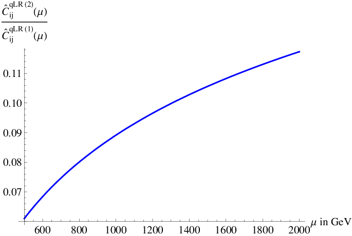
Figure 4: Relative importance of the two-loop corrections as a function of the matching scale μ\mu. We see that the two-loop contribution is approximately +9% of the one-loop contribution for μ=MSUSY=1​TeV\mu=M_{\rm SUSY}=1\,{\rm TeV}. C^f​iq​L​R\hat{C}_{fi}^{q\,LR} is defined in Eq. (36).
 

In this section we study the numerical importance of our two-loop corrections and the reduced matching scale dependence compared to the one-loop result.

The matching scale dependence, as shown in Fig. 3 for SUSY masses of 1 TeV, is significantly reduced as expected from the previous subsection. Note that the relative importance of the NLO result is to a very good approximation independent of the size of Δi​jq​L​R\Delta^{q\,LR}_{ij}.

The relative importance of the two-loop contribution to C^i​jq​L​R​(μ)\hat{C}^{q\;LR}_{ij}(\mu) is shown in Fig. 4 as a function of the matching scale μ\mu. For SUSY masses of 1 TeV the αs2\alpha_{s}^{2} corrections lead to a constructive contribution of approximately 9%9\% compared to the one-loop result that is in agreement with Ref. [16]. Again, the relative importance of the NLO result is to a very good approximation independent of the size of Δi​jq​L​R\Delta^{q\,LR}_{ij}.

IV.6 Transition to the decoupling limit

While the two-loop contributions calculated in this section are obtained in the approximation p=mq=0p=m_{q}=0, the results given in Sec. IV.3 still contain all powers v/MSUSYv/M_{\rm{SUSY}} implicitly via the squark mixing matrices Wq~W^{\tilde{q}} and the physical squark masses mq~sm_{\tilde{q}_{s}} involved. The transition to the decoupling limit, in which all chirally enhanced corrections can be resummed analytically, can be done by the following prescription.

In all parts of the genuine two-loop contributions listed above (Eq. (24)–Eq. (30)) only two mixing matrices occur, except in Eq. (24) and Eq. (IV.3). Eq. (24) contains the following combinations of mixing matrices and a loop-function ff which depends on squarks masses mq~sm_{\tilde{q}_{s}} and mq~tm_{\tilde{q}_{t}}

∑s,t=16∑j=13Wf​td~Wj+3,td~⋆Wi+3,sd~⋆Wj+3,sd~f(xs2,xt2).\sum\limits_{s,t=1}^{6}\sum\limits_{j=1}^{3}W_{ft}^{\tilde{d}}\,W_{j+3,t}^{\tilde{d}\star}\,W_{i+3,s}^{\tilde{d}\star}\,W_{j+3,s}^{\tilde{d}}\,f(x_{s}^{2},\,x_{t}^{2})\,. (43)

Note that in the decoupling limit, the squark with index ss in Eq. (43) must be a linear combination of right-handed squark only, since otherwise at least two chirality changes (two insertions of Δi​jd​L​R\Delta^{d\,LR}_{ij}) would be necessary. Thus we can replace

Wi+3,sd~⋆Wj+3,sd~→Γik⋆D​RΓj​kD​R=Λd​R​Rk​j​iandxs2→xR​k2,W_{i+3,s}^{\tilde{d}\star}\,W_{j+3,s}^{\tilde{d}}\,\to\;\Gamma^{ik\star}_{DR}\Gamma^{jk}_{DR}=\Lambda^{d\,RR}_{k\,ji}\qquad{\rm and}\qquad x_{s}^{2}\;\to\;x_{Rk}^{2}\,, (44)

where kk only runs from 1 to 3 and we defined

xL⁡(R)​k2=mq~kL⁡(R)2mg~2.x_{L(R)k}^{2}=\dfrac{m^{2}_{\tilde{q}_{k}^{L(R)}}}{m_{\tilde{g}}^{2}}\,. (45)

The resulting expression

∑t=16∑k,j=13Wf​td~Wj+3,td~⋆Λk​j​id​R​Rf(xR​k2,xt2)\sum\limits_{t=1}^{6}\sum\limits_{k,j=1}^{3}W_{ft}^{\tilde{d}}\,W_{j+3,t}^{\tilde{d}\star}\,\Lambda^{d\,RR}_{k\,ji}\,f(x_{Rk}^{2},\,x_{t}^{2}) (46)

can now be expanded in powers of v/MSUSYv/M_{\rm SUSY} which amounts at leading order to the replacement

∑t=16Wf​td~Wj+3,td~⋆f(…,xt2)→∑m,n,j′,j′′=13Λm​f​j′′d​L​LΔj′′​j′d​L​RΛn​j′​jd​R​Rf⁡(…,xL​m2)−f⁡(…,xR​n2)mq~mL2−mq~nR2,\sum\limits_{t=1}^{6}W_{ft}^{\tilde{d}}W_{j+3,t}^{\tilde{d}\star}f(\ldots\,,x_{t}^{2})\;\to\;\sum\limits_{m,n,j^{\prime},j^{\prime\prime}=1}^{3}\Lambda_{m\;fj^{\prime\prime}}^{d\,LL}\Delta_{j^{\prime\prime}j^{\prime}}^{d\,LR}\Lambda_{n\;j^{\prime}j}^{d\,RR}\dfrac{f(...\,,x_{Lm}^{2})-f(...\,,x_{Rn}^{2})}{m^{2}_{\tilde{q}_{m}^{L}}-m^{2}_{\tilde{q}_{n}^{R}}}\,, (47)

where the dots represent possible additional dependences on squark masses. Now we apply Eq. (47) to Eq. (46) and use

∑j=13Λm​f​jd⁡(L​L)​R​R​Λn​j​id⁡(L​L)​R​R=Λm​f​id⁡(L​L)​R​R​δm​n.\sum\limits_{j=1}^{3}\Lambda_{m\;fj}^{d\,(LL)RR}\Lambda_{n\;ji}^{d\,(LL)RR}=\Lambda_{m\;fi}^{d\,(LL)RR}\delta_{mn}\,. (48)

The final result for Eq. (43) in the decoupling limit is then

∑m,n,j′,j′′=13Λm​f​j′′d​L​L​Δj′′​j′d​L​R​Λn​j′​id​R​R​f⁡(xR​n2,xL​m2)−f⁡(xR​n2,xR​n2)mq~mL2−mq~nR2.\sum\limits_{m,n,j^{\prime},j^{\prime\prime}=1}^{3}\Lambda_{m\;fj^{\prime\prime}}^{d\,LL}\Delta_{j^{\prime\prime}j^{\prime}}^{d\,LR}\Lambda_{n\;j^{\prime}i}^{d\,RR}\,\dfrac{f(x_{Rn}^{2},x_{Lm}^{2})-f(x_{Rn}^{2},x_{Rn}^{2})}{m^{2}_{\tilde{q}_{m}^{L}}-m^{2}_{\tilde{q}_{n}^{R}}}\,. (49)

For Eq. (IV.3) a similar procedure works. It contains the following combination of mixing matrices with a loop function depending on three different squark masses with the indices ss, tt, and s′s^{\prime}

∑s,t,s′=16∑j,j′=13Wf​sd~(Wj′+3,sd~⋆Wj′+3,td~Wj​td~⋆Wj​s′d~+Wj′​sd~⋆Wj′​td~Wj+3,td~⋆Wj+3,s′d~)Wi+3,s′d~⋆f(xs2,xt2,xs′2).\sum\limits_{s,t,s^{\prime}=1}^{6}\sum\limits_{j,j^{\prime}=1}^{3}{W_{fs}^{\tilde{d}}\left({W_{j^{\prime}+3,s}^{\tilde{d}\star}W_{j^{\prime}+3,t}^{\tilde{d}}W_{jt}^{\tilde{d}\star}W_{js^{\prime}}^{\tilde{d}}+W_{j^{\prime}s}^{\tilde{d}\star}W_{j^{\prime}t}^{\tilde{d}}W_{j+3,t}^{\tilde{d}\star}W_{j+3,s^{\prime}}^{\tilde{d}}}\right)W_{i+3,s^{\prime}}^{\tilde{d}\star}}\,f(x_{s}^{2},x_{t}^{2},x_{s^{\prime}}^{2})\,. (50)

Note that the first term in Eq. (50) vanishes in the decoupling limit since it necessarily involves multiple chirality flips. For the second term two replacements analogous to Eq. (44) have to be performed, and after using two times the relation in Eq. (48) the decoupling limit of Eq. (50) reads

∑m,n,j′,j′′=13Λm​f​j′′d​L​L​Δj′′​j′d​L​R​Λn​j′​id​R​R​f⁡(xL​m2,xL​m2,xR​n2)−f⁡(xL​m2,xR​n2,xR​n2)mq~mL2−mq~nR2.\sum\limits_{m,n,j^{\prime},j^{\prime\prime}=1}^{3}\!\!\!\Lambda_{m\;fj^{\prime\prime}}^{d\,LL}\Delta_{j^{\prime\prime}j^{\prime}}^{d\,LR}\Lambda_{n\;j^{\prime}i}^{d\,RR}\,\dfrac{f(x_{Lm}^{2},x_{Lm}^{2},x_{Rn}^{2})-f(x_{Lm}^{2},x_{Rn}^{2},x_{Rn}^{2})}{m^{2}_{\tilde{q}_{m}^{L}}-m^{2}_{\tilde{q}_{n}^{R}}}\,. (51)

This result involves the same combination of mixing matrices as the one in Eq. (49).

To all other parts of Cf​iC_{fi} the rule in Eq. (47) can be applied directly to obtain the corresponding expression in the decoupling limit.

V Relations between quark masses and the MSSM Yukawa couplings at NLO

Beyond one-loop Eq. (11) and Eq. (12) for the determination of YdY^{d} can easily be generalized to higher loop orders because the chirality changing self-energy (and also the resulting Wilson coefficient) is still proportional to one element Δi​jd​L​R\Delta^{d\;LR}_{ij} in the decoupling limit, as shown in Sec. IV.6. However, since we are dealing with order one corrections, we must specify how we count contributions at higher loop orders in αs\alpha_{s}. Cf​iq​L​R​(1)C_{fi}^{q\,LR\,\left(1\right)} is proportional αs​tan⁡β\alpha_{s}\tan\beta and Cf​iq​L​R​(2)C_{fi}^{q\;LR\;\left(2\right)} is proportional to αs2​tan⁡β\alpha_{s}^{2}\tan\beta. Here, tan⁡β\tan\beta stands schematically for a chiral enhancement factor, also including Ai​jq/(Yi​jq​MSUSY)A^{q}_{ij}/(Y^{q}_{ij}M_{\rm{SUSY}}). We will count αs​tan⁡β\alpha_{s}\tan\beta as order one and thus αs2​tan⁡β\alpha_{s}^{2}\tan\beta as order αs\alpha_{s}. Since Cf​iq​L​L,R​RC_{fi}^{q\,LL,RR} is not chirally enhanced, the only relevant term in our approximation (of order αs\alpha_{s}) is the one-loop contribution. Thus, Cf​iq​L​L,R​RC_{fi}^{q\,LL,RR} is always understood to be the one-loop contribution proportional to αs\alpha_{s}.

To derive the relation between the quark masses and the Yukawa couplings of the MSSM superpotential at NLO we also need to specify the renormalization scheme used for the matching procedure. Let us explicitly denote the renormalization scheme for the quantities in the matching condition Eq. (11) (at the scale mSUSYm_{\rm SUSY}) which is important at NLO:

vq​Yeffqi​MS¯=mqiMS¯=(vq​Ytreeqi​MS¯+Ci​i​MS¯q​L​R​(1)+Ci​iq​L​R​(2))×(1+12​(Ci​iq​L​L+Ci​iq​R​R)).v_{q}Y^{q_{i}\,\overline{\rm MS}}_{\rm{eff}}=m_{q_{i}}^{\overline{\rm MS}}=\left(v_{q}Y^{q_{i}\,\overline{\rm MS}}_{\rm tree}+C_{ii\,\overline{\rm MS}}^{q\,LR\,(1)}+C_{ii}^{q\,LR\,(2)}\right)\times\left(1+\dfrac{1}{2}\left({C_{ii}^{q\,LL}+C_{ii}^{q\,RR}}\right)\right)\,. (52)

Again, Ytreeqi​MS¯Y^{q_{i}\,\overline{\rm MS}}_{\rm tree} is the Wilson coefficient induced via the Yukawa coupling of the MSSM. This means at the matching scale it is given by:

Ytreeqi​MS¯​(μSUSY)=YMS¯qi​(μSUSY)=(1+αs4​π​CF)​YDR¯qi​(μSUSY).Y^{q_{i}\,\overline{\rm MS}}_{\rm tree}\left(\mu_{\rm SUSY}\right)=Y^{q_{i}}_{\overline{\rm MS}}\left(\mu_{\rm SUSY}\right)=\left(1+\frac{\alpha_{s}}{4\pi}C_{F}\right)Y^{q_{i}}_{\overline{{\rm DR}}}\left(\mu_{\rm SUSY}\right)\,. (53)

In our counting in αs\alpha_{s} and tan⁡β\tan\beta the renormalization scheme for Ci​iq​L​LC_{ii}^{q\,LL} and Ci​iq​R​RC_{ii}^{q\,RR} is irrelevant. Note that the quark mass mqim_{q_{i}} is understood to be evaluated at the matching scale. Further, one should recall from the last section that despite the fact that we renormalized Ci​iq​L​RC^{q\,LR}_{ii} in the MS¯\overline{\rm MS} scheme, it contains parameters given in the DR¯\overline{\rm DR} scheme, e.g. Yq~i=YDR¯qiY^{\tilde{q}_{i}}=Y^{q_{i}}_{\overline{\rm DR}}. Since we are interested in Yq~iY^{\tilde{q}_{i}}, the Yukawa coupling of the MSSM superpotential, we must express Ytreeqi​MS¯Y^{q_{i}\,\overline{\rm MS}}_{\rm tree} in Eq. (52) in terms of YDR¯q~iY^{\tilde{q}_{i}}_{\overline{\rm DR}} via Eq. (53) so that we can solve for YDR¯qiY^{q_{i}}_{\overline{\rm DR}}.

In conclusion we arrive at the NLO generalization (order αs2​tan⁡β\alpha_{s}^{2}\tan\beta) of Eq. (11):

YDR¯di=mdiMS¯−C^i​i​Yid​L​Rvd​(1+αs4​π​CF+tan⁡β​ϵ^id),Y^{d_{i}}_{\overline{{\rm DR}}}=\dfrac{m_{d_{i}}^{\overline{{\rm MS}}}-\hat{C}_{ii\,\cancel{Y_{i}}}^{d\,LR}}{v_{d}\left({1+\dfrac{\alpha_{s}}{4\pi}C_{F}+\tan\beta\hat{\epsilon}_{i}^{d}}\right)}\,, (54)

with C^f​iq​L​R\hat{C}_{fi}^{q\,LR} defined in Eq. (36) and the corresponding equation for ϵ^id\hat{\epsilon}_{i}^{d}. Here ϵid⁡(1)\epsilon_{i}^{d(1)} and ϵid⁡(2)\epsilon_{i}^{d\,(2)} are defined in direct analogy to Eq. (13). Further, the Wilson coefficients appearing here are assumed to be in the decoupling limit. Eq. (54) constitutes the NLO determination of the Yukawa coupling of the superpotential. When later inserting the Yukawa coupling into the Wilson coefficients, one has to use this relation99 9 The generalization to the CKM matrix can be achieved following the procedure of [10, 11, 7].

The electroweak contributions (involving charginos and neutralinos) to the relation between the quark masses and the Yukawa couplings are in most regions of the parameter space subleading compared to the strong contributions. However, the LO electroweak corrections are easily as large as the NLO SQCD corrections and should be included in a numerical analysis. This can be achieved by simply adding the corresponding contributions to C^i​i​Yid​L​R\hat{C}_{ii\,\cancel{Y_{i}}}^{d\,LR} and ϵ^id\hat{\epsilon}_{i}^{d} in Eq. (54).

VI Effective Higgs vertices

To derive the effective Higgs-quark-quark couplings1010 10 In principle also the renormalization of the Higgs potential should be addressed. Our derivation of chirally enhanced flavor effects does not depend on the specific relations between Higgs self-couplings and their masses. Since no chirally enhanced effects occur in the Higgs sector, it is consistent to use the tree-level values for the Higgs parameters. However, one can as well use the NLO values for the Higgs masses and mixing angles which might be even better from the numerical point of view. we have to assume that the external momenta (flowing through the Higgs-quark-quark vertex) are much smaller than the masses of the virtual SUSY particles running in the loop. This assumption limits the applicability of the resulting Feynman rules. If mH0,mA0,mH±≪MSUSYm_{H^{0}},m_{A^{0}},m_{H^{\pm}}\ll M_{\rm{SUSY}} (H0,A0H^{0},A^{0}, and H±H^{\pm} denote the neutral CP-even, CP-odd and the charged Higgs boson, respectively), the effective Feynman rules can be used for the calculation of all flavor-observables (also if the Higgs is propagating in a loop) and for processes with a Higgs on the mass shell. If the hierarchy mH0,mA0,mH±≪MSUSYm_{H^{0}},m_{A^{0}},m_{H^{\pm}}\ll M_{\rm{SUSY}} is not satisfied the effective Higgs vertices can still be used for processes in which the momentum flow through the Higgs-quark-quark vertex is small compared to MSUSYM_{\rm{SUSY}} which is true for all low-energy flavor observables with tree-level Higgs exchange (like Bd,s→μ+​μ−B_{d,s}\to\mu^{+}\mu^{-}, B+→τ+​νB^{+}\to\tau^{+}\nu or the double Higgs penguin contributing to Δ​F=2\Delta F=2 processes).

As discussed in the Introduction we use an effective field theory approach in our study of the Higgs-quark-quark couplings which simplifies the calculations significantly. This means that we match the MSSM on the 2HDM of type III at the scale MSUSYM_{\rm SUSY} rather than calculating the Higgs-quark-quark coupling within the MSSM.

Let as first consider the effective Lagrangian of a general 2HDM (including Higgs-quark-quark couplings and kinetic terms):

ℒe​f​f=Q¯f​La((Yf​i​ewd​tree+Ef​id​ew)ϵb​aHdb⋆−Ef​i′d​ewHua)di​R+Q¯f​La((Yf​i​ewu​tree+Ef​iu​ew)ϵa​bHub⋆−Ef​i′u​ewHda)ui​R+d¯f​R​i​∂​(δf​i−Rf​id​ew)​di​R+u¯f​R​i​∂​(δf​i−Rf​iu​ew)​ui​R+Q¯f​La​i​∂​(δf​i−Lf​iq​ew)​Qi​La,\begin{array}[]{l}{\cal L}^{eff}=\bar{Q}_{f\;L}^{a}\left({\left({Y_{fi\,{\rm ew}}^{d\,{\rm tree}}+E_{fi}^{d\;{\rm ew}}}\right)\epsilon_{ba}H_{d}^{b\star}-E_{fi}^{\prime d\;{\rm ew}}H_{u}^{a}}\right)d_{i\;R}\\ \phantom{L^{eff}=}+\bar{Q}_{f\;L}^{a}\left({\left({Y_{fi\,{\rm ew}}^{u\,{\rm tree}}+E_{fi}^{u\;{\rm ew}}}\right)\epsilon_{ab}H_{u}^{b\star}-E_{fi}^{\prime u\;{\rm ew}}H_{d}^{a}}\right)u_{i\;R}\\ \phantom{L^{eff}=}+\bar{d}_{f\;R}i\cancel{\partial}\left({\delta_{fi}-R_{fi}^{d\,{\rm ew}}}\right)d_{i\;R}+\bar{u}_{f\;R}i\cancel{\partial}\left({\delta_{fi}-R_{fi}^{u\,{\rm ew}}}\right)u_{i\;R}\\ \phantom{L^{eff}=}+\bar{Q}_{f\;L}^{a}i\cancel{\partial}\left({\delta_{fi}-L_{fi}^{q\,{\rm ew}}}\right)Q_{i\;L}^{a}\,,\end{array} (55)

where adding the Hermitian conjugate of the terms involving Higgs fields is implicitly meant. The Higgs doublets are defined as

Hd=(Hd1Hd2)=(Hd0Hd−),Hu=(Hu1Hu2)=(Hu+Hu0).\begin{array}[]{l}{H_{d}}=\left({\begin{array}[]{*{20}{c}}{H_{d}^{1}}\\ {H_{d}^{2}}\end{array}}\right)=\left({\begin{array}[]{*{20}{c}}{H_{d}^{0}}\\ {H_{d}^{-}}\end{array}}\right)\,,\\ {H_{u}}=\left({\begin{array}[]{*{20}{c}}{H_{u}^{1}}\\ {H_{u}^{2}}\end{array}}\right)=\left({\begin{array}[]{*{20}{c}}{H_{u}^{+}}\\ {H_{u}^{0}}\end{array}}\right)\,.\end{array} (56)

In Eq. (55) aa, bb denote S​U​(2)LSU(2)_{L} - indices and ϵa​b\epsilon_{ab} is the two-dimensional antisymmetric tensor with ϵ12=−1\epsilon_{12}=-1. We introduced the holomorphic couplings Ef​iq​ewE^{q\,{\rm ew}}_{fi}, the nonholomorphic couplings Ef​i′q​ewE^{\prime q\,{\rm ew}}_{fi} (q=u,dq=u,d), and the contributions to the kinetic terms Rf​id,u​ewR_{fi}^{d,u\,{\rm ew}} and Lf​iq​ewL_{fi}^{q\,{\rm ew}}. Here the superscript “ew” refers to the fact that these terms are given in a weak-interaction eigenbasis. In Eq. (55) we already anticipated the MSSM where the terms E(′)qewf​iE^{(\prime)q\,{\rm ew}}_{fi}, Lf​iq​ewL_{fi}^{q\,{\rm ew}} and Rf​iq​ewR_{fi}^{q\,{\rm ew}} are loop induced but Yf​i​ewu​treeY^{u\,{\rm tree}}_{fi\,{\rm ew}} and Yf​i​ewd​treeY^{d\,{\rm tree}}_{fi\,{\rm ew}} are generated at tree level via the MSSM Yukawa couplings1111 11 In principle, without knowing anything about the MSSM, the holomorphic corrections could be absorbed into an effective Yukawa coupling (and also the corrections to the kinetic terms Rf​id,u​ewR_{fi}^{d,u\,{\rm ew}} and Lf​iq​ewL_{fi}^{q\,{\rm ew}} would not be physical). However, once we go back to the MSSM with the SUSY breaking terms as input parameters, also the holomorphic corrections become physical..

To connect the effective theory to the MSSM we go to the super-CKM basis, in which the Yukawa couplings are diagonal, by rotating the fields

qj​L,R→Uj​iq​L,R⁡(0)​qi​L,R,q_{j\;L,R}\to U_{ji}^{q\;L,R\left(0\right)}q_{i\;L,R}\,, (57)

such that

Uk​fqL(0)⋆Yk​j​ewq​treeUj​iq​R​(0)=Yqitreeδf​i.U_{kf}^{q\;L\left(0\right)\star}Y_{kj\,{\rm ew}}^{q\,{\rm tree}}U_{ji}^{q\;R\left(0\right)}=Y^{q_{i}}_{\rm tree}\delta_{fi}\,. (58)

We now break the electroweak symmetry and write the effective Lagrangian in component form:

ℒe​f​f=u¯f​LVf​j(0)((Ytreedjδj​i+Ej​id)Hd2⋆−Ej​i′dHu1)di​R+d¯f​LVj​f(0)⋆((Ytreeujδj​i+Ej​iu)Hu1⋆−Ej​i′uHd2)ui​R−d¯f​L((Ytreedfδf​i+Ef​id)Hd1⋆+Ef​i′dHu2)di​R−u¯f​L((Ytreeufδf​i+Ef​iu)Hu2⋆+Ef​i′uHd1)ui​R+d¯f​R​i​∂​(δf​i−Rf​id)​di​R+u¯f​R​i​∂​(δf​i−Rf​iu)​ui​R+d¯f​L​i​∂​(δf​i−Lf​id)​di​L+u¯f​L​i​∂​(δf​i−Lf​iu)​ui​L−d¯f​L​((Ytreedf​δf​i+Ef​id)​vd+Ef​i′d​vu)​di​R−u¯f​L​((Ytreeuf​δf​i+Ef​iu)​vu+Ef​i′u​vd)​ui​R,\begin{array}[]{l}{\cal L}^{eff}=\bar{u}_{f\;L}V_{fj}^{\left(0\right)}\left({\left({Y_{\rm tree}^{d_{j}}\delta_{ji}+E_{ji}^{d}}\right)H_{d}^{2\star}-E_{ji}^{\prime d}H_{u}^{1}}\right)d_{i\;R}\\ \phantom{L^{eff}=}+\bar{d}_{f\;L}V_{jf}^{\left(0\right)\star}\left({\left({Y_{\rm tree}^{u_{j}}\delta_{ji}+E_{ji}^{u}}\right)H_{u}^{1\star}-E_{ji}^{\prime u}H_{d}^{2}}\right)u_{i\;R}\\ \phantom{L^{eff}=}-\bar{d}_{f\;L}\left({\left({Y_{\rm tree}^{d_{f}}\delta_{fi}+E_{fi}^{d}}\right)H_{d}^{1\star}+E_{fi}^{\prime d}H_{u}^{2}}\right)d_{i\;R}\\ \phantom{L^{eff}=}-\bar{u}_{f\;L}\left({\left({Y_{\rm tree}^{u_{f}}\delta_{fi}+E_{fi}^{u}}\right)H_{u}^{2\star}+E_{fi}^{\prime u}H_{d}^{1}}\right)u_{i\;R}\\ \phantom{L^{eff}=}+\bar{d}_{f\;R}i\cancel{\partial}\left({\delta_{fi}-R_{fi}^{d}}\right)d_{i\;R}+\bar{u}_{f\;R}i\cancel{\partial}\left({\delta_{fi}-R_{fi}^{u}}\right)u_{i\;R}\\ \phantom{L^{eff}=}+\bar{d}_{f\;L}i\cancel{\partial}\left({\delta_{fi}-L_{fi}^{d}}\right)d_{i\;L}+\bar{u}_{f\;L}i\cancel{\partial}\left({\delta_{fi}-L_{fi}^{u}}\right)u_{i\;L}\\ \phantom{L^{eff}=}-\bar{d}_{f\;L}\left({\left({Y_{\rm tree}^{d_{f}}\delta_{fi}+E_{fi}^{d}}\right)v_{d}+E_{fi}^{\prime d}v_{u}}\right)d_{i\;R}\\ \phantom{L^{eff}=}-\bar{u}_{f\;L}\left({\left({Y_{\rm tree}^{u_{f}}\delta_{fi}+E_{fi}^{u}}\right)v_{u}+E_{fi}^{\prime u}v_{d}}\right)u_{i\;R}\,,\\ \end{array} (59)

where V(0)=UuL(0)†Ud​L​(0)V^{\left(0\right)}=U^{u\;L\left(0\right){\dagger}}U^{d\;L\;\left(0\right)} is not the physical CKM matrix, but rather the CKM matrix generated by the misalignment of the Yukawa couplings. Adding the Hermitian conjugate of the mass terms and the terms involving Higgs fields is tacitly understood. The terms

Ef​iq=Uk​fqL(0)⋆Ek​jq​ewUj​iq​R​(0)Ef​i′q=Uk​fqL(0)⋆Ek​j′q​ewUj​iq​R​(0)Rf​iq=Uk​fqR(0)⋆Rk​jq​ewUj​iq​R​(0)Lf​id=Uk​fdL(0)⋆Lk​jq​ewUj​id​L​(0)Lf​iu=Uk​fuL(0)⋆Lk​jq​ewUj​iu​L​(0)=Vf​k(0)Lk​jdVi​j(0)⋆\begin{array}[]{l}E_{fi}^{q}=U_{kf}^{q\;L\left(0\right)\star}E_{kj}^{q\,{\rm ew}}U_{ji}^{q\;R\left(0\right)}\\ E_{fi}^{\prime q}=U_{kf}^{q\;L\left(0\right)\star}E_{kj}^{\prime q\,{\rm ew}}U_{ji}^{q\;R\left(0\right)}\\ R_{fi}^{q}=U_{kf}^{q\;R\left(0\right)\star}R_{kj}^{q\,{\rm ew}}U_{ji}^{q\;R\left(0\right)}\\ L_{fi}^{d}=U_{kf}^{d\;L\left(0\right)\star}L_{kj}^{q\,{\rm ew}}U_{ji}^{d\;L\left(0\right)}\\ L_{fi}^{u}=U_{kf}^{u\;L\left(0\right)\star}L_{kj}^{q\,{\rm ew}}U_{ji}^{u\;L\left(0\right)}=V_{fk}^{\left(0\right)}L_{kj}^{d}V_{ij}^{\left(0\right)\star}\\ \end{array} (60)

are now given in the super-CKM basis. Note that this is the same basis as the one in which the effective Lagrangian of Eq. (2) is given (and the same basis in which we calculated the MSSM contributions to the Wilson coefficients). Thus, comparing the last four lines of Eq. (59) to Eq. (2) we have the following relation between the Wilson coefficients and the terms of the 2HDM III Lagrangian (at an arbitrary loop order):

Edf​i=Cf​i​Ad​L​Rvd,E′df​i=Cf​i′d​L​Rvu,Euf​i=Cf​i​Au​L​Rvu,E′uf​i=Cf​i′u​L​Rvd,Lqf​i=Cq​L​Lf​i,Rqf​i=Cq​R​Rf​i.\begin{array}[]{l}E^{d}_{fi}\,=\,\dfrac{C^{d\,LR}_{fi\,A}}{v_{d}}\,,\hskip 42.67912ptE^{\prime d}_{fi}\,=\,\dfrac{C^{\prime\,d\,LR}_{fi}}{v_{u}}\,,\\ E^{u}_{fi}\,=\,\dfrac{C^{u\,LR}_{fi\,A}}{v_{u}}\,,\hskip 42.67912ptE^{\prime u}_{fi}\,=\,\dfrac{C^{\prime\,u\,LR}_{fi}}{v_{d}}\,,\\ L^{q}_{fi}\,=C^{q\,LL}_{fi}\,,\hskip 42.67912ptR^{q}_{fi}\,=C^{q\,RR}_{fi}\,.\end{array} (61)

Now we want to go to the physical basis with flavor diagonal mass terms and canonical kinetic terms. As a first step we render the kinetic terms canonical by a field redefinition:

qi​L→(δi​j+12​Li​jq)​qj​L,qi​R→(δi​j+12​Ri​jq)​qj​R.\begin{array}[]{l}q_{i\;L}\to\left({\delta_{ij}+\dfrac{1}{2}L_{ij}^{q}}\right)q_{j\;L}\,,\\ q_{i\;R}\to\left({\delta_{ij}+\dfrac{1}{2}R_{ij}^{q}}\right)q_{j\;R}\,.\\ \end{array} (62)

Consider now the quark mass matrices. The redefinition of the fields in Eq. (62) also leads to a shift in down-quark mass matrix so that it is now given by

mf​id=(E^^f​id+Y^^f​id​tree)​vd+vu​E^^f​i′d=C^^f​id​L​R+vd​Y^^f​id​tree,mf​iu=(E^^f​iu+Y^^f​iu​tree)​vu+vd​E^^f​i′u=C^^f​iu​L​R+vu​Y^^f​iu​tree,\begin{array}[]{l}m_{fi}^{d}=\left({\hat{\hat{E}}_{fi}^{d}+\hat{\hat{Y}}_{fi}^{d\,{\rm tree}}}\right)v_{d}+v_{u}\hat{\hat{E}}_{fi}^{\prime d}=\hat{\hat{C}}_{fi}^{d\;LR}+v_{d}\hat{\hat{Y}}_{fi}^{d\,{\rm tree}}\,,\\ m_{fi}^{u}=\left({\hat{\hat{E}}_{fi}^{u}+\hat{\hat{Y}}_{fi}^{u\,{\rm tree}}}\right)v_{u}+v_{d}\hat{\hat{E}}_{fi}^{\prime u}=\hat{\hat{C}}_{fi}^{u\;LR}+v_{u}\hat{\hat{Y}}_{fi}^{u\,{\rm tree}}\,,\end{array} (63)

where we have defined

E^^f​i(′)q=Ef​i(′)q+12∑j=13(Lf​jqEj​i(′)q+Ef​j(′)qRj​iq),Y^^f​iq​tree=Ytreeqi​δf​i+12​∑j=13(Cf​jq​L​L​Ytreeqi​δj​i+Ytreeqf​δf​j​Cj​iq​R​R),C^^f​iq​L​R=Cf​iq​L​R+12​∑j=13(Cf​jq​L​L​Cj​iq​L​R+Cf​jq​L​R​Cj​iq​R​R).\begin{array}[]{l}\hat{\hat{E}}_{fi}^{(\prime)q}=E_{fi}^{(\prime)q}+\dfrac{1}{2}\sum\limits_{j=1}^{3}{\left({L_{fj}^{q}E_{ji}^{(\prime)q}+E_{fj}^{(\prime)q}R_{ji}^{q}}\right)}\,,\\ \hat{\hat{Y}}_{fi}^{q\,{\rm tree}}=Y^{q_{i}}_{{\rm tree}}\delta_{fi}+\dfrac{1}{2}\sum\limits_{j=1}^{3}{\left({C_{fj}^{q\,LL}Y^{q_{i}}_{\rm tree}\delta_{ji}+Y^{q_{f}}_{\rm tree}\delta_{fj}C_{ji}^{q\,RR}}\right)}\,,\\ \hat{\hat{C}}_{fi}^{q\;LR}=C_{fi}^{q\;LR}+\dfrac{1}{2}\sum\limits_{j=1}^{3}{\left({C_{fj}^{q\,LL}C_{ji}^{q\;LR}+C_{fj}^{q\;LR}C_{ji}^{q\,RR}}\right)}\,.\\ \end{array} (64)

Note that the quantities with a double hat contain also the contributions from flavor-changing LL and RR Wilson coefficients, while the quantities with one hat (see Eq. (36) and Eq. (80)) only contain the flavor-conserving LL and RR Wilson coefficients.

We now diagonalize the quark mass matrices by a bi-unitary transformation

Uk​fqL⋆mk​jqUj​iq​R=mqiδf​i,U_{kf}^{q\,L\star}m_{kj}^{q}U_{ji}^{q\,R}=m_{q_{i}}\delta_{fi}\,, (65)

where the rotation matrices

Uq​L=(1m12qmq2m13qmq3−m12q⋆mq21m23qmq3−m13q⋆mq3+m12q⋆m23q⋆mq2​mq3−m23q⋆mq31),Uq​R=(1m21q⋆mq2m31q⋆mq3−m21qmq21m32q⋆mq3−m31qmq3+m32q​m21qmq2​mq3−m32q⋆mq31)U^{q\,L}=\left({\begin{array}[]{*{20}c}1&{\dfrac{{m_{12}^{q}}}{{m_{q_{2}}}}}&{\dfrac{{m_{13}^{q}}}{{m_{q_{3}}}}}\\ {\dfrac{{-m_{12}^{q\star}}}{{m_{q_{2}}}}}&1&{\dfrac{{m_{23}^{q}}}{{m_{q_{3}}}}}\\ {\dfrac{{-m_{13}^{q\star}}}{{m_{q_{3}}}}+\dfrac{{m_{12}^{q\star}m_{23}^{q\star}}}{{m_{q_{2}}m_{q_{3}}}}}&{\dfrac{{-m_{23}^{q\star}}}{{m_{q_{3}}}}}&1\\ \end{array}}\right),\;\;\;U^{q\,R}=\left({\begin{array}[]{*{20}c}1&{\dfrac{{m_{21}^{q\star}}}{{m_{q_{2}}}}}&{\dfrac{{m_{31}^{q\star}}}{{m_{q_{3}}}}}\\ {\dfrac{{-m_{21}^{q}}}{{m_{q_{2}}}}}&1&{\dfrac{{m_{32}^{q\star}}}{{m_{q_{3}}}}}\\ {\dfrac{{-m_{31}^{q}}}{{m_{q_{3}}}}+\dfrac{{m_{32}^{q}m_{21}^{q}}}{{m_{q_{2}}m_{q_{3}}}}}&{\dfrac{{-m_{32}^{q\star}}}{{m_{q_{3}}}}}&1\\ \end{array}}\right) (66)

are obtained from a perturbative diagonalization of the quark mass matrix1212 12 Note that these rotations are identical to the ones obtained in the diagrammatic approach (see Ref. [20] for details)..

Switching to the physical basis in which the quark mass matrices are diagonal, these rotations modify the effective Lagrangian as follows [20]:

ℒe​f​f=u¯f​LUk​fuL⋆Vk​k′(0)(mk′​jdvdHd2⋆−E^^k′​j′d(Hu1+tan(β)Hd2⋆))Uj​id​Rdi​R+d¯f​LUk​fdL⋆Vk′​k(0)⋆(mk′​juvuHu1⋆−E^^k′​j′u(Hd2+cot(β)Hu1⋆))Uj​id​Rui​R−d¯f​LUk​fdL⋆(mk​jdvdHd1⋆+E^^k​j′d(Hu2−tan(β)Hd1⋆))Uj​id​Rdi​R−u¯f​LaUk​fuL⋆(mk​juvuHu2⋆+E^^k​j′u(Hd1−cot(β)Hu2⋆))Uj​iu​Rui​R+h.c.\displaystyle\begin{array}[]{l}\mathcal{L}^{eff}=\bar{u}_{f\;L}U_{kf}^{u\;L\star}V_{kk^{\prime}}^{\left(0\right)}\left({\dfrac{{m_{k^{\prime}j}^{d}}}{{v_{d}}}H_{d}^{2\star}-\hat{\hat{E}}_{k^{\prime}j}^{\prime d}\left({H_{u}^{1}+\tan\left(\beta\right)H_{d}^{2\star}}\right)}\right)U_{ji}^{d\;R}d_{i\;R}\\ \phantom{\mathcal{L}^{eff}=}+\bar{d}_{f\;L}U_{kf}^{d\;L\star}V_{k^{\prime}k}^{\left(0\right)\star}\left({\dfrac{{m_{k^{\prime}j}^{u}}}{{v_{u}}}H_{u}^{1\star}-\hat{\hat{E}}_{k^{\prime}j}^{\prime u}\left({H_{d}^{2}+\cot\left(\beta\right)H_{u}^{1\star}}\right)}\right)U_{ji}^{d\;R}u_{i\;R}\\ \phantom{\mathcal{L}^{eff}=}-\bar{d}_{f\;L}U_{kf}^{d\;L\star}\left({\dfrac{{m_{kj}^{d}}}{{v_{d}}}H_{d}^{1\star}+\hat{\hat{E}}_{kj}^{\prime d}\left({H_{u}^{2}-\tan\left(\beta\right)H_{d}^{1\star}}\right)}\right)U_{ji}^{d\;R}d_{i\;R}\\ \phantom{\mathcal{L}^{eff}=}-\bar{u}_{f\;L}^{a}U_{kf}^{u\;L\star}\left({\dfrac{{m_{kj}^{u}}}{{v_{u}}}H_{u}^{2\star}+\hat{\hat{E}}_{kj}^{\prime u}\left({H_{d}^{1}-\cot\left(\beta\right)H_{u}^{2\star}}\right)}\right)U_{ji}^{u\;R}u_{i\;R}\,+\,h.c.\\ \end{array}

where we skipped the mass terms and the kinetic terms. This can be further simplified by using the physical CKM matrix given by

Vf​i=Uj​fuL⋆Vj​k(0)Uk​id​L.V_{fi}=U_{jf}^{u\;L\star}V_{jk}^{\left(0\right)}U_{ki}^{d\;L}\,. (72)

In addition, we define the abbreviations

E~f​i′q=Uk​fqL⋆E^^k​j′qUj​iq​R=E^f​i′q−(0E^22′q​c^12q​L​RE^33′q​(c^13q​L​R−c^12q​L​R​c^23q​L​R)E^22′q​c^21q​L​R0E^33′q​c^23q​L​RE^33′q​(c^31q​L​R−c^32q​L​R​c^31q​L​R)E^33′q​c^32q​L​R0)f​i≡E^f​i′q−Δ​E^f​i′q.\displaystyle\begin{array}[]{l}\tilde{E}_{fi}^{\prime q}=U_{kf}^{q\;L\star}\hat{\hat{E}}_{kj}^{\prime q}U_{ji}^{q\;R}\\ \phantom{\tilde{E}_{fi}^{\prime q}}=\hat{E}_{fi}^{\prime q}-\left({\begin{array}[]{*{20}c}0&{\hat{E}_{22}^{\prime q}\hat{c}_{12}^{q\;LR}}&{\hat{E}_{33}^{\prime q}\left({\hat{c}_{13}^{q\;LR}-\hat{c}_{12}^{q\;LR}\hat{c}_{23}^{q\;LR}}\right)}\\ {\hat{E}_{22}^{\prime q}\hat{c}_{21}^{q\;LR}}&0&{\hat{E}_{33}^{\prime q}\hat{c}_{23}^{q\;LR}}\\ {\hat{E}_{33}^{\prime q}\left({\hat{c}_{31}^{q\;LR}-\hat{c}_{32}^{q\;LR}\hat{c}_{31}^{q\;LR}}\right)}&{\hat{E}_{33}^{\prime q}\hat{c}_{32}^{q\;LR}}&0\\ \end{array}}\right)_{fi}\\ \phantom{\tilde{E}_{fi}^{\prime q}}\equiv\hat{E}_{fi}^{\prime q}-\Delta\hat{E}_{fi}^{\prime q}\,.\end{array}

Note that in this expression only quantities with a single hat defined as

E^f​i(′)q=Ef​i(′)q+12(Lf​fqEf​i(′)q+Ef​i(′)qRi​iq)´,\hat{E}_{fi}^{(\prime)q}=E_{fi}^{(\prime)q}+\frac{1}{2}\left({L_{ff}^{q}E_{fi}^{(\prime)q}+E_{fi}^{(\prime)q}R_{ii}^{q}}\right)\,\textasciiacute, (80)

and c^i​jq​L​R\hat{c}^{q\;LR}_{ij} defined by combining Eq. (36) with

cj​iq​L​R=Cj​iq​L​Rmax⁡{mqj,mqi},c^{q\;LR}_{ji}\,=\,\dfrac{C_{ji}^{q\,LR}}{\max\{m_{q_{j}},m_{q_{i}}\}}\,, (81)

enter. This is in agreement with the finding of Ref. [23] that the effect of the flavor-changing LL and RR self-energies drops out in the effective Higgs vertices.

Finally, to arrive at the effective Feynman rules we project the fields Hu0H^{0}_{u} and Hd0H^{0}_{d} onto the physical components H0H^{0}, h0h^{0}, A0A^{0} and H±H^{\pm} as

Hu0\displaystyle H_{u}^{0} =\displaystyle= 12​(H0​sin⁡α+h0​cos⁡α+i​A0​cos⁡β),\displaystyle\frac{1}{\sqrt{2}}\left(H^{0}\sin\alpha+h^{0}\cos\alpha+iA^{0}\cos\beta\right)\,,
Hd0\displaystyle H_{d}^{0} =\displaystyle= 12​(H0​cos⁡α−h0​sin⁡α+i​A0​sin⁡β),\displaystyle\frac{1}{\sqrt{2}}\left(H^{0}\cos\alpha-h^{0}\sin\alpha+iA^{0}\sin\beta\right)\,,
Hu1⋆\displaystyle H_{u}^{1\star} =\displaystyle= cos⁡(β)​H−,\displaystyle\cos\left(\beta\right){H^{-}}\,,
Hd2\displaystyle H_{d}^{2} =\displaystyle= sin⁡(β)​H−.\displaystyle\sin\left(\beta\right){H^{-}}\,. (82)

Using Eq. (72), Eq. (VI), and Eq. (82), the effective Lagrangian in Eq. (VI) leads to the following effective Higgs-quark-quark Feynman rules1313 13 Note that some of the Higgs-quark-quark couplings are suppressed by a factor cos⁡β\cos\beta or sin⁡α\sin\alpha stemming from the Higgs mixing matrices. If one decides to keep these suppressed couplings, one should be aware of the fact that they receive proper vertex corrections in which the suppression factor does not occur and which are thus tan⁡β\tan\beta enhanced with respect to the tree-level couplings. Such enhanced corrections to the coupling of H±H^{\pm} to right-handed up quarks are important for b→s​γb\to s\gamma [36, 37]. shown in Fig. 5 (note that the CKM matrix VV in the charged Higgs coupling is the physical one):

Γuf​uiL​R​Hk0\displaystyle{\Gamma_{u_{f}u_{i}}^{LR\,H_{k}^{0}}} =\displaystyle= xuk(muivuδf​i−E~f​i′ucotβ)+xdk⋆E~f​i′u,\displaystyle x_{u}^{k}\left(\frac{m_{u_{i}}}{v_{u}}\delta_{fi}-\widetilde{E}_{fi}^{\prime u}\cot\beta\right)+x_{d}^{k\star}\widetilde{E}_{fi}^{\prime u}\,,
Γdf​diL​R​Hk0\displaystyle{\Gamma_{d_{f}d_{i}}^{LR\,H_{k}^{0}}} =\displaystyle= xdk(mdivdδf​i−E~f​i′dtanβ)+xuk⋆E~f​i′d,\displaystyle x_{d}^{k}\left(\frac{m_{d_{i}}}{v_{d}}\delta_{fi}-\widetilde{E}_{fi}^{\prime d}\tan\beta\right)+x_{u}^{k\star}\widetilde{E}_{fi}^{\prime d}\,,
Γuf​diL​R​H±\displaystyle{\Gamma_{u_{f}d_{i}}^{LR\,H^{\pm}}} =\displaystyle= ∑j=13sin⁡β​Vf​j​(mdivd​δj​i−E~j​i′d​tan⁡β),\displaystyle\sum\limits_{j=1}^{3}{\sin\beta\,V_{fj}\left(\frac{m_{d_{i}}}{v_{d}}\delta_{ji}-\widetilde{E}^{\prime d}_{ji}\tan\beta\right)\,,}
Γdf​uiL​R​H±\displaystyle{\Gamma_{d_{f}u_{i}}^{LR\,H^{\pm}}} =\displaystyle= ∑j=13cos⁡β​Vj​f⋆​(muivu​δj​i−E~j​i′u​tan⁡β),\displaystyle\sum\limits_{j=1}^{3}{\cos\beta\,V_{jf}^{\star}\left(\frac{m_{u_{i}}}{v_{u}}\delta_{ji}-\widetilde{E}^{\prime u}_{ji}\tan\beta\right)\,}\,, (83)

where for Hk0=(H0,h0,A0)H^{0}_{k}=(H^{0},h^{0},A^{0}) the coefficients xqkx_{q}^{k} are given by

xdk=(−12​cos⁡α,12​sin⁡α,i2​sin⁡β),xuk=(−12​sin⁡α,−12​cos⁡α,i2​cos⁡β).x_{d}^{k}\,=\,\left(-\frac{1}{\sqrt{2}}\cos\alpha,\,\frac{1}{\sqrt{2}}\sin\alpha,\,\frac{i}{\sqrt{2}}\sin\beta\right),\hskip 28.45274ptx_{u}^{k}\,=\,\left(-\frac{1}{\sqrt{2}}\sin\alpha,\,-\frac{1}{\sqrt{2}}\cos\alpha,\,\frac{i}{\sqrt{2}}\cos\beta\right)\,. (84)

It is important to keep in mind that the c^i​jq​L​R\hat{c}^{q\;LR}_{ij} in Eq. (VI) must be calculated using the quantities YqY^{q} and V(0)V^{(0)} of the MSSM superpotential.

 Refer to caption
Figure 5: Higgs-quark vertices with the corresponding Feynman rules. The couplings with exchanged chirality structure are obtained from Eq. (83) by using Γqf​qiR​L​H=Γqi​qfLRH⋆{\Gamma_{q_{f}q_{i}}^{RL\,H}}=\Gamma_{q_{i}q_{f}}^{LR\,H\star}.
 

Note that without the nonholomorphic corrections Ei​j′qE^{\prime q}_{ij} the rotation matrices Uq​L,RU^{q\,L,R} would simultaneously diagonalize the effective mass terms and the neutral Higgs couplings in Eq. (VI). However, in the presence of nonholomorphic corrections this is no longer the case and apart from a flavor-changing nonholomorphic correction a term proportional to a flavor-conserving nonholomorphic correction times a flavor-changing self-energy is also generated.

VI.1 Effective Higgs-quark-quark vertices at NLO

The effective Higgs-quark-quark vertices at NLO in the MSSM are obtain in the following way: After inserting the definition for E~f​i′q\tilde{E}^{\prime q}_{fi} (see Eq. (VI)) into Eq. (83) we express E^(′)qf​i\hat{E}^{(\prime)q}_{fi} through C^(′)qf​i\hat{C}^{(\prime)q}_{fi} according to Eq. (61).

VII Conclusions

In this article we computed the genuine two-loop SQCD corrections to the chirality-changing quark self-energies. In the limit where the external momentum and the quark mass are zero, we presented relatively simple analytic results without making further assumptions on the SUSY spectrum. Because of the one-to-one correspondence (in the decoupling limit) between chirality-changing quark self-energies and Higgs-quark-quark vertices, this is an efficient and elegant way of calculating at the same time not only effective Higgs vertices, but also the Yukawa couplings and CKM elements of the MSSM superpotential in terms of the physical quark masses and the physical CKM matrix.

Our next-to-leading order results increase the values of Wilson coefficients Cf​iq​L​RC^{q\,LR}_{fi} of the operators q¯f​PR​qi\overline{q}_{f}\,P_{R}\,q_{i} by approximately 9%9\% compared to the values obtained at leading order. This means that, since at large tan⁡β\tan\beta the threshold corrections to the Yukawa couplings of the two-loop correction is 𝒪⁡(10%){\cal O}(10\%). At the same time the matching scale uncertainty of the effective Higgs-quark-quark couplings and of the corresponding Wilson coefficients is significantly reduced (see Fig. 3).

We resummed all chirally enhanced corrections modifying the relation between the quark masses and the Yukawa couplings of the MSSM superpotential up to order αsn+1​tann⁡β\alpha_{s}^{n+1}\tan^{n}\beta (see Eq. (54)). The resulting MSSM Yukawa couplings can be used for a precision study of Yukawa unification. Furthermore, using these Yukawa couplings, we derived effective Higgs-quark-quark vertices (see Eq. (83)) entering the calculation of FCNC processes and also of Higgs decays, as long as the momentum transfer is small compared to the SUSY scale.

Acknowledgements.
This work is supported by the Swiss National Science Foundation. A. C. thanks Ulrich Nierste for help in the early stages of this project. We thank Youichi Yamada for checking our results and finding a typesetting mistake in Eq. (25) in the previous version of this article.

Appendix A One-loop results

Here we summarize various one-loop results necessary for the two-loop calculation of the chirality flipping self-energy (see [38] for details). Unless stated otherwise, all expressions appearing in this appendix were obtained in dimensional regularization. The matrices WqW^{q} diagonalize the squark mass matrices according to Eq. (6) and we use the definitions:

xs=md~smg~,ys=mu~smg~,xμ=μmg~.x_{s}=\dfrac{m_{\tilde{d}_{s}}}{m_{\tilde{g}}}\,,\qquad y_{s}=\dfrac{m_{\tilde{u}_{s}}}{m_{\tilde{g}}}\,,\qquad x_{\mu}=\dfrac{\mu}{m_{\tilde{g}}}\,. (85)

A.1 Self-energies

Here we give the explicit one-loop results for quark, gluino, and squark self-energies in dimensional regularization, where we put D=4−2​εD=4-2\varepsilon and write the renormalization scale in the form μ​eγ/2/(4​π)\mu e^{\gamma/2}/(\sqrt{4\pi}). Our conventions are such that the calculation of the truncated self-energy diagrams give −i​Σ-i\Sigma.

A.1.1 Quark

The one-loop quark self-energies induced by gluinos and squarks are given by

Σqf​qig~​L​R(0)=αs2​πWf​sq~Wi+3,sq~⋆CFmg~B0(0;mg~2,mq~s2)=αs2​πWf​sq~Wi+3,sq~⋆CFmg~(xs2​ln⁡(xs2)1−xs2OPEN−ε​xs2​(ln2⁡(xs2)−2​ln⁡(xs2)−2​ln⁡(xs2)​ln⁡(xμ2))2​(1−xs2)+O⁡(ε2)),Σqf​qig~​L​L(0)=αs2​πWf​sq~Wi,sq~⋆CFB1(0;mg~2,mq~s2)=−αs4​πWf​sq~Wi​sq~⋆CF(1ε+ln(xμ2)+3−4​xs2+xs4+(4​xs2−2​xs4)​ln⁡(xs2)2​(1−xs2)2)+O⁡(ε).\begin{array}[]{l}\Sigma_{q_{f}q_{i}}^{\tilde{g}\;LR}(0)=\dfrac{\alpha_{s}}{2\pi}W_{fs}^{\tilde{q}}W_{i+3,s}^{\tilde{q}\star}\,C_{F}\,m_{\tilde{g}}\,B_{0}(0;m_{\tilde{g}}^{2},m_{\tilde{q}_{s}}^{2})\\ \phantom{\Sigma_{q_{f}q_{i}}^{\tilde{g}\;LR}(0)}=\dfrac{\alpha_{s}}{2\pi}W_{fs}^{\tilde{q}}W_{i+3,s}^{\tilde{q}\star}\,C_{F}\,m_{\tilde{g}}\left({\dfrac{{x_{s}^{2}\ln\left({x_{s}^{2}}\right)}}{{1-x_{s}^{2}}}}\right.\\ \qquad\qquad\qquad\qquad\qquad\left.{-\varepsilon\dfrac{{x_{s}^{2}\left({\ln^{2}\left({x_{s}^{2}}\right)-2\ln\left({x_{s}^{2}}\right)-2\ln\left({x_{s}^{2}}\right)\ln\left({x_{\mu}^{2}}\right)}\right)}}{{2\left({1-x_{s}^{2}}\right)}}+O\left({\varepsilon^{2}}\right)}\right)\,,\\ \Sigma_{q_{f}q_{i}}^{\tilde{g}\;LL}(0)=\dfrac{\alpha_{s}}{2\pi}W_{fs}^{\tilde{q}}W_{i,s}^{\tilde{q}\star}\,C_{F}\,B_{1}(0;m_{\tilde{g}}^{2},m_{\tilde{q}_{s}}^{2})\\ \phantom{\Sigma_{q_{f}q_{i}}^{\tilde{g}\;LL}(0)}=-\dfrac{{\alpha_{s}}}{{4\pi}}W_{fs}^{\tilde{q}}W_{is}^{\tilde{q}\star}C_{F}\left({\dfrac{1}{\varepsilon}+\ln\left({x_{\mu}^{2}}\right)+\dfrac{{3-4x_{s}^{2}+x_{s}^{4}+\left({4x_{s}^{2}-2x_{s}^{4}}\right)\ln\left({x_{s}^{2}}\right)}}{{2\left({1-x_{s}^{2}}\right)^{2}}}}\right)\\ \qquad\qquad\;\;\;\;+\;O\left(\varepsilon\right)\,.\\ \end{array} (86)

Using unitarity, we can replace B0​(0,mg~2,mq~s2)B_{0}(0;m_{\tilde{g}}^{2},m_{\tilde{q}_{s}}^{2}) by [B0​(0,mg~2,mq~s2)−B0​(0,mg~2,0)][B_{0}(0;m_{\tilde{g}}^{2},m_{\tilde{q}_{s}}^{2})-B_{0}(0;m_{\tilde{g}}^{2},0)] in the first line of Σqf​qig~​L​R​(0)\Sigma_{q_{f}q_{i}}^{\tilde{g}\;LR}(0). This we did when writing the explicit expression.

The ordinary gluon correction reads in Feynman gauge

Σqf​qig​L​L,R​R​(p2)=αs4​π​CF​(d−2)​B1​(p2,mqi2,0)​δf​i,=αs4​π​CF​(−1ε+(p2)2−mqi4(p2)2​ln⁡(mqi2−p2−i​0mqi2)−mqi2p2+ln⁡(mqi2μ2)−1)​δf​i+O⁡(ε),\begin{array}[]{l}\Sigma_{q_{f}q_{i}}^{g\;LL,RR}\left(p^{2}\right)=\dfrac{\alpha_{s}}{{4\pi}}{C_{F}}\left({d-2}\right){B_{1}}\left({{p^{2}};m_{{q_{i}}}^{2},0}\right)\,\delta_{fi}\,,\\ \phantom{\Sigma_{q_{f}q_{i}}^{g\;LL,RR}\left(p^{2}\right)}=\dfrac{\alpha_{s}}{{4\pi}}{C_{F}}\left({-\dfrac{1}{\varepsilon}+\dfrac{\left(p^{2}\right)^{2}-m_{{q_{i}}}^{4}}{\left(p^{2}\right)^{2}}\ln\left(\dfrac{m_{{q_{i}}}^{2}-{p^{2}}-i0}{m_{{q_{i}}}^{2}}\right)-\dfrac{{m_{{q_{i}}}^{2}}}{{{p^{2}}}}+\ln\left({\dfrac{{m_{{q_{i}}}^{2}}}{{{\mu^{2}}}}}\right)-1}\right)\,\delta_{fi}\\ \phantom{\Sigma_{q_{f}q_{i}}^{g\;LL,RR}\left(p^{2}\right)=}+O(\varepsilon)\,,\\ \end{array} (87)
Σqf​qig​L​R,R​L​(p2)=αs4​π​CF​d​mqi​B0​(p2,mqi2,0)​δf​i,=αsπ​CF​mqi​(1ε+mqi2−p2p2​ln⁡(mqi2−p2−i​0mqi2)−ln⁡(mqi2μ2)+32)​δf​i+O⁡(ε).\begin{array}[]{l}\Sigma_{q_{f}q_{i}}^{g\;LR,RL}\left(p^{2}\right)=\dfrac{\alpha_{s}}{4\pi}\,C_{F}\,d\,{m_{{q_{i}}}}\,{B_{0}}\left({{p^{2}};m_{{q_{i}}}^{2},0}\right)\,\delta_{fi}\,,\\ \phantom{\Sigma_{q_{f}q_{i}}^{g\;LR,RL}\left(p^{2}\right)}=\dfrac{\alpha_{s}}{\pi}\,C_{F}\,m_{q_{i}}\left(\dfrac{1}{\varepsilon}+\dfrac{m_{q_{i}}^{2}-p^{2}}{p^{2}}\ln\left(\dfrac{m_{q_{i}}^{2}-p^{2}-i0}{m_{q_{i}}^{2}}\right)-\ln\left(\dfrac{m_{q_{i}}^{2}}{\mu^{2}}\right)+\dfrac{3}{2}\right)\,\delta_{fi}\\ \phantom{\Sigma_{q_{f}q_{i}}^{g\;LR,RL}\left(p^{2}\right)=}+O(\varepsilon)\,.\\ \end{array} (88)

Note that Eq. (87) and Eq. (88) are given in dimensional regularization (not dimensional reduction).

A.1.2 Gluino

Here we assume that of the three gaugino masses the gluino mass is chosen to be real which is always possible. For the gluino self-energy the part induced by a gluon reads

Σg~​g~g​(p2)=αs4​π​CA​(d​mg~​B0​(p2,mg~2,0)+p​(d−2)​B1​(p2,mg~2,0)),\Sigma_{\tilde{g}\tilde{g}}^{g}\left(p^{2}\right)=\dfrac{{\alpha_{s}}}{{4\pi}}C_{A}\left(d\,m_{\tilde{g}}B_{0}\left(p^{2};m_{\tilde{g}}^{2},0\right)+\cancel{p}\left({d-2}\right)B_{1}\left({p^{2};m_{\tilde{g}}^{2},0}\right)\right)\,, (89)

which decomposes for on-shell gluinos into

Σg~​g~g​L​R,R​L​(mg~2)=αsπ​CA​mg~​(1ε+32+ln⁡(xμ2))+O⁡(ε),Σg~​g~g​L​L,R​R​(mg~2)=−αs4​π​CA​(1ε+2+ln⁡(xμ2))+O⁡(ε),\begin{array}[]{l}\Sigma_{\tilde{g}\tilde{g}}^{g\;LR,RL}\left({m_{\tilde{g}}^{2}}\right)=\dfrac{{\alpha_{s}}}{\pi}C_{A}\,m_{\tilde{g}}\left({\dfrac{1}{\varepsilon}+\dfrac{3}{2}+\ln\left({x_{\mu}^{2}}\right)}\right)+O\left(\varepsilon\right)\,,\\ \Sigma_{\tilde{g}\tilde{g}}^{g\;LL,RR}\left({m_{\tilde{g}}^{2}}\right)=-\dfrac{{\alpha_{s}}}{{4\pi}}C_{A}\left({\dfrac{1}{\varepsilon}+2+\ln\left({x_{\mu}^{2}}\right)}\right)+O\left(\varepsilon\right)\,,\\ \end{array} (90)

where we inserted the explicit expressions for the loop functions. The part of the gluino self-energy with squarks and quarks as virtual particles in the approximation mq=0m_{q}=0 is given by

Σg~​g~q​q~​L​R,R​L​(p2)\displaystyle\Sigma_{\tilde{g}\tilde{g}}^{q\tilde{q}\,LR,RL}\left(p^{2}\right) =\displaystyle= 0,\displaystyle 0\,,
Σg~​g~q​q~​L​L,R​R​(p2)\displaystyle\Sigma_{\tilde{g}\tilde{g}}^{q\tilde{q}\,LL,RR}\left(p^{2}\right) =\displaystyle= αs4​π​ 2​t​r​∑s=16(B1​(p2,0,md~s2)+B1​(p2,0,mu~s2)),\displaystyle\dfrac{{\alpha_{s}}}{{4\pi}}\,2\,tr\,\sum\limits_{s=1}^{6}{\left({B_{1}\left({p^{2};0,m_{\tilde{d}_{s}}^{2}}\right)+B_{1}\left({p^{2};0,m_{\tilde{u}_{s}}^{2}}\right)}\right)}\,, (91)

where the latter reads explicitly for on-shell gluinos

Σg~​g~q​q~​L​L,R​R(mg~2)=−αs4​π 2tr[(1ε+2+ln(xμ2))nf−12∑s=16(xs2+(1−xs2)2ln(xs2−1−i​ 0xs2)+ln(xs2)+(xs→ys))]+O⁡(ε),\begin{array}[]{l}\Sigma_{\tilde{g}\tilde{g}}^{q\tilde{q}\,LL,RR}\left(m_{\tilde{g}}^{2}\right)=-\dfrac{{\alpha_{s}}}{{4\pi}}\,2\,tr\,\left[{\left({\dfrac{1}{\varepsilon}+2+\ln\left({x_{\mu}^{2}}\right)}\right){n_{f}}}\right.\\ \phantom{\Sigma_{\tilde{g}\tilde{g}}^{q\tilde{q}\,LL,RR}\left(m_{\tilde{g}}^{2}\right)=}\left.{-\dfrac{1}{2}\sum\limits_{s=1}^{6}\left({x_{s}^{2}+{{\left({1-x_{s}^{2}}\right)}^{2}}\ln\left({\dfrac{{x_{s}^{2}-1-i\,0}}{{x_{s}^{2}}}}\right)+\ln\left({x_{s}^{2}}\right)\;+\;(x_{s}\to y_{s})}\right)}\right]\\ \phantom{\Sigma_{\tilde{g}\tilde{g}}^{q\tilde{q}\,LL,RR}\left(m_{\tilde{g}}^{2}\right)=}+O\left(\varepsilon\right)\,,\end{array} (92)

with nf=6n_{f}=6. The quantities Σg~L​L​(mg~2)\Sigma_{\tilde{g}}^{LL}(m_{\tilde{g}}^{2}) and Σg~L​R​(mg~2)\Sigma_{\tilde{g}}^{LR}(m_{\tilde{g}}^{2}) that appear in eq. (110) are defined as

Σg~L​L,L​R​(mg~2)=Σg~​g~g​L​L,L​R​(mg~2)+Σg~​g~q​q~​L​L,L​R​(mg~2).\Sigma_{\tilde{g}}^{LL,LR}(m_{\tilde{g}}^{2})=\Sigma_{\tilde{g}\tilde{g}}^{g\;LL,LR}\left({m_{\tilde{g}}^{2}}\right)+\Sigma_{\tilde{g}\tilde{g}}^{q\tilde{q}\;LL,LR}\left({m_{\tilde{g}}^{2}}\right)\,. (93)

A.1.3 Squark

For the squark self-energy we have

Σq~s​q~t=Σq~s​q~tg+Σq~s​q~tg~​q+Σq~s​q~tq~,\Sigma_{\tilde{q}_{s}\tilde{q}_{t}}=\Sigma_{\tilde{q}_{s}\tilde{q}_{t}}^{g}+\Sigma_{\tilde{q}_{s}\tilde{q}_{t}}^{\tilde{g}q}+\Sigma_{\tilde{q}_{s}\tilde{q}_{t}}^{\tilde{q}}\,, (94)

where the parts refer to the squark self-energy with gluon

Σq~s​q~tg​(p2)=αs4​π​CF​(2​(p2+mq~s2)​B0​(p2,mq~s2,0)−A0​(mq~s2))​δs​t,\displaystyle\Sigma_{\tilde{q}_{s}\tilde{q}_{t}}^{g}\left({p^{2}}\right)=\dfrac{\alpha_{s}}{{4\pi}}C_{F}\left({2\left({p^{2}+m_{\tilde{q}_{s}}^{2}}\right)B_{0}\left({p^{2};m_{\tilde{q}_{s}}^{2},0}\right)-A_{0}\left({m_{\tilde{q}_{s}}^{2}}\right)}\right)\delta_{st}\,, (95)
Σq~s​q~tg​(mq~s2)=3​αs4​π​CF​mq~s2​(1ε−ln⁡(xs2)+ln⁡(xμ2)+73)​δs​t+O⁡(ε),\displaystyle\Sigma_{\tilde{q}_{s}\tilde{q}_{t}}^{g}\left({m_{\tilde{q}_{s}}^{2}}\right)=3\,\dfrac{\alpha_{s}}{{4\pi}}C_{F}m_{\tilde{q}_{s}}^{2}\left({\dfrac{{\rm{1}}}{\varepsilon}-\ln\left({x_{s}^{2}}\right)+\ln\left({x_{\mu}^{2}}\right)+\dfrac{7}{3}}\right)\delta_{st}+O\left(\varepsilon\right)\,, (96)

the squark self-energy with quark and gluino

Σq~s​q~tg~​q​(p2)=αs2​π​CF​(A0​(mg~2)+(mg~2−p2)​B0​(p2,mg~2,0))​δs​t,Σq~s​q~tg~​q(mq~s2)=αs2​πCFmg~2[2−xs2ε+3−2xs2+(2−xs2)ln(xμ2)+(1xs2+xs2−2)ln(1−xs2−i0)]δs​t+O(ε),\begin{array}[]{l}\Sigma_{\tilde{q}_{s}\tilde{q}_{t}}^{\tilde{g}q}\left({p^{2}}\right)=\dfrac{\alpha_{s}}{{2\pi}}C_{F}\left({A_{0}\left({m_{\tilde{g}}^{2}}\right)+\left({m_{\tilde{g}}^{2}-p^{2}}\right)B_{0}\left({p^{2};m_{\tilde{g}}^{2},0}\right)}\right)\delta_{st}\,,\\ \Sigma_{\tilde{q}_{s}\tilde{q}_{t}}^{\tilde{g}q}\left({m_{\tilde{q}_{s}}^{2}}\right)=\dfrac{\alpha_{s}}{{2\pi}}C_{F}\,m_{\tilde{g}}^{2}\left[\dfrac{{2-x_{s}^{2}}}{\varepsilon}+3-2\,x_{s}^{2}+\left({2-x_{s}^{2}}\right)\ln\left({x_{\mu}^{2}}\right)\right.\\ \phantom{\Sigma_{\tilde{q}_{s}\tilde{q}_{t}}^{\tilde{g}q}\left({m_{\tilde{q}_{s}}^{2}}\right)=}\qquad\left.+\left({\dfrac{1}{{x_{s}^{2}}}+x_{s}^{2}-2}\right)\ln\left({1-x_{s}^{2}-i0}\right)\right]\delta_{st}+O\left(\varepsilon\right)\,,\end{array} (97)

and the squark tadpole self-energy of Fig. 2 (for up (down) type squarks only the diagram with internal up (down) squarks is nonzero):

Σq~s​q~tq~​q~=−αs4​π​CF​(δs​t​A0​(mq~s2)CLOSE−2∑i,j=13∑s′=16(Wi+3​sq~⋆Wi+3​s′q~Wj​s′q~⋆Wj​tq~+Wi​sq~⋆Wi​s′q~Wj+3​s′q~⋆Wj+3​tq~)A0(mq~s′2))=−αs4​πCF[δs​tmq~s2(1ε+1−ln(xs2)+ln(xμ2))−2∑i,j=13∑s′=16(Wi+3​sq~⋆Wi+3​s′q~Wj​s′q~⋆Wj​tq~+Wi​sq~⋆Wi​s′q~Wj+3​s′q~⋆Wj+3​tq~)mq~s′2´×(1ε+1−ln(xs′2)+ln(xμ2))+O(ε)]\begin{array}[]{l}\Sigma_{\tilde{q}_{s}\tilde{q}_{t}}^{\tilde{q}\tilde{q}}=-\dfrac{{\alpha_{s}}}{{4\pi}}C_{F}\left({\delta_{st}A_{0}\left({m_{\tilde{q}_{s}}^{2}}\right)}\right.\\ \phantom{\Sigma_{\tilde{q}_{s}\tilde{q}_{t}}^{\tilde{q}\tilde{q}}=}\left.{-2\sum\limits_{i,j=1}^{3}{\sum\limits_{s^{\prime}=1}^{6}{\left({W_{i+3s}^{\tilde{q}\star}W_{i+3s^{\prime}}^{\tilde{q}}W_{js^{\prime}}^{\tilde{q}\star}W_{jt}^{\tilde{q}}+W_{is}^{\tilde{q}\star}W_{is^{\prime}}^{\tilde{q}}W_{j+3s^{\prime}}^{\tilde{q}\star}W_{j+3t}^{\tilde{q}}}\right)A_{0}\left({m_{\tilde{q}_{s^{\prime}}}^{2}}\right)}}}\right)\\ \begin{array}[]{*{20}c}{\phantom{\Sigma_{\tilde{q}_{s}\tilde{q}_{t}}^{\tilde{q}\tilde{q}}}=-\dfrac{{\alpha_{s}}}{{4\pi}}C_{F}\left[{\delta_{st}m_{\tilde{q}_{s}}^{2}\left({\dfrac{1}{\varepsilon}+1-\ln\left({x_{s}^{2}}\right)+\ln\left({x_{\mu}^{2}}\right)}\right)}\right.}\hfill\\ \phantom{\Sigma_{\tilde{q}_{s}\tilde{q}_{t}}^{\tilde{q}\tilde{q}}=}-2\sum\limits_{i,j=1}^{3}\sum\limits_{s^{\prime}=1}^{6}\left({W_{i+3s}^{\tilde{q}\star}W_{i+3s^{\prime}}^{\tilde{q}}W_{js^{\prime}}^{\tilde{q}\star}W_{jt}^{\tilde{q}}+W_{is}^{\tilde{q}\star}W_{is^{\prime}}^{\tilde{q}}W_{j+3s^{\prime}}^{\tilde{q}\star}W_{j+3t}^{\tilde{q}}}\right)m_{\tilde{q}_{s^{\prime}}}^{2}\textasciiacute\\ \left.\qquad\qquad\qquad\qquad\;\;\;\times\left({\dfrac{1}{\varepsilon}+1-\ln\left({x_{s^{\prime}}^{2}}\right)+\ln\left({x_{\mu}^{2}}\right)}\right){+O\left({\varepsilon}\right)}\right]\hfill\\ \end{array}\end{array} (98)

Note that Σq~s​q~tq~​q~\Sigma_{\tilde{q}_{s}\tilde{q}_{t}}^{\tilde{q}\tilde{q}} is independent of the external momentum. The part proportional to δs​t\delta_{st} in Eq. (98) is due to diagram b) of Fig. 2 while the second part, which is proportional to at least one element Δi​jq​L​R\Delta^{q\,LR}_{ij}, is generated by diagram a).

Note that in the sum of all contributions to the diagonal squark self-energy there is no divergence proportional to p2p^{2} and thus no wave-function renormalization is needed in order to render the diagonal squark two point function finite.

A.2 Loop functions

The one-loop functions A0​(m2)A_{0}(m^{2}), B0​(p2,m12,m22)B_{0}(p^{2};m_{1}^{2},m_{2}^{2}), and B1​(p2,m12,m22)B_{1}(p^{2};m_{1}^{2},m_{2}^{2}) in the previous paragraph are defined as

A0​(m2)=16​π2i​μ2​ε​eγ​ε(4​π)ε​∫dd​ℓ(2​π)d​1[ℓ2−m2]A_{0}(m^{2})=\dfrac{16\pi^{2}}{i}\dfrac{\mu^{2\varepsilon}e^{\gamma\varepsilon}}{(4\pi)^{\varepsilon}}\,\int\dfrac{d^{d}\ell}{(2\pi)^{d}}\,\dfrac{1}{[\ell^{2}-m^{2}]} (99)
B0​(p2,m12,m22)=16​π2i​μ2​ε​eγ​ε(4​π)ε​∫dd​ℓ(2​π)d​1[ℓ2−m12]​[(ℓ+p)2−m22]B_{0}(p^{2};m_{1}^{2},m_{2}^{2})=\dfrac{16\pi^{2}}{i}\dfrac{\mu^{2\varepsilon}e^{\gamma\varepsilon}}{(4\pi)^{\varepsilon}}\,\int\dfrac{d^{d}\ell}{(2\pi)^{d}}\,\dfrac{1}{[\ell^{2}-m_{1}^{2}]\,[(\ell+p)^{2}-m_{2}^{2}]} (100)
B1​(p2,m12,m22)​pμ=16​π2i​μ2​ε​eγ​ε(4​π)ε​∫dd​ℓ(2​π)d​ℓμ[ℓ2−m12]​[(ℓ+p)2−m22]B_{1}(p^{2};m_{1}^{2},m_{2}^{2})\,p^{\mu}=\dfrac{16\pi^{2}}{i}\dfrac{\mu^{2\varepsilon}e^{\gamma\varepsilon}}{(4\pi)^{\varepsilon}}\,\int\dfrac{d^{d}\ell}{(2\pi)^{d}}\,\dfrac{\ell^{\mu}}{[\ell^{2}-m_{1}^{2}]\,[(\ell+p)^{2}-m_{2}^{2}]} (101)

The function B0​(m12,m22)B_{0}(m_{1}^{2},m_{2}^{2}) which also appears, is an abbreviation for B0​(0,m12,m22)B_{0}(0;m_{1}^{2},m_{2}^{2}). We give now relations among these functions and explicit versions for specific arguments

A0​(m2)=m2​[1ε+ln⁡(μ2m2)+1+(π212+1+ln⁡(μ2m2)+12​ln2⁡(μ2m2))​ε+O⁡(ε2)],B0​(m12,m22)=A0​(m12)−A0​(m22)m12−m22,C0​(m12,m22,m22)=∂B0​(m12,m22)∂m22,B0​(p2,m2,0)=1ε−ln⁡(m2μ2)+2+m2−p2p2​ln⁡(m2−p2−i​0m2)+O⁡(ε),B1​(p2,m2,0)=12​p2​[A0​(m2)−(p2+m2)​B0​(p2,m2,0)],B1​(p2,0,m2)=12​p2​[−A0​(m2)−(p2−m2)​B0​(p2,m2,0)],B1​(0,m12,m22)=−12​(1ε+ln⁡(xμ2)+3−4​x2+x4+(4​x2−2​x4)​ln⁡(x2)2​(1−x2)2),\begin{array}[]{l}A_{0}\left({m^{2}}\right)=m^{2}\left[{\dfrac{1}{\varepsilon}+\ln\left({\dfrac{{\mu^{2}}}{{m^{2}}}}\right)+1}+\left(\dfrac{\pi^{2}}{12}+1+\ln\left({\dfrac{{\mu^{2}}}{{m^{2}}}}\right)+\dfrac{1}{2}\ln^{2}\left({\dfrac{{\mu^{2}}}{{m^{2}}}}\right)\right)\,\varepsilon+O(\varepsilon^{2})\right]\,,\\ B_{0}\left({m_{1}^{2},m_{2}^{2}}\right)=\dfrac{{A_{0}\left({m_{1}^{2}}\right)-A_{0}\left({m_{2}^{2}}\right)}}{{m_{1}^{2}-m_{2}^{2}}}\,,\\ C_{0}\left({m_{1}^{2},m_{2}^{2},m_{2}^{2}}\right)=\dfrac{{\partial B_{0}\left({m_{1}^{2},m_{2}^{2}}\right)}}{{\partial m_{2}^{2}}}\,,\\ B_{0}\left({p^{2};m^{2},0}\right)=\dfrac{1}{\varepsilon}-\ln\left({\dfrac{{m^{2}}}{{\mu^{2}}}}\right)+2+\dfrac{{m^{2}-p^{2}}}{{p^{2}}}\ln\left({\dfrac{{m^{2}-p^{2}-i0}}{{m^{2}}}}\right)+O(\varepsilon)\,,\\ B_{1}\left({p^{2};m^{2},0}\right)=\dfrac{1}{2\,p^{2}}\,\left[A_{0}(m^{2})-(p^{2}+m^{2})\,B_{0}\left(p^{2};m^{2},0\right)\right]\,,\\ B_{1}\left({p^{2};0,m^{2}}\right)=\dfrac{1}{2\,p^{2}}\,\left[-A_{0}(m^{2})-(p^{2}-m^{2})\,B_{0}\left(p^{2};m^{2},0\right)\right]\,,\\ B_{1}(0;m_{1}^{2},m_{2}^{2})=-\dfrac{1}{2}\,\left({\dfrac{1}{\varepsilon}+\ln\left({x_{\mu}^{2}}\right)+\dfrac{{3-4x^{2}+x^{4}+\left({4x^{2}-2x^{4}}\right)\ln\left({x^{2}}\right)}}{{2\left({1-x^{2}}\right)^{2}}}}\right)\,,\end{array} (102)

with x=m2/m1x=m_{2}/m_{1}.

A.3 One-loop renormalization and counterterms

A.3.1 One-loop counterterm diagrams

Squark-mass counterterm diagram:

Σqf​qiL​R​m​q~C​T=αs2​πCFmg~∑s=16δmq~s2Wf​sd~Wi+3​sd~⋆C0(mq~s2,mq~s2,mg~2)=αs2​πCFmg~∑s=16Wf​sd~Wi+3​sd~⋆δ​mq~s2mg~21(1−xs2)2[ln(xs2)+1−xs2+ε(ln(xμ2)(1−xs2+ln(xs2))−12ln2(xs2)+(ln(xs2)−1)xs2+1)]\begin{array}[]{l}\Sigma_{q_{f}q_{i}}^{LR\;m\tilde{q}_{CT}}=\dfrac{\alpha_{s}}{{2\pi}}C_{F}\,m_{\tilde{g}}\sum\limits_{s=1}^{6}{\delta m_{\tilde{q}_{s}}^{2}}W_{fs}^{\tilde{d}}W_{i+3s}^{\tilde{d}\star}C_{0}\left({m_{\tilde{q}_{s}}^{2},m_{\tilde{q}_{s}}^{2},m_{\tilde{g}}^{2}}\right)\\ \phantom{\Sigma_{q_{f}q_{i}}^{LR\;\tilde{g}_{CT}}}=\dfrac{\alpha_{s}}{{2\pi}}C_{F}\,m_{\tilde{g}}\sum\limits_{s=1}^{6}{W_{fs}^{\tilde{d}}W_{i+3s}^{\tilde{d}\star}\dfrac{{\delta m_{\tilde{q}_{s}}^{2}}}{{m_{\tilde{g}}^{2}}}\dfrac{1}{{\left({1-x_{s}^{2}}\right)^{2}}}\left[{\ln\left({x_{s}^{2}}\right)+1-x_{s}^{2}}\right.}\\ \qquad\qquad+\left.{\varepsilon\left({\ln\left({x_{\mu}^{2}}\right)\left({1-x_{s}^{2}+\ln\left({x_{s}^{2}}\right)}\right)-\dfrac{1}{2}\ln^{2}\left({x_{s}^{2}}\right)+\left({\ln\left({x_{s}^{2}}\right)-1}\right)x_{s}^{2}+1}\right)}\right]\\ \end{array} (103)

Gluino mass counterterm diagram:

Σqf​qiL​R​m​g~C​T=αs2​πCFδmg~∑s=16Wf​sd~Wi+3​sd~⋆(B0(mg~2,mq~s2)+2mg~2C0(mq~s2,mg~2,mg~2))=αs2​πCFδmg~∑s=16Wf​sd~Wi+3​sd~⋆[−xs2​((1+xs2)​ln⁡(xs2)+2​(1−xs2))(1−xs2)2−εxs22​(1−xs2)2[4(1−xs2)+2(1+xs2)ln(xs2)−(1+xs2)ln2(1−xs2)+(4(1−xs2)+2(1+xs2)ln(xs2))ln(xμ2)]]\begin{array}[]{l}\Sigma_{q_{f}q_{i}}^{LR\;m\tilde{g}_{CT}}=\dfrac{\alpha_{s}}{{2\pi}}C_{F}\,\delta_{m_{\tilde{g}}}\sum\limits_{s=1}^{6}{W_{fs}^{\tilde{d}}W_{i+3s}^{\tilde{d}\star}\left({B_{0}\left(m_{\tilde{g}}^{2},m_{\tilde{q}_{s}}^{2}\right)+2m_{\tilde{g}}^{2}C_{0}\left({m_{\tilde{q}_{s}}^{2},m_{\tilde{g}}^{2},m_{\tilde{g}}^{2}}\right)}\right)}\\ \phantom{\Sigma_{q_{f}q_{i}}^{LR\;\tilde{q}_{CT}}}=\dfrac{\alpha_{s}}{2\pi}C_{F}\,\delta_{m_{\tilde{g}}}\sum\limits_{s=1}^{6}W_{fs}^{\tilde{d}}W_{i+3s}^{\tilde{d}\star}\left[\dfrac{-x_{s}^{2}\left((1+x_{s}^{2})\,\ln(x_{s}^{2})+2\,(1-x_{s}^{2})\right)}{(1-x_{s}^{2})^{2}}\right.\\ \qquad\qquad-\varepsilon\dfrac{x_{s}^{2}}{2(1-x_{s}^{2})^{2}}\left[4\,(1-x_{s}^{2})+2\,(1+x_{s}^{2})\,\ln(x_{s}^{2})-(1+x_{s}^{2})\ln^{2}(1-x_{s}^{2})\right.\\ \left.\left.\qquad\qquad\qquad\qquad\qquad+\left(4\,(1-x_{s}^{2})+2\,(1+x_{s}^{2})\,\ln(x_{s}^{2})\right)\ln(x_{\mu}^{2})\right]\right]\end{array} (104)

αs\alpha_{s} counterterm diagram

Σqf​qiL​R​αs​C​T=δ​αs2​πCFmg~∑s=16Wf​sd~Wi+3​sd~⋆B0(mg~2,mq~s2)=δ​αs2​πCFmg~∑s=16Wf​sq~Wi+3,sq~⋆[xs2​ln⁡(xs2)1−xs2−εxs22​(1−xs2)(ln2(xs2)−2ln(xs2)−2ln(xs2)ln(xμ2))]\begin{array}[]{l}\Sigma_{q_{f}q_{i}}^{LR\;\alpha_{s\;CT}}=\dfrac{\delta\alpha_{s}}{{2\pi}}C_{F}\,m_{\tilde{g}}\sum\limits_{s=1}^{6}{W_{fs}^{\tilde{d}}W_{i+3s}^{\tilde{d}\star}B_{0}\left(m_{\tilde{g}}^{2},m_{\tilde{q}_{s}}^{2}\right)}\\ \phantom{\Sigma_{q_{f}q_{i}}^{LR\;\alpha_{CT}}}=\dfrac{{\delta\alpha_{s}}}{{2\pi}}C_{F}\,m_{\tilde{g}}\sum\limits_{s=1}^{6}W_{fs}^{\tilde{q}}W_{i+3,s}^{\tilde{q}\star}\left[\dfrac{{x_{s}^{2}\ln\left({x_{s}^{2}}\right)}}{{1-x_{s}^{2}}}\right.\\ \qquad\qquad\;\;\left.-\varepsilon\dfrac{{x_{s}^{2}}}{{2\left({1-x_{s}^{2}}\right)}}\left({\ln^{2}\left({x_{s}^{2}}\right)-2\ln\left({x_{s}^{2}}\right)-2\ln\left({x_{s}^{2}}\right)\ln\left({x_{\mu}^{2}}\right)}\right)\right]\\ \end{array} (105)

A.3.2 Renormalization of the Yukawa couplings in the MSSM

Because of supersymmetry, the renormalization of the Yukawa coupling in the quark-quark-Higgs vertex YqiY^{q_{i}} and the one in squark-squark-Higgs vertex Yq~iY^{\tilde{q}_{i}} must be identical1414 14 This also includes that the renormalization of the Yukawa coupling entering the squark mass matrices is the same as the renormalization of the quark-quark-Higgs coupling.. Indeed, we explicitly find that the counterterms for these couplings are the same

Yqi,q~i​(0)=Yqi,q~i+δ​Yqi,q~i,δ​Yqi,q~i=−αs4​π​2ε​CF​Yqi,q~i,Y^{q_{i},\tilde{q}_{i}\left(0\right)}=Y^{q_{i},\tilde{q}_{i}}+\delta Y^{q_{i},\tilde{q}_{i}},\;\;\;\delta Y^{q_{i},\tilde{q}_{i}}=-\dfrac{{\alpha_{s}}}{{4\pi}}\dfrac{2}{\varepsilon}C_{F}Y^{q_{i},\tilde{q}_{i}}\,, (106)

which even holds in the MS¯\overline{\rm MS} scheme and in the DR¯\overline{\rm DR} scheme at the one-loop level.

A.3.3 AA term renormalization

In the approximation mq=0m_{q}=0 the SQCD renormalization of the AA-terms is the same as of the Yukawa coupling1515 15 If mq≠0m_{q}\neq 0 the quark-gluino correction to AA-terms induced flavor-non-diagonal (divergent) corrections..

A.3.4 Squark mass renormalization

We write the connection between the squares of bare and the renormalized squark masses as

(mq~t0)2=(mq~t)2+δ​mq~t2.\left(m^{0}_{\tilde{q}_{t}}\right)^{2}=\left(m_{\tilde{q}_{t}}\right)^{2}+\delta m_{\tilde{q}_{t}}^{2}\,. (107)

From Eq. (96), Eq. (97), and Eq. (98) and by taking into account that the second term of Eq. (98) only renormalizes the Yukawa coupling (and the AA, A′A^{\prime} terms), we can easily read of δ​mq~t2\delta m_{\tilde{q}_{t}}^{2}. We obtain in the MS¯\overline{\rm MS} scheme:

δ​mqt~2=αs4​π​CF​mg~2​((xt2+4)−xt2)​1ε,\delta m_{\tilde{q_{t}}}^{2}=\dfrac{\alpha_{s}}{4\pi}\,C_{F}\,m_{\tilde{g}}^{2}\,\left((x_{t}^{2}+4)-x_{t}^{2}\right)\,\dfrac{1}{\varepsilon}\,, (108)

where the contribution proportional to (xt2+4)(x_{t}^{2}+4) comes from Eq. (96) and Eq. (97) while the term −xt2-x_{t}^{2} stems from the part of Eq. (98) proportional to δs​t\delta_{st}.

A.3.5 Gluino-mass renormalization

We decompose the gluino self-energy according to Eq. (1). Expressing the bare mass (marked with the superscript (0)(0)) in terms of the physical one

mg~0=mg~+δ​mg~,\begin{split}&m_{\tilde{g}}^{0}=m_{\tilde{g}}+\delta m_{\tilde{g}}\,,\end{split} (109)

we get in the on-shell scheme

δ​mg~=−mg~​Σg~L​L​(mg~2)−Σg~L​R​(mg~2).\delta m_{\tilde{g}}=-m_{\tilde{g}}\,\Sigma_{\tilde{g}}^{LL}(m_{\tilde{g}}^{2})-\Sigma_{\tilde{g}}^{LR}(m_{\tilde{g}}^{2})\,. (110)

For details see Ref. [38]. In the MS¯\overline{\rm MS} scheme only the divergence of the right-hand side enters: i.e., we get in this scheme

δ​mg~=−αs4​π​mg~​(3​CA−2​t​r​nf)​1ε.\delta m_{\tilde{g}}=-\dfrac{\alpha_{s}}{4\pi}\,m_{\tilde{g}}\,\left(3\,C_{A}-2\,tr\,n_{f}\right)\,\dfrac{1}{\varepsilon}\,. (111)

A.3.6 Renormalization of gsg_{s} in the MSSM

In lowest order, the strong coupling constant involved in Cf​iq​L​RC^{q\,LR}_{fi} is Yukawa type. The relation between the bare and the renormalized version reads gs,Y0=(1+δ​Zgs,Y)​gs,Yg_{s,Y}^{0}=(1+\delta Z_{g_{s,Y}})g_{s,Y}, where the renormalization constant in the MS¯\overline{\rm MS} scheme is given by

δ​Zgs,Y=αs4​π​[t​r​nf−32​CA]​1ε.\begin{split}\delta Z_{g_{s,Y}}=&\dfrac{\alpha_{s}}{4\pi}\left[tr\,n_{f}-\dfrac{3}{2}C_{A}\right]\dfrac{1}{\varepsilon}\,.\end{split} (112)

Note that at one loop the renormalization constant is the same for the MS¯\overline{\rm MS} scheme and the DR¯\overline{\rm DR} scheme.

References

  • [1] L. J. Hall, R. Rattazzi, and U. Sarid, Phys. Rev. D50, 7048 (1994), eprint hep-ph/9306309.
  • [2] M. S. Carena, M. Olechowski, S. Pokorski, and C. Wagner, Nucl.Phys. B426, 269 (1994), eprint hep-ph/9402253.
  • [3] M. S. Carena, D. Garcia, U. Nierste, and C. E. M. Wagner, Nucl. Phys. B577, 88 (2000), eprint hep-ph/9912516.
  • [4] C. Bobeth, T. Ewerth, F. Kruger, and J. Urban, Phys.Rev. D64, 074014 (2001), eprint hep-ph/0104284.
  • [5] G. Isidori and A. Retico, JHEP 11, 001 (2001), eprint hep-ph/0110121.
  • [6] A. J. Buras, P. H. Chankowski, J. Rosiek, and L. Slawianowska, Nucl. Phys. B659, 3 (2003), eprint hep-ph/0210145.
  • [7] L. Hofer, U. Nierste, and D. Scherer, JHEP 10, 081 (2009), eprint 0907.5408.
  • [8] K. Babu and C. F. Kolda, Phys.Rev.Lett. 84, 228 (2000), eprint hep-ph/9909476.
  • [9] A. Dedes and A. Pilaftsis, Phys.Rev. D67, 015012 (2003), eprint hep-ph/0209306.
  • [10] A. Crivellin and U. Nierste, Phys. Rev. D79, 035018 (2009), eprint 0810.1613.
  • [11] A. Crivellin, Phys. Rev. D81, 031301 (2010), eprint 0907.2461.
  • [12] J. Diaz-Cruz, H. Murayama, and A. Pierce, Phys.Rev. D65, 075011 (2002), eprint hep-ph/0012275.
  • [13] S. Antusch and M. Spinrath, Phys.Rev. D79, 095004 (2009), eprint 0902.4644.
  • [14] A. Crivellin, L. Hofer, and J. Rosiek, JHEP 1107, 017 (2011), eprint 1103.4272.
  • [15] J. Guasch, P. Hafliger, and M. Spira, Phys. Rev. D68, 115001 (2003), eprint hep-ph/0305101.
  • [16] D. Noth and M. Spira, JHEP 06, 084 (2011), eprint 1001.1935.
  • [17] A. Bauer, L. Mihaila, and J. Salomon, JHEP 02, 037 (2009), eprint 0810.5101.
  • [18] A. Bednyakov, A. Onishchenko, V. Velizhanin, and O. Veretin, Eur. Phys. J. C29, 87 (2003), eprint hep-ph/0210258.
  • [19] A. V. Bednyakov, Int. J. Mod. Phys. A25, 2437 (2010), eprint 0912.4652.
  • [20] A. Crivellin, Phys. Rev. D83, 056001 (2011), eprint 1012.4840.
  • [21] S. Chatrchyan et al. (CMS) (2011), eprint 1103.0953.
  • [22] J. B. G. da Costa et al. (Atlas) (2011), eprint 1102.5290.
  • [23] M. Gorbahn, S. Jager, U. Nierste, and S. Trine, Phys.Rev. D84, 034030 (2011), eprint 0901.2065.
  • [24] T. Blazek, S. Raby, and S. Pokorski, Phys. Rev. D52, 4151 (1995), eprint hep-ph/9504364.
  • [25] A. Crivellin and C. Greub, in preparation (2012).
  • [26] F. Borzumati, C. Greub, T. Hurth, and D. Wyler, Phys.Rev. D62, 075005 (2000), eprint hep-ph/9911245.
  • [27] T. Besmer, C. Greub, and T. Hurth, Nucl. Phys. B609, 359 (2001), eprint hep-ph/0105292.
  • [28] L. J. Hall, V. A. Kostelecky, and S. Raby, Nucl.Phys. B267, 415 (1986).
  • [29] A. Crivellin and J. Girrbach, Phys. Rev. D81, 076001 (2010), eprint 1002.0227.
  • [30] T. Hahn, Comput. Phys. Commun. 140, 418 (2001), eprint hep-ph/0012260.
  • [31] T. Hahn and C. Schappacher, Comput. Phys. Commun. 143, 54 (2002), eprint hep-ph/0105349.
  • [32] V. A. Smirnov, Mod.Phys.Lett. A10, 1485 (1995), eprint hep-th/9412063.
  • [33] S. P. Martin and M. T. Vaughn, Phys.Lett. B318, 331 (1993), eprint hep-ph/9308222.
  • [34] L. Mihaila, Phys.Lett. B681, 52 (2009), eprint 0908.3403.
  • [35] A. J. Buras (1998), eprint hep-ph/9806471.
  • [36] M. S. Carena, D. Garcia, U. Nierste, and C. E. M. Wagner, Phys. Lett. B499, 141 (2001), eprint hep-ph/0010003.
  • [37] G. Degrassi, P. Gambino, and G. F. Giudice, JHEP 12, 009 (2000), eprint hep-ph/0009337.
  • [38] C. Greub, T. Hurth, V. Pilipp, C. Schupbach, and M. Steinhauser, Nucl. Phys. B853, 240 (2011), eprint 1105.1330.