Learning-Based Constraint Satisfaction With Sensing RestrictionsThanks: Work supported by Science Foundation Ireland grant 11/PI/11771.

Let $G=(V,{\mathcal{M}})$ denote an undirected graph with set of vertices $V=\{1,\dots,N\}$ and set of edges ${\mathcal{M}}:=\{(i,j):i,j\in V,i\leftrightarrow j\}$, where $i\leftrightarrow j$ denotes the existence of a pair of directed edges $i\rightarrow j$, $i\leftarrow j$ joining vertices $i,j\in V$. Note that with this notation the edges in set ${\mathcal{M}}$ are directed, since this will prove convenient later when considering oriented subgraphs of $G$. However, since graph $G$ is undirected we have $(i,j)\in{\mathcal{M}}\iff(j,i)\in{\mathcal{M}}$.

A coloring problem (CP) on graph $G$ with $D\in\mathbb{N}$ colors is defined as follows. Let $x_{i}\in{\mathcal{D}}$ denote the color of vertex $i$, where ${\mathcal{D}}=\{1,\dots,D\}$ is the set of available colors, and $\vec{x}$ denote the vector $(x_{1},\dots,x_{N})$. Define clause $\Phi_{m}\colon{\mathcal{D}}^{N}\mapsto\{0,1\}$ for each edge $m=(i,j)\in{\mathcal{M}}$ with:

We say clause $\Phi_{m}(\vec{x})$ is satisfied if $\Phi_{m}(\vec{x})=1$. An assignment $\vec{x}$ is said to be satisfying if for all clauses $m\in{\mathcal{M}}$ we have $\Phi_{m}(\vec{x})=1$. That is

Equivalently, $\vec{x}$ is a satisfying assignment if and only if $x_{i}\neq x_{j}$ for all edges $(i,j)\in{\mathcal{M}}$ i.e. if $i\leftrightarrow j$. A satisfying assignment for a coloring problem is also called a proper coloring.

In order to give criteria for classification of decentralized CP solvers, we re-write the LHS of Equation (1) to focus on the satisfaction of each variable

where ${\mathcal{M}}_{i}$ consists of all edges in ${\mathcal{M}}$ that contain vertex $i$, i. e.

Note that we adopt the convention of including edges in ${\mathcal{M}}_{i}$ which are incoming to vertex $i$, but since $(i,j)\in{\mathcal{M}}\iff(j,i)\in{\mathcal{M}}$ then $\bigcup_{i\in V}{\mathcal{M}}_{i}={\mathcal{M}}$.

A decentralized CP solver is equivalent to a parallel solver, where each variable $x_{i}$ runs independently an instance of the solver, having only the information on whether all of the clauses that $x_{i}$ participates in are satisfied or at least one clause is unsatisfied. The solver located at variable $x_{i}$ must make its decisions only relying on this information.

Sensing restrictions mean, for example, that a hidden terminal is unable to sense whether or not its transmissions are causing excessive interference to the set of receivers for which it is hidden. In other words, variable $x_{i}$ can only evaluate $\min_{m\in{\mathcal{C}}_{i}}\Phi_{m}(\vec{x})$ rather than $\min_{m\in{\mathcal{M}}_{i}}\Phi_{m}(\vec{x})$, where ${\mathcal{C}}_{i}\subseteq{\mathcal{M}}_{i}$ (where equality holds only if sensing restrictions are absent).

It is important to note that an assignment $\vec{x}$ may ensure $\min_{m\in{\mathcal{C}}_{i}}\Phi_{m}(\vec{x})=1$, $i\in V$ but might have $\min_{m\in{\mathcal{M}}_{i}}\Phi_{m}(\vec{x})=0$ for one or more variables and so need not be satisfying in the absence of sensing restrictions i. e. it may not be a proper coloring. We therefore require the following sensing condition in order to satisfy $(D1)$:

It will be useful to consider oriented partial graph $G^{\prime}=(V,{\mathcal{C}})$ induced by the information set $\{{\mathcal{C}}_{1},\dots,{\mathcal{C}}_{N}\}$. This graph has the same set $V$ of vertices as graph $G$ for which a proper coloring is sought, but the edges are now defined by the set of ordered pairs $(i,j)\in{\mathcal{C}}\hskip 10.00002pt\text{if $(i,j)\in{\mathcal{C}}_{j}$}$. We say $i\rightarrow j$ if there is a directed edge from $i$ to $j$, and $i\not\rightarrow j$ if there is no edge from $i$ to $j$. For example, Figure 1(c) gives the graph $G^{\prime}$ corresponding to Figure 1(b). Here, the directed edge from $A-B$ to $G-H$ indicates that while $G-H$ can sense whether the edge between $A-B$ and $G-H$ is satisfied or not, $A-B$ cannot.

Before proceeding, we briefly demonstrate that several important resource allocation tasks in wireless networks fall within our framework of graph coloring with sensing restrictions.

Consider the stochastic learning algorithm, introduced by Clifford and Leith [16], described in Algorithm 1 with the only difference here of envisaging sensing restrictions. An instance of this algorithm is run in parallel for every variable.

Each instance of the algorithm maintains a vector $p_{i,j},j\in{\mathcal{D}}$, that represents the probability of choosing color $j$ at next iteration. If satisfied, it will choose the same color with probability one. Otherwise, the probability mass will be partially moved from color $j$ to the other colors [1].

Algorithm 1 contains design parameters $a$, $b\in(0,1)$. In the examples in this paper we select $a=1$, $b=0.1$, and do not optimise these values to particular settings.

In order to be a decentralised CP solver with sensing restrictions, Algorithm 1 must satisfy conditions $(D1)-(D6)$. We can see immediately that Algorithm 1 satisfies $(D2)-(D6)$.

By construction, the only information used by the algorithm is $\min_{m\in{\mathcal{C}}_{i}}\Phi_{m}(\vec{x})$ in Step 4 and thus it satisfies the criteria (D3), (D4), (D5) and (D6).

Algorithm 1 also satisfies the (D2) criterion that it sticks with a solution from the first time one is found. To see this, note that the effect of Step 5 is that if a variable experiences success in all clauses $\Phi$ that it participates in it continues to select the same value with probability 1. Thus if all variables are simultaneously satisfied in all clauses, i. e. if $\min_{m\in{\mathcal{C}}_{i}}\Phi_{m}(\vec{x})$, then the same assignment will be reselected indefinitely with probability 1. It remains to verify satisfaction of $(D1)$, i. e. convergence of the algorithm to a satisfying assignment, which is the subject of the next section.

Recall the following definition:

We now state our main analytic result:

As Theorem 1 covers any arbitrary CP that admits a solution, for any given instance these bounds are likely to be loose. They do, however, allow us to conclude the following corollary proving that if a solution exists, Algorithm 1 will almost surely find it:

Intuitively, we expect that sensing restrictions may increase the time it takes to find a satisfying assignment. When ${\mathcal{C}}_{i}={\mathcal{M}}_{i}$, $i\in V$ (perfect sensing) then ${\mathcal{C}}={\mathcal{M}}$ and our analysis yields the following bound on the convergence rate:

That is, our upper bound on convergence rate is improved from $N^{4}$ to $N^{2}$ with perfect sensing. This corresponds to the bound found in [1] for generic DCS problems, but it is looser than the refined bound found there for graph coloring problems. However, it is important to stress that this observation comes with the caveat that, as already noted, we believe both of these bounds are extremely loose. Hence, we revisit this question below using numerical simulations, which yield tight measurements of convergence rate.

The requirement in Theorem 1 for the sensing graph $G^{\prime}$ to be strongly connected can be relaxed in a number of ways. If graph $G$ is not connected, we only have to ask for strong connectivity separately for the induced graph corresponding to each connected component. More generally, we can extend our analysis to situations where graph $G$ consists of a number of strongly connected components with sufficiently sparse interconnections between these components.

To help gain insight, consider the example graph $G$ shown in Figure 2. Graph $G$ consists of two strongly connected components, $\{A,B,C,D\}$ and $\{E,F,G\}$, with two directed edges between them. Subgraph $\{A,B,C,D\}$ has no incoming edges and can be colored on its own (i. e. without reference to the rest of graph $G$). Component $\{E,F,G\}$ has two incoming edges. Observe that these can be thought of as, in the worst case, reducing by two the number of colors available in our palette ${\mathcal{D}}$ when coloring $\{E,F,G\}$. Now, ${\mathcal{D}}$ contains at least $\chi(G)=4$ colors (since we assume coloring of graph $G$ is feasible) while subgraph $\{E,F,G\}$ is colorable using only two colors. Hence, regardless of the colors of vertices $C$ and $D$ on the two incoming edges, sufficient colors are always available to color subgraph $\{E,F,G\}$. We formalize these observations in the following theorem.

We use realizations drawn from the Directed Boolean Model (DBM) described in [10]. The vertices of the graph are drawn from a Poisson point process in $[0,1]^{2}$ with intensity $\lambda$ (with appropriate re-scaling to a required area – in the examples here we rescale to an area of $100\,m^{2}$). In the original undirected Boolean model (also known as the blob model [see 18, Section 10.5]), each vertex is the center of a closed ball of random radius. The radii of the balls are independently and identically distributed. The (undirected) connectivity graph is obtained by adding an edge between all pairs of points whose balls overlap, i. e. $B(y)\cap B(z)\neq\emptyset$, where $B(y),B(z)$ denote the balls centered on vertices $y,z$ respectively. To obtain a directed graph, following [10] we slightly change the above rule and put a directed edge between $y$ and $z$ if $z\in B(y)$ and an edge between $z$ and $y$ if $y\in B(z)$. This modified model is referred to as the Directed Boolean Model (DBM).

In our measurements the radii are chosen uniformly at random from the finite set of the coverage areas corresponding to transmitting powers in the range $12-20$ dBm, with steps of $2$ dBm, and a specified detection threshold $R$. We use the 3GPP path loss model for indoor environments [19], based on the Okumura-Hata log-distance model

where $d$ is the distance in meters and $f$ is the frequency in GHz. In the examples here we select fixed frequency $f=2.412$ GHz. For detection threshold $R$ in dB and transmit power $P$ in dB, the coverage radius is then given by

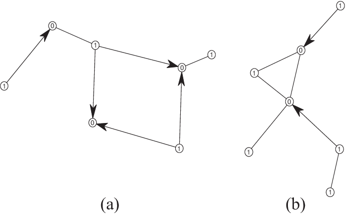
Figures 2 and 4 show examples of graph generated using this model.

We focus in the most challenging cases by selecting the number $D$ of available colors equal to the minimum feasible value $\chi(G)$.

Theorems 1 and 2 place connectivity requirements on the induced sensing graph $G^{\prime}$ in order to ensure that Algorithm 1 converges to a satisfying assignment. We begin by evaluating the fraction of random graphs in the Directed Boolean Model that meet these requirements. Figure 3 plots this fraction for a range of detection thresholds $R$ and vertex densities $\lambda$. It can be seen that for detection thresholds below $-15$ dBm greater than 96% of graphs satisfy the connectivity requirements. Figure 4 shows some examples of some DBM graphs corresponding to a $-25$ dBm threshold. Observe that they consist of a number of connected components and so the relaxed connectivity conditions provided by Theorems 2 are of considerable importance here. Note also that modern wireless devices typically have a noise floor of less than $-70$ dBm and so $-25$ dBm is conservative.

Moreover, Figure 3 shows the measured fraction of vertices for which Algorithm 1 successfully found a satisfying assignment for a detection threshold of $-25$ dBm. It can be seen that greater than 99.9% of vertices are successfully colored by the algorithm. For $\lambda=0.5$ and detection threshold of $-15$ dBm, 0.04% of the vertices that does not fulfill the conditions of Theorem 2 are still correctly colored by Algorithm 1. This small gap can be explained with the fact that the conditions of Theorem 2 are sufficient, but not necessary for convergence: some topologies can lead to convergence for their particular structure or because of a fortunate initial condition (see Figure 4 for some examples).

Figure 5 shows the measured distribution of convergence time for Algorithm 1 versus the detection threshold used for sensing. For a threshold of $-25$ dBm, the mean convergence time is less than 2000 iterations. When the required threshold is increased to $-15$ dBm, the mean convergence time decreases to less than 1000 iterations. These measurements are for a link density of $\lambda=0.5$, corresponding to on average 50 wireless links in an area of $100m^{2}$. Recall that we selected the number $D$ of available colors equal to the minimum feasible $\chi(G)$, thereby focussing on the most challenging situations. For larger numbers of colors it can be verified that the convergence time decreases exponentially in the number of colors above $\chi(G)$.

The comparison of the bounds given by Theorem 1 with the case without sensing restrictions given by Corollary 2 suggests that sensing restrictions lead to an increase in the convergence time. This is indeed the case, as shown in Figure 6, where the convergence rate of Algorithm 1 is shown with and without sensing restrictions for DBM graphs with $\lambda=0.5$ and detection threshold of $-15$ dBm. However for DMB graphs it can be seen that this increase is small.

We also analyzed in Section 7.1 the impact of the number of available colors on the convergence time.

Algorithm 1 was observed to converge in less than 1000 iterations in all examples. Figure 9 shows the measured distribution of convergence time for Algorithm 1 versus the detection threshold used for sensing. For a threshold of $-45$ dBm, corresponding to the target requirement noted above, the mean convergence time is less than 34 iterations. In a prototype lab set-up we have shown that an update interval of less than 10 seconds is feasible on current 802.11 hardware. Thus the mean time to convergence is under 6 minutes, which is a reasonable time-frame for practical purposes. When the required threshold is increased to $-30$ dBm, the mean convergence time decreases to less than 6 iterations i. e. under 1 minute when each iteration takes 10 seconds.

To examine the impact of the number of available colors we compare, in Figures 9 and 10, the convergence time when the number of colors is equal to $\chi$ and $\chi+2$ respectively. For a detection threshold of $-60$ dBm, adding two colors reduces the mean convergence time of almost 10 times.

References

- [1] K. Duffy, C. Bordenave, and D. Leith, “Decentralized Constraint Satisfaction,” CoRR, vol. abs/1103.3240, 2011.
- [2] J. Barcelo, B. Bellalta, C. Cano, A. Sfairopoulou, M. Oliver, and K. Verma, “Towards a Collision-free WLAN: Dynamic Parameter Adjustment in CSMA/E2CA,” EURASIP Journal on Wireless Communications and Networking, 2011.
- [3] M. Fang, D. Malone, K. Duffy, and D. Leith, “Decentralised Learning MACs for Collision-free Access in WLANs,” Wireless Networks, pp. 1–16, 2010.
- [4] A. Checco, R. Razavi, D. Leith, and H. Claussen, “Self-Configuration of Scrambling Codes for WCDMA Small Cell Networks,” in IEEE 23rd International Symposium on Personal, Indoor and Mobile Radio Communications (PIMRC), Sydney, Australia, September 2012.
- [5] A. Raniwala and T. Chiueh, “Architecture and Algorithms for an IEEE 802.11-based Multi-channel Wireless Mesh Network,” in INFOCOM 2005. 24th Annual Joint Conference of the IEEE Computer and Communications Societies. Proceedings IEEE, vol. 3. IEEE, 2005, pp. 2223–2234.
- [6] A. Mishra, V. Shrivastava, D. Agrawal, S. Banerjee, and S. Ganguly, “Distributed Channel Management in Uncoordinated Wireless Environments,” in Proceedings of the 12th Annual International Conference on Mobile Computing and Networking. ACM, 2006, pp. 170–181.
- [7] A. Mishra, V. Brik, S. Banerjee, A. Srinivasan, and W. Arbaugh, “A Client-driven Approach for Channel Management in Wireless LANs,” in in INFOCOM 2007. 25th Conference on Computer Communications, vol. 6, 2006.
- [8] K. Leung and B. Kim, “Frequency Assignment for IEEE 802.11 Wireless Networks,” in Vehicular Technology Conference, 2003. VTC 2003-Fall. 2003 IEEE 58th, vol. 3. IEEE, 2003, pp. 1422–1426.
- [9] L. Narayanan, Handbook of Wireless Network and Mobile Computing. Wiley Series on Parallel and Distributed Computing, 2002, ch. Channel Assignment and Graph Multicoloring.
- [10] O. Dousse, “Percolation in Directed Random Geometric Graphs,” in Information Theory Proceedings (ISIT), 2012 IEEE International Symposium on. IEEE, 2012, pp. 601–605.
- [11] K. Kothapalli, M. Onus, C. Scheideler, and C. Schindelhauer, “Distributed Coloring in -bits,” in Proc. of IEEE International Parallel and Distributed Processing Symposium (IPDPS), 2006.
- [12] S. Hedetniemi, D. Jacobs, and P. Srimani, “Fault Tolerant Distributed Coloring Algorithms that Stabilize in Linear Time,” in Proceedings of the IPDPS-2002 Workshop on Advances in Parallel and Distributed Computational Models, 2002, pp. 1–5.
- [13] Ö. Johansson, “Simple Distributed -coloring of Graphs,” Information Processing Letters, vol. 70, no. 5, pp. 229–232, 1999.
- [14] B. Kauffmann, F. Baccelli, A. Chaintreau, V. Mhatre, K. Papagiannaki, and C. Diot, “Measurement-based Self Organization of Interfering 802.11 Wireless Access Networks,” in INFOCOM 2007. 26th IEEE International Conference on Computer Communications. IEEE. IEEE, 2007, pp. 1451–1459.
- [15] ——, “Self Organization of Interfering 802.11 Wireless Access Networks,” in INFOCOM 2007. 26th IEEE International Conference on Computer Communications. IEEE, 2007.
- [16] P. Clifford and D. Leith, “Channel Dependent Interference and Decentralized Colouring,” Network Control and Optimization, pp. 95–104, 2007.
- [17] D. Leith, P. Clifford, V. Badarla, and D. Malone, “WLAN Channel Selection Without Communication,” Computer Networks, 2012.
- [18] G. Grimmett, Percolation. Springer, 1999, vol. 321.
- [19] “UE Radio transmission and Reception (FDD),” 3GPP TS25.101, Tech. Rep., 2004.
- [20] “wigle.net,” 2010. [Online]. Available: http://www.wigle.net/
- [21] IEEE Standard for Wireless LAN Medium Access Control (MAC) and Physical Layer (PHY) Specifications , Nov. 1997. P802.11, Std., 1997.
- [22] A. Goldsmith, Wireless Communications. Cambridge University Press, 2005.