IRFU-12-174
WUB/12-22
January, 2 2013
From hard exclusive meson electroproduction to deeply virtual Compton scattering
P. Kroll 11 1 Email: kroll@physik.uni-wuppertal.de
Fachbereich Physik, Universität Wuppertal, D-42097 Wuppertal,
Germany
and
Institut für Theoretische Physik, Universität
Regensburg,
D-93040 Regensburg, Germany
H. Moutarde 22 2 Email: herve.moutarde@cea.fr, F. Sabatié 33 3 Email: franck.sabatie@cea.fr
IRFU/Service de Physique Nucléaire, CEA Saclay, F-91191 Gif-sur-Yvette, France
Abstract
We systematically evaluate observables for hard exclusive electroproduction of real photons and compare them to experiment using a set of Generalized Parton Distributions (GPDs) whose parameters are constrained by Deeply Virtual Meson Production data, nucleon form factors and parton distributions. The Deeply Virtual Compton Scattering amplitudes are calculated to leading-twist accuracy and leading order in QCD perturbation theory while the leptonic tensor is treated exactly, without any approximation. This study constitutes a check of the universality of the GPDs. We summarize all relevant details on the parametrizations of the GPDs and describe its use in the handbag approach of the aforementioned hard scattering processes. We observe a good agreement between predictions and measurements of deeply virtual Compton scattering on a wide kinematic range, including most data from H1, ZEUS, HERMES, Hall A and CLAS collaborations for unpolarized and polarized targets when available. We also give predictions relevant for future experiments at COMPASS and JLab after the 12 GeV upgrade.
1 Introduction
For the last 15 years, the handbag approach to hard exclusive leptoproduction of photons (DVCS)44 4 Formally, Deeply Virtual Compton Scattering or DVCS refers only to the sub-process . However, DVCS is often used more loosely in the literature to name the photon leptoproduction process used experimentally. and mesons (DVMP) off protons has been extensively investigated both theoretically and experimentally. The handbag approach bases on factorization into hard (short-distance) partonic subprocesses and soft (long-distance) hadronic matrix elements [1, 2, 3, 4]. The latter are parametrized in terms of Generalized Parton Distributions (GPDs) [2, 5, 6]. The GPDs encode information on the longitudinal momentum distributions of the partons inside the proton as well as on the transverse localization of the partons [7, 8, 9]. The forward limits of some of the GPDs are the usual parton distributions (PDFs) and the lowest moments of the quark GPDs are related to the form factors of the proton. The GPDs give access to the total angular momenta of the partons making up the proton via Ji’s sum rule [2]. Another important property of the GPDs is their universality, i.e. the same GPDs occur in DVCS as well as in DVMP although in different flavor combinations. At present analytic methods to compute GPDs from QCD are lacking. Only lattice QCD provides numerical results on the lowest few moments of and quark GPDs [10, 11] for unphysical pion masses. There are also a number of models for GPDs available (e.g. Refs. [12, 13, 14, 15]) which can be confronted to experimental data on hard exclusive reactions in order to learn about GPDs.
In the late nineties when the phenomenology of hard exclusive reactions commenced, estimates of observables for such reactions were made on the basis of simple ansaetze for the GPDs, see for instance Refs. [16]–[22]. As it turned out in the course of time, these GPD models were insufficient to account for the increasing amount of accurate data coming from HERMES and Jefferson Lab. More complex parametrizations of the GPDs were invented and utilized to analyze independently the data on DVCS [23, 24] as well as DVMP for light vector mesons [25, 26] and for pions [27, 28]. It should be noted that in DVCS frequently only reduced amplitudes, the so-called Compton Form Factors (CFF), have been extracted [29, 30] which represent valuable constraints on the GPDs.
It is only recently that the universality property of GPDs has fully been exploited and a combined analysis of DVCS and DVMP carried through or a set of GPDs extracted from either DVCS or DVMP used to evaluate the other reaction. Thus, for instance, Meškaukas and Müller [31] performed a combined analysis of the HERA data on DVCS and DVMP. These authors also used the GPD advocated for in Refs. [25, 26] from an analysis of DVMP data, to compute DVCS observables for HERA kinematics. For a first attempt to compute DVCS along the same lines also for other kinematical regions see Müller et al in Ref. [32]. The results look quite promising, no severe discrepancy has been observed by these authors. In the present article we are going to study systematically predictions for DVCS in an leading-order (LO), lowest-twist calculation of the DVCS amplitudes using GPDs determined in Refs. [25, 26, 28]. In contrast to earlier work, e.g. Ref. [21], the leptonic tensor is evaluated without any approximation as it is done in Ref. [33] implying the inclusion of effects that are suppressed by powers of in our analysis. The primary goal of our study is to examine how realistic the considered set of GPDs is in order to eventually improve it if necessary.
The plan of the paper is as follows: in Sect. 2 we recapitulate the parametrization of the GPDs under scrutiny, and the theoretical description of the DVMP and DVCS processes in the handbag approach. In the second part, Sect. 3, we systematically compare model expectations to existing DVCS measurements. In Sect. 4 we give some predictions for observables which will be measured by the COMPASS, CLAS and Hall A collaborations in the near future. Finally, our summary and an outlook are presented in Sect. 5.
2 Theoretical description
2.1 The parametrization of the GPDs
In this section we recapitulate the parametrization of the GPDs used in Refs. [25, 26, 28] and specify all the ingredients required to fit the DVMP data. The GPDs are functions of three variables, the usual invariant momentum transfer, , the skewness defined as the ratio of light-cone plus components of the incoming () and outgoing () proton momenta
| (1) |
In the generalized Bjorken regime of large , large but fixed , it is related to Bjorken-, by :
| (2) |
where is the momentum of the virtual photon and its virtuality. The generalized Bjorken regime is defined by large and large photon-proton cms energy , but fixed . The third variable, , represents the average momentum fraction the emitted () and reabsorbed () partons carry with respect to the average proton momenta
| (3) |
GPDs further depend on a factorization scale [5], which is usually taken as the photon virtuality unless specified otherwise. At LO, leading-twist accuracy, only the GPDs contribute to DVCS which are characterized by the fact that the emitted and reabsorbed partons possess the same helicity. In Refs. [25, 26, 28] an integral representation of the GPDs is used
| (4) |
where is a double distribution [5, 34]55 5 The variables and are usually denoted by and , respectively. However, we do not use this notation here in order to avoid a clash of notation. These latter symbols are already used for powers in the functional form. and is the so-called -term [35] which appears for the gluon and flavor-singlet quark combination of the GPDs and . The label refers to specific quark flavors (or appropriate combinations) or to gluons. The -terms only contribute to the real parts of the amplitudes. At small skewness however, the amplitude is dominated by the imaginary part. In Refs. [25, 26, 28] the -terms are neglected. The advantage of the double-distribution ansatz for the GPDs is that polynomiality of the GPDs is automatically satisfied. For the GPDs and the -term ensures the appearance of the highest power of the skewness in the Mellin moments of the GPDs.
It is popular to write a double distribution as a product of a zero-skewness GPD and a weight function [34]
| (5) |
that generates the dependence of the GPD :
| (6) |
In Refs. [25, 26, 28] the parameter is taken as 1 for valence quarks and as 2 for sea quarks and gluons. The zero-skewness GPD is parametrized as the forward limit of that GPDs multiplied by an exponential in
| (7) |
The profile function, , is parametrized in a Regge-like manner
| (8) |
where represents the slope of an appropriate Regge trajectory and parametrizes the dependence of its residue. In Ref. [36] a more complicated profile function for valence quarks has been proposed
| (9) |
and exploited in an analysis of nucleon form factors. At small the Regge-like part dominates while, for , the term takes the lead. It turned out that there is a correlation between and : The small (large) behavior of the profile function controls the nucleon form factors at small (large) . For parametrizations like (7) without nodes except at the end-points, this correlation also holds for other moments of the GPDs and even for convolutions with hard scattering amplitudes. Thus, the Regge-like profile function is a sufficiently accurate approximation at small , the region we are interested in. It has also been shown in Refs. [37, 36] that, at large the Regge-like profile function leads to an unphysically large distance between the struck parton and the cluster of the spectators. This distance provides an estimate of the size of the proton as a whole.
The decomposition of the quark double distribution for the flavors and into and is done following the convention defined in Ref. [38] :
| (10) |
where for and and for and . For and and this prescription corresponds to the usual decomposition of parton distributions into valence quark and sea quark distributions, e.g. . The GPDs respect the symmetry relations
| (11) |
and
| (12) |
For DVCS the C-parity even combination of the double distributions is required
| (13) |
The parameters appearing in the double distributions, in particular in Eq. (7) and Eq. (8), are fixed in an analysis of DVMP data in the kinematical region specified by , , and . Cross section data are the only measurements available on a large range (up to about ) and they are dominated by contributions from the GPD . Other GPDs significantly enter asymmetries which are only measured for . Therefore evolution effects in this study are only sizeable for the GPD and can safely be neglected for other GPDs [26, 28]. Since the scale dependence of is available in [26], we still make use of it in our analysis of DVCS although it has practically no bearing on our results. It should be mentioned that in [25, 26] the evolution of the GPDs and is treated in an approximate way through the evolution of the PDFs in (7). A possible evolution of the profile function is ignored. At least for small skewness and small this approximation is reasonable as has been demonstrated in [26]. We follow this recipe which in any case is only of importance for the description of the DVCS cross section at HERA energies. It has been checked in Refs. [26, 28] that the valence quark GPDs are in agreement with the nucleon form factors at small and that all GPDs respect various positivity bounds [36, 39, 40]. At small there is also reasonable agreement between the moments of these GPDs and recent lattice results [10, 11]. But the GPD moments from lattice QCD have a flatter dependence than those obtained from the GPDs we are discussing here and also flatter than nucleon form factor data exhibit. A possible explanation comes from the unphysical values of the pion mass used in present lattice simulations and the contamination from excited states [41]. Chiral extrapolations of the lattice moments have not yet been systematically performed, see for instance Ref. [42].
2.1.1 Parametrization of the GPD
The GPD is rather well determined since it controls the cross sections for electroproduction of vector mesons for which a wealth of data is available. An advantage is that its forward limit occurring in Eq. (7), is a usual PDF. Therefore, only the parameters appearing in the profile functions have to be fixed. Linear Regge trajectories are assumed
| (14) |
As it is well-known the intercept controls the low- behavior of the PDF [43]. A standard Regge trajectory is assumed for the valence quarks, see Tab. 1. Since the sea-quark PDF is mainly driven by evolution for it is furthermore assumed that . The gluon trajectory with an effective scale-dependent intercept , is directly seen in the HERA experiments [44, 45] (and references therein) and consequently fixed by these data. This trajectory is also quoted in Tab. 1. The trajectories are accompanied by Regge residues assumed to have an exponential dependence, see Eq. (8), with slopes taken as ( being the proton mass)
| (15) |
It is convenient to expand the forward limits of , the PDFs, in a power series of (for ):
| (16) |
where, with regard to the fact that the forward limit of is defined as ,
| (17) |
The expansion coefficients have been obtained from a fit to the CTEQ6M PDFs [46]; they are compiled in Tab. 1 too.
The advantage of this expansion is twofold. First the integral (4) can be worked out term by term analytically leading to a corresponding expansion of the GPDs
| (18) |
The integrals are given explicitly in Ref. [26]. Second, the term in Eq. (16) guarantees that the longitudinal cross section on and electroproduction which is given by
| (19) |
at fixed and small (), is in reasonable agreement with the HERA data [44, 45]. The data used in current PDF analyses, for instance Refs. [47, 48] or more recent ones [49, 50, 51], do not constrain the gluon PDF well for . However, forcing the expansion of the gluon and sea PDFs to behave as at low always leads to reasonable agreement of the DVMP cross section with the HERA experiments. With this prescription other sets of PDFs, e.g. Refs. [47, 48], provide similar results as CTEQ6M. We stress that in all cases the expansions (16) are in good agreement with the original PDFs within their quoted errors.
Finally, in accord with CTEQ6 analysis, the quark sea is simplified in Ref. [26] as
| (20) |
where the dependence of the flavor symmetry breaking factor was taken from the CTEQ6M PDFs.
| gluon | strange | |||
| 0.48 | 0.48 | |||
| GeV-2 | 0.15 GeV-2 | 0.9 GeV-2 | 0.9 GeV-2 | |
| 0 | 0 |
2.1.2 Parametrization of
Much less is known about than for . There is only the analysis of the Pauli form factor [36] which provides information on for valence quarks. In addition there is an admittedly weak constraint from the asymmetries in electroproduction of mesons measured with a transversely polarized target [52, 53], for details see Sect. 2.2.
The GPD does not reduce to a PDF, the forward limit is not accessible in DIS. Therefore, the forward limit is to be fixed from exclusive experimental data as well. It is parametrized like the usual PDFs:
| (21) |
where is Euler’s beta function. The prefactor ensures the correct normalization of the Pauli form factor at . Indeed the moment
| (22) |
reduces to which is the flavor- contribution to the nucleon anomalous magnetic moment ( , ). The fits to the nucleon Pauli form factors performed in Ref. [36] fix the parameters specifying for valence quarks:
| (23) |
In the spirit of the Regge model, the trajectory is taken to be the same as in , see Tab. 1. The profile function (8) is evaluated with and with slope parameters taken to be zero.
All this specifies the double distribution (6) for . The GPDs are then obtained from Eq. (4) where the factor is expanded in a power series up to order 8 in order to perform the integration analytically. We stress that in the form factor analysis [36] the more complicated profile function (9) has been used while in the analysis of meson electroproduction [25, 26, 28] the small- approximation (8) is adopted. There is an ongoing reanalysis of the form factor data [54]; preliminary results are close to those of Eq. (23). The uncertainties in the determination of is reduced as compared to the results provided in Ref. [36].
The determination of for gluons and sea quarks is still in its infancy. A rough estimate of these GPDs has been made in Ref. [55] along the lines proposed by Diehl and Kugler [56]. Again the double distribution construction is used and the forward limits of the gluonic and strange quark GPDs are parametrized as
| (24) |
Of course the same Regge trajectory as for is used, see Tab. 1 and Eq. (17). The lack of detailed information forces the assumption of a flavor-symmetric sea. The powers of the large behavior are set to the following values (variant 3 of Tab. 1 in Ref. [55]):
| (25) |
The integer powers allow to solve the integral (4) analytically. The slope of the residues are taken as :
| (26) |
see Eq. (15). In Ref. [55] the normalization, , of is fixed from saturating a positivity bound [36] for a certain range of . Since the bound is quadratic the sign of is not fixed. Therefore, we have to consider the two cases .
The normalization of is fixed by using a sum rule for the second moments of [56]
| (27) |
The valence quark contribution to this sum rule is very small. Hence, the gluon and sea quark moments almost cancel each other. In any case, the sum rules allows to fix the normalization for given .
2.1.3 The GPD
The forward limit of reduces to the polarized PDF for which in Refs. [26, 28] the Blümlein-Böttcher results [57] are taken. To fix the parameters of only the HERMES data on the cross sections and the target asymmetries for electroproduction [58, 59] are at disposal. Therefore, is determined only for the valence quarks, and are neglected.
Analogously to Eq. (16) is expanded in a power series
| (28) |
where and is a normalization factor. The GPDs are constrained by the lowest moments at
| (29) |
which are known from and values and -decay constants in flavor SU(3)
| (30) |
This normalization is guaranteed by the factor
| (31) |
The expansion coefficients are compiled in Tab. 2 as well as the other parameters specifying this GPD.
| 0.48 | 0.48 | |
| 0.45 GeV-2 | 0.45 GeV-2 | |
| 0 | 0 | |
| 0.170+0.03 L | -0.320-0.040 L | |
| 1.340-0.02 L | -1.427-0.176 L | |
| 0.120-0.40 L | 0.692-0.068 L |
2.1.4 The GPD
Only exclusive electroproduction data constrain this GPD in the DVMP analysis. Therefore, as for , it can only be fixed for valence quarks. As is well-known it consists of two parts the pion-pole contribution and a non-pole one. The pole contribution reads [60, 61]
| (32) |
where is the pseudoscalar from factor of the nucleon. With the help of PCAC and the Goldberger-Treiman relation the pole contribution to the pseudoscalar form factor can be written as
| (33) |
Here () is the mass of the nucleon (pion), () is the pion-nucleon coupling constant, is the pion decay constant and is the pion’s distribution amplitude taken as:
| (34) |
The Gegenbauer coefficient is taken as at the initial scale . This value for is conform with the sharp rise of the transition form factor with as is observed by the Babar collaboration [62]. However, this behavior of the transition from factor is not seen by the BELLE collaboration [63]. The BELLE data are compatible with a pion distribution amplitude close to the asymptotic form . Since plays a minor role in DVCS we keep the value 0.22 for ; it practically has no bearing on our predictions for DVCS.
Finally, is the form factor of the pion-nucleon vertex and is parametrized in Ref. [28] as
| (35) |
with .
The non-pole contribution for which there is only a weak evidence in the data, is parameterized in the same spirit as the other GPDs. The forward limit is parametrized as in Refs. [28, 64]
| (36) |
Flavor independence of the Regge trajectory and the slope of its residue is assumed. The parameters for are compiled in Tab. 3.
| () | ||||
|---|---|---|---|---|
| 0.48 | 0.45 | 0.9 | 14.0 | 4.0 |
2.2 Description of DVMP
The particular variant of the handbag approach used to extract GPDs from meson electroproduction in the kinematical region of large and large but small and small invariant momentum transfer , is described in some detail in [25, 26]. Here, only the basic facts are reviewed. As an example, let us examine the helicity amplitudes for the asymptotically leading transitions from longitudinally polarized photons to likewise polarized mesons, :
| (37) |
within the handbag approach. The helicities of the protons are labeled by their signs and denotes the charge of the quark with flavor in units of the positron charge . To the proton helicity-non-flip amplitude the GPDs contribute in the combination
| (38) |
The terms in Eq. (37) denote convolutions of subprocess amplitudes and GPDs ():
| (39) |
where , and . The subprocess amplitude for partonic helicity is to be calculated perturbatively. Since is of the same order as in absolute value (see the discussion in Sec. 2.1), one can approximate by in the small skewness region. Moreover, for small the helicity-flip amplitude can also be neglected in the cross sections for vector mesons ( an exception is production) which is therefore only sensitive to .
As is well-known, in collinear factorization the handbag result for the integrated cross section scales as at fixed . However, for the kinematics accessible to current experiments, the data are in conflict with this prediction. This can be seen from Fig. 1 – the recent H1 data [44] on production only drop as . The theoretical behavior of the cross section is modified by logs of generated by the evolution of the GPDs; they diminish the discrepancy between theory and experiment. Experiment also tells us that the transverse cross section, , is not small; the ratio , also shown in Fig. 1, is rather small for experimentally accessible values of . Combining the data on the ratio with the unseparated cross section it becomes clear that the longitudinal cross section approximately falls off as too. This fact implies a marked overestimate of the longitudinal cross section at in the collinear approximation if it is evaluated from GPDs of the type discussed in Sect. 2.1.1. Agreement with experiment is however achieved in collinear approximation for an alternative parameterization of the GPD proposed in Ref. [31]. The evolution of this GPD produces much larger logs of than the GPD described in this article.


In view of this situation, power corrections are added to the LO subprocess amplitudes in Refs. [25, 26]. These power corrections are calculated within the modified perturbative approach [65] in which quark transverse degrees of freedom are kept and gluon radiation is taken into account. The latter has been calculated in the form of a Sudakov factor to next-to-leading-log approximation using resummation techniques and having recourse to the renormalization group [65]. For consistency, allowance is to be made for meson light-cone wave functions instead of distribution amplitudes. Due to these power corrections the convolutions also depend on . The modified perturbative approach is designed in such a way that asymptotically the collinear result for the subprocess amplitudes emerges. It is to be stressed that, in contrast to the situation at the mesonic vertex, the partons entering the subprocess are treated as being emitted and reabsorbed by the proton collinearly.
The above described approach can also be applied to vector mesons other than the and can be generalized to the asymptotically suppressed amplitudes for transitions66 6 Another method to treat transitions has been proposed in Ref. [66]. In collinear approximation these amplitudes are infrared singular but in the modified perturbative approach in the propagators regularizes the singular integrals. It should be mentioned that the described approach bears similarities to the color dipole model, see Ref. [67] and references therein. The described approach can also be applied to electroproduction of pseudoscalar mesons [28, 64] where one learns about the valence-quark components of GPDs and (see Sections 2.1.3 and 2.1.4) as well as on some of the transversity GPDs. However, the latter do not contribute to DVCS.

The available data from HERMES, COMPASS, E665, H1 and ZEUS on cross sections and spin density matrix elements for and electroproduction have been analyzed in Refs. [25, 26]. The data cover a large range of kinematics: varies between 3 and and between 5 and . In Fig. 1 the ratio is shown for electroproduction in order to demonstrate that a fair description of the amplitude for is also achieved. In Fig. 2 the longitudinal cross section for production is shown versus at . As the inspection of the figure reveals, a good description of all the low- data has been achieved for . For smaller the handbag results deviate from experiment; at theory and experiment deviate by orders of magnitude. For production, on the other hand, the handbag seems to work even at . More results and references to the experimental data can be found in Refs. [26, 68]. The HERMES cross section data on electroproduction data [58] as well as various single spin asymmetries are analyzed in Refs. [28, 64].
In the mentioned kinematical region, information on the GPD can only be extracted from the target asymmetry
| (40) |
which is obtained through the harmonic of the electroproduction asymmetry measured with a transversally polarized target. Here, is the azimuthal angle between the lepton and the hadron planes and specifies the orientation of the target spin vector with respect to the lepton plane (in the Trento convention [69]). The convolutions and in Eq. (40) are defined in Eq. (39). It is shown in Ref. [55] that the GPD described in Sect. 2.1.2 in combination with the rather well-known GPD , provides results in agreement with recent data on this asymmetry from the HERMES [52] and COMPASS [53] collaborations. It is to be stressed that for production the harmonic of the cross section for a transversally polarized target essentially probes for valence quarks; the gluon and sea-quark contributions cancel each other to a large extent due to the sum rule (27) which implies that the second moments of and have about the same strength but opposite sign. For the simple parametrization (24) with no nodes except at the end-points, this property of the second moments transfers to other moments of to a certain degree and in particular to the convolutions. In accord with this argument, for electroproduction of the mesons is predicted to be about zero in agreement with preliminary HERMES data [70].
2.3 DVCS in the handbag approach
In the following we use the aforementioned GPDs constrained from DVMP, nucleon form factors and partons distributions to evaluate observables and compare to measurements. As for DVMP we will analyze this process in the generalized Bjorken regime of large , large but fixed .
Leptoproduction of photons is complicated since, besides the DVCS contribution, , there is also the Bethe-Heitler (BH) contribution. The square of the amplitude therefore falls into three parts :
| (41) |
These parts readily correspond to the squared amplitudes of the BH and DVCS processes and their interference. In the one-photon-exchange approximation of QED, the three terms , and in (41) have the following harmonic structure in , the azimuthal angle of the outgoing photon with regard to the leptonic plane (in the Trento convention [69]) :
| (42) |
where comes from the BH lepton propagators. Although there are only harmonics up to the maximal order 3 in the sums, the additional dependence from the lepton propagators generates in principle an infinite series of harmonics for the BH and interference terms. A more detailed harmonic structure taking into account beam and target polarizations, can be found for instance in [71]. For transverse target polarization the harmonic series also depends on the angle which specifies the orientation of the target spin vector. An harmonic analysis of allows for an examination of the GPDs [72]. Detailed analytic expressions describing this harmonic structure were published in Ref. [21]. They involve CFFs, which are integrals of GPDs over the momentum fraction with a hard scattering kernel. At LO the CFFs read :
| (43) |
where is defined after Eq. (10). The CFFs, the analogues of the convolutions (39) for DVMP, are complex functions due to the singularity at in the integration domain.
In Ref. [21] the electroproduction of photons was evaluated to leading and subleading order in an expansion. Since a great wealth of data in the valence region [73, 74] involve not-so-large values of , the impact of this approximation is not negligible when comparing theoretical expectations and measurements. In 2008 Guichon and Vanderhaeghen [75] elaborated on their previous numerical computations [60, 76, 77] of the process to establish analytic expressions of the cross section for all polarizations of the proton target and of the incoming lepton. In these formulas the leptonic tensor is treated exactly, i.e. the involved kinematic terms are kept with their full dependence : they are not expanded as power in . These analytic expressions were implemented into a ROOT/C++ code [30] and it was checked in Ref. [78] that they are completely equivalent to the expressions of cross sections for all polarizations of the proton target and of the incoming lepton, presented in Refs. [60, 76, 77]. Later Belitsky and Mueller extended their earlier work [21] by removing the approximations done in the expansion of the leptonic tensor [79, 33]. Note that the case of the transverse target polarization is not treated in these references.
In the present work, we use the theoretical framework of Guichon and Vanderhaeghen which provides a complete and accurate set of formulas that encompass all types of polarizations, including the case of a transverse target. Our approach is consistent with the so-called BM formalism [33].
Further improvements of this approach have been considered: the next-to-leading order (NLO) kernels have been calculated in Refs. [80, 81, 82, 83, 84]. Soft-collinear resummation formulas have been derived recently [85]. Finite- and target-mass corrections to DVCS have recently been investigated in the OPE framework in Refs. [86, 87] (and references therein). Twist-3 effects in DVCS have also been studied in Refs. [88, 89, 90]. The phenomenological implications of all these corrections for DVCS observables remain to be studied. This is beyond the scope of the present article.
3 Comparison to DVCS data
The cross section on an unpolarized target for a given beam charge, in units of the positron charge and beam helicity can be written as :
| (44) |
where only the dependence of the observables is shown. If both longitudinally polarized positively and negatively charged beams are available, the asymmetries in Eq. (44) can be isolated, as is the case for a large part of HERMES data. Thus, for instance the beam charge asymmetry is obtained from the combination :
| (45) |
From analogous combinations, one obtains the two beam spin asymmetries and :
| (46) | |||||
| (47) |
If an experiment only has access to one value of such as in Jefferson Lab, the asymmetries defined in Eq. (44) cannot be isolated and one can only measure the beam spin asymmetry which depends on the charge-spin cross section as follows :
| (48) |
where we use the familiar notation of labeling the charge-spin cross section by the sign of the beam charge and an arrow () for the helicity plus (minus). One can check that can be written as a function of the spin and charge asymmetries defined in Eq. (44) :
| (49) |
The case of longitudinally polarized target observables is simpler, due to the fact that there are no data with both varying longitudinal target polarization and beam charge. Therefore, experiments measured the target longitudinal spin asymmetry which reads :
| (50) |
where the double arrows () refer to the target polarization state parallel (anti-parallel) to the beam momentum. The double longitudinal target spin asymmetry is defined in a similar fashion :
| (51) |
The HERMES collaboration also had access to a transversally polarized target with both electrons and positrons. They therefore were able to measure two types of observables :
| (52) | |||||
| (53) | |||||
Finally, it is worth mentioning that the HERMES collaboration usually does not publish the -dependence of the asymmetries but rather chose to extract harmonics out of their asymmetries. For instance, in the case of the beam charge asymmetry , the harmonics are extracted using the following formula :
| (54) |
where the normalization factor is in the case and for . Since HERMES has not measured numerators () and denominators () of the asymmetries in Eqs. (45) - (53) separately the projection (54) is the best approximation to the Fourier coefficients
| (55) |
HERMES can do. The latter Fourier coefficients are closest related to the CFFs.
The coefficients of the various Fourier harmonics occurring in Eq. (42) provide information about CFFs, or equivalently GPDs, either in the interference with the real Bethe-Heitler amplitude or from the DVCS process. Through the measurement of cross sections or the various asymmetries described in Eqs. (45)–(53), one can put constraints on different combination of GPDs. As an illustration we quote the leading-twist, LO pQCD connection between observables and CFF for some asymmetries [21, 33, 71] :
| (56) | |||||
| Experiment | Observable | Normalized CFF dependence |
|---|---|---|
| HERMES | ||
| CLAS | ||
| HALL A | ||
| HERA |
| Kinematics | |||
|---|---|---|---|
| Experiment | [GeV2] | [GeV2] | |
| HERMES | 0.09 | 2.50 | -0.12 |
| CLAS | 0.19 | 1.25 | -0.19 |
| HALL A | 0.36 | 2.30 | -0.23 |
| HERA | 0.001 | 8.00 | -0.30 |
In the following subsections, we compare predictions on DVCS evaluated from the GPDs described in Sect. 2.1 to the available data in different kinematic domains : from small (H1, ZEUS) [91]–[94] to intermediate (HERMES) [95]–[98] and large (Jefferson Lab Hall A and CLAS) [73, 74, 99]. The HERA H1 and ZEUS collaborations measured the DVCS () cross section at large and but small , which are mostly sensitive to the imaginary part of . HERMES measured and published a large number of asymmetries with different beam charge, helicity states and target polarization. These data lie in the range and are sensitive to the real and imaginary parts of the CFFs , and . The data sets from Jefferson Lab either cover a wide kinematic range () [74] or are highly precise on a restricted kinematic domain [73]. In the first case beam spin asymmetries are measured, and in the second helicity-dependent and independent cross sections. The dependence of all these observables to the CFFs are compiled in Tab. 4 where for each experiment, we have chosen the typical kinematics listed in Tab. 5. The BH amplitude is evaluated from the Kelly parametrization of nucleon form factors [100]. We would like to stress once again that no DVCS data has been used in order to fix the GPD parameters. Observables which vanish to the accuracy we are working and for which the data are compatible with zero within errors will not be discussed in the following. The propagation of PDF errors to the GPDs and is the only source of uncertainties we have considered so far. They will be shown as shadowed bands around the predictions on all the following figures.
3.1 Beam charge asymmetry
We begin the discussion with the beam charge asymmetry, , as measured by the HERMES collaboration during 1996–2007, a result which has been recently updated in Ref. [97]. This observable is generated by the BH-DVCS interference term (see Eq. (56)) which, to leading-twist accuracy, feeds the harmonics (). As inspection of Tab. 4 reveals, both the harmonics depend mostly on the real part of the CFF . In Fig. 3, our predictions are compared to the HERMES data [97]. Very good agreement can be seen for both the harmonics, demonstrating that in this kinematical range, the real part of has the right magnitude.

3.2 Beam spin asymmetry
As can be seen from Eq. (56) the harmonic of the beam spin asymmetry, , depends on the same combination of electromagnetic form factors and CFFs as the beam charge asymmetry. As we already mentioned this combination is dominated by the GPD , see Tab. 4. Since the electromagnetic form factors are real, the imaginary part of the CFF is required which, to leading-order of perturbative QCD (see (43)), is given by the GPD at the cross-over line , i.e. essentially probes the combination
| (57) |
Our results for the beam spin asymmetry are shown in Fig. 4-left and compared to the HERMES data [97]. The agreement between predictions and data is not as good in this case, our results differ by about ( in absolute value) from experiment. Recently the HERMES collaboration has published data on the harmonic of the beam spin asymmetry using a recoil detector and a positron beam [98]. In this experiment all three final state particles are detected and therefore the resonant background severely reduced. In so far the recoil data are closer to the exclusive process to which our theory applies. The data were taken at about the same average values of and . In order to compare to recoil data, we computed using Eq. (49) with and from the non-recoil data and (exact at twist 2 and in agreement with experimental results from Ref. [97]). Then the coefficient is :
| (58) |
On the right hand side of Fig. 4 we therefore show both from the non-recoil and the recoil data. We observe that the recoil data are significantly larger in absolute value, yielding very good agreement with our predictions. Similar effects for other DVCS observables may occur but with the exception of the beam spin asymmetry, there are no measurements with the recoil detector available. The effect of the resonant background in other observables is unknown. Note that vanishes for forward scattering, . The trend towards zero is however only visible for of order which is very small, about for HERMES kinematics.

The CLAS collaboration published accurate data on the beam helicity asymmetry in a large kinematical range [74]. The data analysis required the detection of the full final state, much like the HERMES recoil data. A selected sample of the -dependent asymmetry is shown on Fig. 5. While the dominance of the term is clearly visible in the data one notices a discrepancy between the data and our prediction of the same order as for the non-recoil HERMES beam spin asymmetry, see above. We repeat - our GPDs are optimized for small skewness (see discussion in Sect. 2.1 and Sect. 2.2) and one therefore cannot expect perfect agreement with large-skewness experiment.

3.3 Longitudinal target polarization
This asymmetry is very similar to the beam spin asymmetry in that it is dominated by the DVCS-BH interference. The most important observable of this type is which is primarily sensitive to as an inspection of Tab. 4 reveals. The comparison of the HERMES data [96] on this observable measured with a positron beam, with our predictions is made in Fig. 6 and, given the large experimental errors, reasonable agreement is observed. Only at small our result seems slightly larger in absolute value than the data by a fraction of the HERMES error bar. A surprisingly large harmonic appears in the HERMES data, see Fig. 6. Theoretically this contribution should be heavily suppressed to the order we are working and indeed our prediction is very small. The reason for the large experimental value of is unclear. For both parameters the figure also shows the contribution from separately, confirming that this GPD represents a significant fraction of .

The CLAS collaboration has published data on [99], integrated over a large kinematical bin. In contrast to HERMES this collaboration uses an electron beam implying that the BH-DVCS interference contributes with opposite sign to than in the HERMES data on . The and harmonics are shown in Fig. 7 along with our predictions. In contrast to the HERMES data, the harmonic is compatible with zero, however our prediction is small and positive, off by about 1.5 . For the harmonic, our result and the CLAS data are in perfect agreement.

HERMES has also measured the double-spin asymmetry for a longitudinally polarized beam and target. In contrast to the single spin asymmetries and the BH term contributes to . In fact it provides the dominant contribution to the term and about half the magnitude of the harmonic, see Fig. 6. Thus, at the current experimental accuracy in these observables, no information about GPDs can be extracted. Our full results for are of course in agreement with HERMES data as can be seen from Fig. 6.
3.4 Transversely polarized target
The harmonic of the transverse target spin asymmetry is especially interesting since it is generated by the squared DVCS contribution and it is mostly sensitive to , see Eq. (56) and Tab. 4. For given it is uniquely sensitive to the CFF . It therefore constitutes one of the few ways to constrain the GPD . The valence part of is rather well constrained by fits to the data of the nucleon form factors [36] and is in fair agreement with the data on for electroproduction [52, 53]. As we discussed in Sect. 2.2 for production the contributions from for sea quarks and gluons cancel to a large extent. In view of this the DVCS data on are complementary to DVMP and especially important because to LO QCD there is no contribution from and therefore the cancellation between the gluon and sea-quark contributions cannot happen. Hence, for DVCS probes the sea-quark part of for given GPDs and . We remark that is forced to vanish for forward scattering by angular momentum conservation.
The HERMES data [95] on the harmonics of is shown in Fig. 8. Also shown in Fig. 8 is . This observable receives separate contributions from Im, Im and Im (see Eq. (56) and Tab. 4) and even for reasonable agreement with experiment is achieved. In contrast to this observable would vanish if was zero which is not the case experimentally.
In order to check the normalization of the GPD for a flavor symmetric sea we also display in Fig. 8 results for three different normalizations of : and ; for the latter value a positivity bound is saturated [55] (see Sect. 2.1.2). It can be seen from the figure that a negative seems to be favored. Considering the large errors of the data, a value of close to zero but negative is not excluded while a large positive value is apparently in conflict with experiment.

3.5 Hall A cross sections
The helicity-dependent cross section has been measured by the Hall A collaboration at Jefferson Lab [73] at fixed =0.36. These data are extremely accurate and are therefore very demanding to theory. They have the advantage to cleanly separate the difference of the cross sections for opposite electron helicities, , from their sum, . The main contribution to the cross section difference is the harmonic fed by the BH-DVCS interference. From Tab. 4 we see that the most prominent contribution from the CFFs is . The cross section sum, on the other hand, which corresponds to the unpolarized cross section, receives contributions from all three terms BH, DVCS and the BH-DVCS interference but the BH contribution is dominant. Its most prominent harmonics are and .

The comparison of the difference and sum of the Hall A helicity cross sections with our results at their highest bin is shown in Fig. 9. The agreement is nearly perfect for which indicates that our parameterization of seems to be adequate. This is in line with our findings for at HERMES kinematics, namely that our predictions agree well with the recoil data [98].
The cross section sum exhibits the expected dependence of a linear combination of the and harmonics. There is however a discrepancy between theory and experiment of up to 30% in the strength, especially around , pointing to something missing in the real parts of the various CFFs entering this observable, in particular , see Tab. 4. Note that by taking the ratio of the difference over the sum of cross-sections for Hall A, one recovers a result fully compatible with the CLAS beam spin asymmetry data in the same kinematical range. It is therefore no surprise that our approach also has difficulties reproducing the CLAS beam spin asymmetries since the issue apparently lies in the unpolarized cross section. The real part of is also probed by . Since contributes to with a small coefficient as compared to the BH-term, a substantial increase of would be required in order to fit the Hall A data. Whether such an increase is compatible with other DVCS and DVMP data remains to be seen. In any case, we would like to stress again that the GPD parametrization we are using has been tuned to much lower values of . Thus, for instance, the addition of a D-term to the double-distribution might improve the agreement between theory and experiment. The exploration of this as well as other improvements of the GPDs is left for future work.
3.6 H1 and ZEUS cross sections
The H1 [91, 92] and ZEUS [93, 94] collaborations published -differential cross section. The kinematics for these data is characterized by small , typically , a photon virtuality that varies between 3 and and large , of order . In this kinematical range the GPDs at small skewness and small control the DVCS cross section. The dominant contribution to the cross sections comes from the GPD . The GPD is suppressed, see Tab. 4. The contribution from , although not suppressed as compared to (see Tab. 4), is negligible here since is much smaller than ; this is in particular the case for the sea quark contribution. We remark that for the leptoproduction of vector mesons, does not contribute to leading-twist accuracy. Due to the large range of in which the HERA data are available, evolution of the GPD plays a decisive role. Using the scale-dependent parametrization of introduced in Sect. 2.1.1 we evaluate the DVCS cross section at HERA kinematics to leading-twist accuracy and LO of perturbative QCD. As the factorization scale we choose . Our results are compared to the HERA data in Fig. 10. Reasonable agreement with experiment is achieved within experimental errors and theoretical uncertainties. A similar observation has also been made in [31]. In this paper only the GPD is taken into account and parametrized in terms of an SO(3) -channel partial wave expansion. A combined fit of the GPD parameters to the HERA DVCS and DVMP data is performed. In contrast to the analysis carried through in [25, 26] (see Sect. 2.2) DVMP is also computed within the collinear factorization approach. This necessitates a GPD that differs from the one we are using in particular at the cross-over line , and that leads to very strong evolution effects. The quality of the combined fit to the HERA data on DVCS and DVMP performed in [31] is comparable to that of our results.

4 Future Experiments
The COMPASS collaboration will have a two-week DVCS run in 2012 with a 160 GeV muon beam, followed by a longer run in 2015 and later [101]. They plan to measure the -slope of the -integrated photon electroproduction cross section, as well as specific charge and spin observables. The polarized muon beam is produced through pion decay, its polarization therefore changes sign when the beam charge is reversed, i.e. and are polarized along opposite directions. COMPASS plans to measure mixed charge-spin (CS) cross sections differences and sums defined as follows:
| (59) |
where the cross sections are defined in Eq. (44). Predictions from our approach for these three observables are shown in Fig. 11 along with predictions made in Ref. [24].

The CLAS12 collaboration plans to measure the beam and target spin asymmetries as well as cross sections for DVCS with the 11 GeV electron beam as soon as 2015 [102]. In Fig. 12 our predictions for the moments of the beam and target spin asymmetries and , evaluated with the help of the analogue of (54), are displayed for a typical kinematical bin accessible with CLAS12. The Hall A collaboration will also run a DVCS experiment very soon after the 12 GeV upgrade is complete [103]. Our predictions for the difference and sum of the helicity cross sections are shown in Fig. 12 for one of the planned kinematical settings.
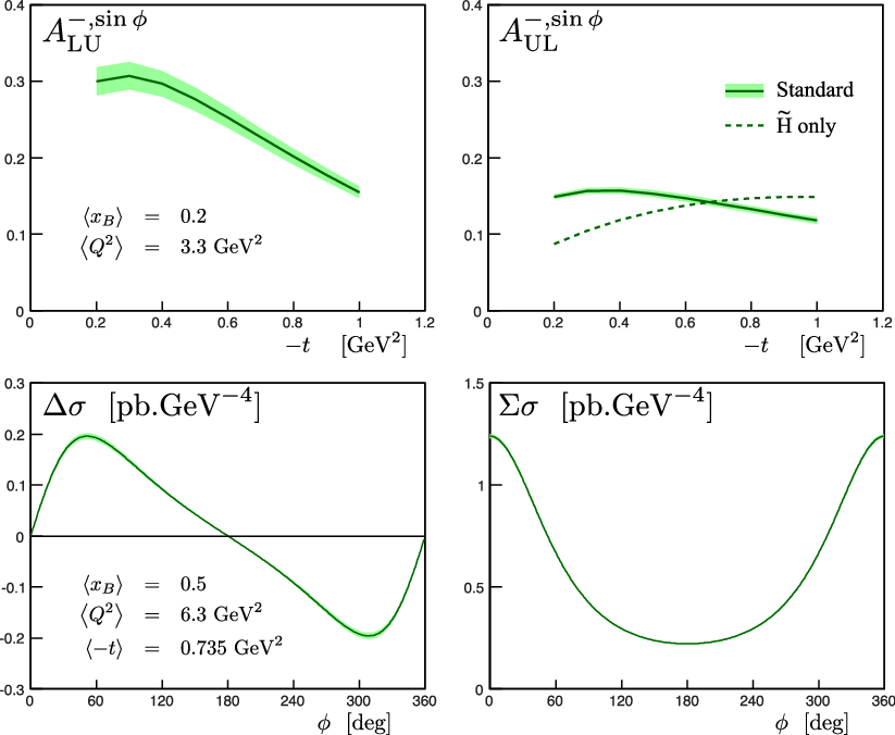
More detailed predictions can be obtained from the authors on request.
5 Summary and outlook
Since 2000 there has been a great wealth of measurements related to the DVMP and DVCS processes. Factorization theorems assert that these hard exclusive processes can be interpreted in terms of partonic degrees of freedom, provided the virtuality of the exchanged photon is large enough. In that case the partonic picture involves GPDs, which are universal, process-independent quantities. Up to now, both processes have mostly been studied independently of each other, and it is therefore an important check of consistency to test whether the GPDs used to describe one channel can be used to describe the other channel as well. Obviously universality is exploited at the most in a combined analysis of both DVMP and DVCS but this large-scale program is beyond the scope of the present article.
A necessary and interesting first step in exploiting universality is the use of a set of GPDs extracted from an analysis of DVMP data from H1, ZEUS, E665, COMPASS and HERMES [26, 28, 55] in a then parameter-free evaluation of DVCS and the detailed comparison with the available data. The various observables are computed within an approach in which the DVCS amplitudes are calculated to leading-twist accuracy and leading-order perturbative QCD while, similarly to Ref. [33], the leptonic tensor is taken into account without any approximation. We stress that DVCS is treated in the collinear factorization framework. This is consistent with the calculation of DVMP as described in Sect. 2.2 and hence, the GPDs extracted from DVMP can be used for the calculation of DVCS observables. In both processes the quarks are emitted and reabsorbed from the proton collinearly with the proton momenta.
We observe very good overall agreement between our predictions and most of the H1, ZEUS and HERMES data but a less satisfactory description of the large (small ) data from Jefferson Lab, where power corrections might be large. We notice that the most recent HERMES measurements [98] using a recoil detector in order to achieve fully exclusive final states, give a significantly larger beam spin asymmetry (in absolute value). The recoil data are in perfect agreement with our results. Such dilution effect may be present in other HERMES observables as well and estimates of this effect would be highly valuable. The COMPASS, CLAS12 and Hall A collaborations have planned to take DVCS data in the coming years. In view of the good agreement with the available data demonstrated in our study we also give predictions for their main observables.
Our study makes it clear that the set of GPDs we are using which is extracted from DVMP, describes DVCS data over a large kinematical range rather well in general although not perfectly in all details. This is partly a consequence of the different kinematic ranges of DVCS measurements and of the DVMP data used to constrain our GPD model. In addition, the GPD parametrization is of course an approximation. Thus, improvements of the GPD parametrization are required on the long run. In order to do so future data from COMPASS and JLab12 will be of help. Possible improvements may include the use of more recent versions of the PDFs, the proper scale dependence of the GPDs, an updated form factor analysis [54], eventual modifications of the profile functions of the double distribution parameterization and allowance for a non-zero -term.
Acknowledgments
The authors would like to thank M. Diehl, N. D’Hose, D. Müller, W.-D. Nowak and G. Schnell for many fruitful discussions and valuable inputs.
This work was supported in part by the Commissariat à l’Energie Atomique et aux Energies Alternatives and the GDR 3034 PH-QCD and by the BMBF under contract 06RY258.
References
- [1] A.V. Radyushkin, Phys. Lett. B 385, 333 (1996) [hep-ph/9605431].
- [2] X. -D. Ji, Phys. Rev. D 55, 7114 (1997) [hep-ph/9609381].
- [3] J.C. Collins, L. Frankfurt and M. Strikman, Phys. Rev. D 56, 2982 (1997) [hep-ph/9611433].
- [4] J. C. Collins and A. Freund, Phys. Rev. D 59, 074009 (1999) [hep-ph/9801262].
- [5] D. Mueller, D. Robaschik, B. Geyer, F. M. Dittes and J. Horejsi, Fortsch. Phys. 42, 101 (1994) [hep-ph/9812448].
- [6] A. V. Radyushkin, Phys. Rev. D 56, 5524 (1997) [hep-ph/9704207].
- [7] M. Burkardt, Phys. Rev. D 62, 071503 (2000) [Erratum-ibid. D 66, 119903 (2002)] [hep-ph/0005108].
- [8] M. Diehl, Eur. Phys. J. C 25, 223 (2002) [Erratum-ibid. C 31, 277 (2003)] [hep-ph/0205208].
- [9] J. P. Ralston and B. Pire, Phys. Rev. D 66, 111501 (2002) [hep-ph/0110075].
- [10] J. D. Bratt et al. [LHPC Collaboration], Phys. Rev. D 82, 094502 (2010) [arXiv:1001.3620 [hep-lat]].
- [11] S. Collins, M. Gockeler, P. Hagler, R. Horsley, Y. Nakamura, A. Nobile, D. Pleiter and P. E. L. Rakow et al., Phys. Rev. D 84, 074507 (2011) [arXiv:1106.3580 [hep-lat]].
- [12] V. Y. .Petrov, P. V. Pobylitsa, M. V. Polyakov, I. Bornig, K. Goeke and C. Weiss, Phys. Rev. D 57, 4325 (1998) [hep-ph/9710270].
- [13] M. Diehl, T. Feldmann, R. Jakob and P. Kroll, Eur. Phys. J. C 8, 409 (1999) [hep-ph/9811253].
- [14] S. Scopetta and V. Vento, Phys. Rev. D 71, 014014 (2005) [hep-ph/0410191].
- [15] C. Lorce and B. Pasquini, Phys. Rev. D 84, 014015 (2011) [arXiv:1106.0139 [hep-ph]].
- [16] L. Mankiewicz, G. Piller and T. Weigl, Phys. Rev. D 59, 017501 (1999) [hep-ph/9712508].
- [17] L. Mankiewicz, G. Piller and A. Radyushkin, Eur. Phys. J. C 10, 307 (1999) [hep-ph/9812467].
- [18] L. L. Frankfurt, P. V. Pobylitsa, M. V. Polyakov and M. Strikman, Phys. Rev. D 60, 014010 (1999) [hep-ph/9901429].
- [19] M. Vanderhaeghen, P. A. M. Guichon and M. Guidal, Phys. Rev. D 60, 094017 (1999) [hep-ph/9905372].
- [20] A. V. Belitsky, D. Mueller, L. Niedermeier and A. Schafer, Nucl. Phys. B 593, 289 (2001) [hep-ph/0004059].
- [21] A. V. Belitsky, D. Mueller and A. Kirchner, Nucl. Phys. B 629, 323 (2002) [hep-ph/0112108].
- [22] A. Freund and M. F. McDermott, Phys. Rev. D 65, 074008 (2002) [hep-ph/0106319].
- [23] K. Kumericki, D. Mueller and K. Passek-Kumericki, Nucl. Phys. B 794, 244 (2008) [hep-ph/0703179].
- [24] K. Kumericki and D. Mueller, Nucl. Phys. B 841, 1 (2010) [arXiv:0904.0458 [hep-ph]].
- [25] S. V. Goloskokov and P. Kroll, Eur. Phys. J. C 42, 281 (2005) [hep-ph/0501242].
- [26] S. V. Goloskokov and P. Kroll, Eur. Phys. J. C 53, 367 (2008) [arXiv:0708.3569 [hep-ph]].
- [27] S. Ahmad, G. R. Goldstein and S. Liuti, Phys. Rev. D 79, 054014 (2009) [arXiv:0805.3568 [hep-ph]].
- [28] S. V. Goloskokov and P. Kroll, Eur. Phys. J. C 65, 137 (2010) [arXiv:0906.0460 [hep-ph]].
- [29] M. Guidal and H. Moutarde, Eur. Phys. J. A 42, 71 (2009) [arXiv:0905.1220 [hep-ph]].
- [30] H. Moutarde, Phys. Rev. D 79, 094021 (2009) [arXiv:0904.1648 [hep-ph]].
- [31] M. Meskauskas and D. Mueller, [arXiv:1112.2597 [hep-ph]].
- [32] D. Boer, M. Diehl, R. Milner, R. Venugopalan, W. Vogelsang, D. Kaplan, H. Montgomery and S. Vigdor et al., [arXiv:1108.1713 [nucl-th]].
- [33] A.V. Belitsky and D. Mueller, Phys. Rev. D 82, 074010 (2010) [arXiv:1005.5209 [hep-ph]].
- [34] A. V. Radyushkin, Phys. Lett. B 449, 81 (1999) [hep-ph/9810466].
- [35] M. V. Polyakov and C. Weiss, Phys. Rev. D 60, 114017 (1999) [hep-ph/9902451].
- [36] M. Diehl, T. Feldmann, R. Jakob and P. Kroll, Eur. Phys. J. C 39, 1 (2005) [hep-ph/0408173].
- [37] M. Burkardt, Int. J. Mod. Phys. A 18, 173 (2003) [hep-ph/0207047].
- [38] M. Diehl, Phys. Rept. 388, 41 (2003) [hep-ph/0307382].
- [39] P. V. Pobylitsa, Phys. Rev. D 66, 094002 (2002) [hep-ph/0204337].
- [40] M. Burkardt, Phys. Lett. B 582, 151 (2004) [hep-ph/0309116].
- [41] J. R. Green, M. Engelhardt, S. Krieg, J. W. Negele, A. V. Pochinsky and S. N. Syritsyn, arXiv:1209.1687 [hep-lat].
- [42] G. S. Bali, S. Collins, M. Deka, B. Glaessle, M. Gockeler, J. Najjar, A. Nobile and D. Pleiter et al., Phys. Rev. D 86, 054504 (2012) [arXiv:1207.1110 [hep-lat]].
- [43] P. V. Landshoff, J. C. Polkinghorne and R. D. Short, Nucl. Phys. B 28, 225 (1971).
- [44] F. D. Aaron et al. [H1 Collaboration], JHEP 1005, 032 (2010) [arXiv:0910.5831 [hep-ex]].
- [45] S. Chekanov et al. [ZEUS Collaboration], PMC Phys. A 1, 6 (2007) [arXiv:0708.1478 [hep-ex]].
- [46] J. Pumplin, D. R. Stump, J. Huston, H. L. Lai, P. M. Nadolsky and W. K. Tung, JHEP 0207, 012 (2002) [hep-ph/0201195].
- [47] A. D. Martin, R. G. Roberts, W. J. Stirling and R. S. Thorne, Eur. Phys. J. C 23, 73 (2002) [hep-ph/0110215].
- [48] S. Alekhin, JETP Lett. 82, 628 (2005) [Pisma Zh. Eksp. Teor. Fiz. 82, 710 (2005)] [hep-ph/0508248].
- [49] H. -L. Lai, M. Guzzi, J. Huston, Z. Li, P. M. Nadolsky, J. Pumplin and C. -P. Yuan, Phys. Rev. D 82, 074024 (2010) [arXiv:1007.2241 [hep-ph]].
- [50] A. D. Martin, W. J. Stirling, R. S. Thorne and G. Watt, Eur. Phys. J. C 70, 51 (2010) [arXiv:1007.2624 [hep-ph]].
- [51] R. D. Ball et al. [NNPDF Collaboration], Nucl. Phys. B 809, 1 (2009) [Erratum-ibid. B 816, 293 (2009)] [arXiv:0808.1231 [hep-ph]].
- [52] A. Airapetian et al. [HERMES Collaboration], Phys. Lett. B 679, 100 (2009) [arXiv:0906.5160 [hep-ex]].
- [53] C. Adolph et al., [COMPASS Collaboration], Nucl. Phys. B 865, 1 (2012) [arXiv:1207.4301 [hep-ex]].
- [54] M. Diehl and P. Kroll, work in progress.
- [55] S. V. Goloskokov and P. Kroll, Eur. Phys. J. C 59, 809 (2009) [arXiv:0809.4126 [hep-ph]].
- [56] M. Diehl and W. Kugler, Eur. Phys. J. C 52, 933 (2007) [arXiv:0708.1121 [hep-ph]].
- [57] J. Blümlein and H. Böttcher, Nucl. Phys. B 636, 225 (2002) [hep-ph/0203155].
- [58] A. Airapetian et al. [HERMES Collaboration], Phys. Lett. B 659, 486 (2008) [arXiv:0707.0222 [hep-ex]].
- [59] A. Airapetian et al. [HERMES Collaboration], Phys. Lett. B 682, 345 (2010) [arXiv:0907.2596 [hep-ex]].
- [60] M. Vanderhaeghen, P. A. M. Guichon and M. Guidal, Phys. Rev. D 60, 094017 (1999) [hep-ph/9905372].
- [61] M. Penttinen, M. V. Polyakov and K. Goeke, Phys. Rev. D 62, 014024 (2000) [hep-ph/9909489].
- [62] B. Aubert et al. [BABAR Collaboration], Phys. Rev. D 80, 052002 (2009) [arXiv:0905.4778 [hep-ex]].
- [63] S. Uehara et al. [Belle Collaboration], [arXiv:1205.3249 [hep-ex]].
- [64] S. V. Goloskokov and P. Kroll, Eur. Phys. J. A 47, 112 (2011) [arXiv:1106.4897 [hep-ph]].
- [65] J. Botts and G. Sterman, Nucl. Phys. B 325, 62 (1989).
- [66] I. V. Anikin, D. Y. .Ivanov, B. Pire, L. Szymanowski and S. Wallon, Nucl. Phys. B 828, 1 (2010) [arXiv:0909.4090 [hep-ph]].
- [67] N. Korchagin, N. Kochelev and N. Nikolaev, [arXiv:1111.1831 [hep-ph]].
- [68] S. V. Goloskokov and P. Kroll, Eur. Phys. J. C 50, 829 (2007) [hep-ph/0611290].
- [69] A. Bacchetta, U. D’Alesio, M. Diehl and C. A. Miller, Phys. Rev. D 70, 117504 (2004) [hep-ph/0410050].
- [70] W. Augustiniak [HERMES Collaboration], talk presented at DIS08, London (2008).
- [71] M. Diehl and S. Sapeta, Eur. Phys. J. C 41, 515 (2005) [hep-ph/0503023].
- [72] M. Diehl, Th. Gousset, B. Pire and J.P. Ralston, Phys. Lett B 411, 193 (1997) [hep-ph/9706344].
- [73] C. Muñoz Camacho et al., Phys. Rev. Lett 97, 262002 (2006) [nucl-ex/0607029].
- [74] F.X. Girod et al., Phys. Rev. Lett. 100, 162002 (2008) [arXiv:0711.4805 [hep-ex]].
- [75] P.A.M. Guichon and M. Vanderhaeghen, Analytic ee’ cross section, in Atelier DVCS, Laboratoire de Physique Corpusculaire, Clermont-Ferrand, June 30 - July 01, 2008.
- [76] P.A.M. Guichon and M. Vanderhaeghen, Prog. Part. Nucl. Phys. 41, 125 (1998) [hep-ph/9806305].
- [77] M. Vanderhaeghen, P.A.M. Guichon and M. Guidal, Phys. Rev. Lett. 80, 5064 (1998).
- [78] M. Guidal and H. Moutarde Eur. Phys. J. A 42, 71 (2009) [arXiv:0905.1220 [hep-ph]].
- [79] A.V. Belitsky and D. Mueller, Phys. Rev D 79, 014017 (2009) [arXiv:0809.2890 [hep-ph]].
- [80] X. -D. Ji and J. Osborne, Phys. Rev. D 58, 094018 (1998) [hep-ph/9801260].
- [81] L. Mankiewicz, G. Piller, E. Stein, M. Vanttinen and T. Weigl, Phys. Lett. B 425, 186 (1998) [hep-ph/9712251].
- [82] A. V. Belitsky and D. Mueller, Phys. Lett. B 417, 129 (1998) [hep-ph/9709379].
- [83] A. V. Belitsky, D. Mueller, L. Niedermeier and A. Schafer, Phys. Lett. B 474, 163 (2000) [hep-ph/9908337].
- [84] B. Pire, L. Szymanowski and J. Wagner, Phys. Rev. D 83, 034009 (2011) [arXiv:1101.0555 [hep-ph]].
- [85] T. Altinoluk, B. Pire, L. Szymanowski and S. Wallon, [arXiv:1206.3115 [hep-ph]].
- [86] V.M. Braun, A.N. Manashov and B. Pirnay, Phys. Rev. D 86, 014003 (2012) [arXiv:1205.3332 [hep-ph]].
- [87] V. M. Braun, A. N. Manashov and B. Pirnay, arXiv:1209.2559 [hep-ph].
- [88] I. V. Anikin, B. Pire and O. V. Teryaev, Phys. Rev. D 62, 071501 (2000) [hep-ph/0003203].
- [89] A. V. Radyushkin and C. Weiss, Phys. Rev. D 63, 114012 (2001) [hep-ph/0010296].
- [90] N. Kivel, M. V. Polyakov and M. Vanderhaeghen, Phys. Rev. D 63, 114014 (2001) [hep-ph/0012136].
- [91] A. Aktas et al. [H1 Collaboration], Eur. Phys. J. C 44 (2005) 1 [hep-ex/0505061].
- [92] F. D. Aaron et al. [H1 Collaboration], Phys. Lett. B 681, 391 (2009) [arXiv:0907.5289 [hep-ex]].
- [93] S. Chekanov et al. [ZEUS Collaboration], Phys. Lett. B 573, 46 (2003) [hep-ex/0305028].
- [94] S. Chekanov et al. [ZEUS Collaboration], JHEP 0905, 108 (2009) [arXiv:0812.2517 [hep-ex]].
- [95] A. Airapetian et al. [HERMES Collaboration], JHEP 0806, 066 (2008) [arXiv:0802.2499 [hep-ex]].
- [96] A. Airapetian et al. [HERMES Collaboration], JHEP 1006, 019 (2010) [arXiv:1004.0177 [hep-ex]].
- [97] A. Airapetian et al. [HERMES Collaboration], JHEP 1207, 032 (2012) [arXiv:1203.6287 [hep-ex]].
- [98] A. Airapetian et al. [HERMES Collaboration], arXiv:1206.5683 [hep-ex].
- [99] S. Chen et al. [CLAS Collaboration], Phys. Rev. Lett. 97, 072002 (2006) [hep-ex/0605012].
- [100] J.J. Kelly, Phys. Rev. C 70, 068202 (2004).
- [101] F. Gautheron et al. [COMPASS Collaboration], COMPASS-II proposal, [CERN-SPSC-2010-014].
- [102] A. Biselli, H. Egiyan, L. Elouadrhiri, M. Holtrop, D. Ireland, W. Kim, F. Sabatié et al., (CLAS12), JLab Experiment E12-06-119 (2006).
- [103] P. Bertin, C. Hyde, C. Munoz Camacho, J. Roche et al. (Jefferson Lab Hall A), JLab Experiment E07-007 (2010).