Towards an Anomaly-Free Quantum Dynamics for a Weak Coupling Limit of Euclidean Gravity

Casey Tomlin Affiliation: Institute for Gravitation and the Cosmos
Pennsylvania State University, University Park, PA 16802-6300, U.S.A Affiliation: Raman Research Institute
Bangalore-560 080, India Madhavan Varadarajan Affiliation: Raman Research Institute
Bangalore-560 080, India

Abstract

The $G_{\mathrm{Newton}}\rightarrow 0$ limit of Euclidean gravity introduced by Smolin is described by a generally covariant $\mathrm{U}(1)^{3}$ gauge theory. The Poisson bracket algebra of its Hamiltonian and diffeomorphism constraints is isomorphic to that of gravity. Motivated by recent results in Parameterized Field Theory and by the search for an anomaly-free quantum dynamics for Loop Quantum Gravity (LQG), the quantum Hamiltonian constraint of density weight $4/3$ for this $\mathrm{U}(1)^{3}$ theory is constructed so as to produce a non-trivial LQG-type representation of its Poisson brackets through the following steps. First, the constraint at finite triangulation, as well as the commutator between a pair of such constraints, are constructed as operators on the ‘charge’ network basis. Next, the continuum limit of the commutator is evaluated with respect to an operator topology defined by a certain space of ‘vertex smooth’ distributions. Finally, the operator corresponding to the Poisson bracket between a pair of Hamiltonian constraints is constructed at finite triangulation in such a way as to generate a ‘generalised’ diffeomorphism and its continuum limit is shown to agree with that of the commutator between a pair of finite triangulation Hamiltonian constraints. Our results in conjunction with the recent work of Henderson, Laddha and Tomlin in a 2+1-dimensional context, constitute the necessary first steps toward a satisfactory treatment of the quantum dynamics of this model.

^†^†footnotetext: Email: casey@gravity.psu.edu, madhavan@rri.res.in

1 Introduction

A key open issue in canonical LQG relates to the definition of the Hamiltonian constraint operator. This operator is constructed as the continuum limit of its finite triangulation approximant [1, 2]. The latter is the quantum correspondent of a classical approximant which is uniquely defined only up to terms which vanish in the classical continuum limit wherein the triangulation of the spatial manifold is taken to be infinitely fine. In contrast to the classical continuum limit, the continuum limit of the quantum operator is not independent of the choice of finite triangulation approximant thus resulting in an infinitely manifold choice in the definition of the quantum dynamics of LQG. On the other hand, a necessary condition for the very consistency of the quantum theory is an anomaly free representation of the constraint algebra. Therefore, one possible way to restrict the choice of quantum dynamics is to demand that the ensuing algebra of quantum constraints is free from anomalies. Unfortunately, irrespective of the specific choice of quantum dynamics made in the current state of art in LQG, the quantum constraint algebra trivializes i.e. the commutator of a pair of Hamiltonian constraints as well as the operator corresponding to their classical Poisson bracket vanish in the continuum limit [3, 4, 5]. While it is remarkable that no obvious inconsistency arises, we believe that the situation is unsatisfactory for reasons we now elaborate.

We refer to the commutator between two Hamiltonian constraints as the Left Hand Side (LHS) and the operator corresponding to their Poisson bracket as the Right Hand Side (RHS). While the LHS and the RHS both vanish in the continuum limit, they do so for very different reasons. The LHS vanishes because the second Hamiltonian constraint acts trivially on spin network deformations produced by the action of the first Hamiltonian constraint [3, 4]. In contrast, the RHS vanishes because there are too many powers of the parameter $\delta$ in its expression at finite triangulation, the continuum limit being defined by $\delta\rightarrow 0$ . More in detail, the finite triangulation approximant to the RHS is built out of the basic operators of LQG as follows. The curvature is approximated by a small loop holonomy (divided by its area $\sim\delta^{2}$ ), the densitized triad by the electric flux through a small surface (divided by its coordinate area $\sim\delta^{2}$ ), and, powers of $\sqrt{q}$ by small region volumes (divided by $\delta^{3}$ since $\sqrt{q}\delta^{3}\sim$ volume operator). The lower the density of the Hamiltonian constraints in the LHS, the lower is the power of $\sqrt{q}$ in the RHS, and hence, the higher the overall power of $\delta$ in the RHS. For Hamiltonian constraints of density weight one, it is straightforward to see that one obtains an overall power of $\delta$ in the RHS which then kills the RHS as $\delta\rightarrow 0$ irrespective of its finer details.

Thus one may expect that the consideration of higher density weight Hamiltonian constraints would yield a non-vanishing RHS with an LHS which still vanishes because of the independence of the successive actions of the Hamiltonian constraint alluded to above. Hence, it could well be the case that the current definitions of the Hamiltonian constraint are anomalous, the anomaly being hidden by the low density weight.¹¹ 1 A hint that something may be wrong is already seen in the ‘scaling by hand’ calculations of Lewandowski and Marolf [4].

Our view that the current set of choices for the quantum dynamics of LQG may be physically incorrect, and that the consideration of higher density constraints is vital to obtain a non-trivial constraint algebra, is supported by recent work on Parameterized Field Theory (PFT) [6] and the Husain-Kuchař model [7]. In these works the physically correct finite triangulation approximants to the constraints involve choices which are qualitatively different from those currently used. Indeed the approximants bear a qualitative similarity with the physically appropriate ones used in ‘improved’ LQC [8]. Moreover, the non-triviality of the quantum constraint algebra in these works is seen to be directly tied to the kinematically singular nature of the constraint operators which in turn are a consequence of the higher density nature of the constraints [6, 7].

Given this situation, our aim is to use the insights gained from the study of PFT and the Husain-Kuchař model to construct higher density weight constraint operators for LQG which yield a non-trivial anomaly-free representation of the classical constraint algebra. While PFT and the Husain-Kuchař model have proven to be immensely useful, they suffer from one structural oversimplification vis a vis gravity: Their constraint algebras are Lie algebras, unlike the gravitational constraint algebra, which has structure functions. Therefore, before attempting LQG with all its complications, it is advisable to tackle a simpler system whose constraint algebra bears more of a structural similarity with gravity. Just such a system has been proposed recently by Laddha and its quantum dynamics studied in a 2+1-dimensional context in [9, 10]. The system is obtained by replacing, in the phase space description of Euclidean gravity in terms of triads and connections, the triad rotation group $\mathrm{SU}(2)$ by the group $\mathrm{U}(1)^{3}$ . The $\mathrm{U}(1)^{3}$ model (in 3+1 dimensions) has three Gauss Law constraints, three spatial diffeomorphism constraints and a Hamiltonian constraint. The constraint algebra for the Hamiltonian and diffeomorphism constraints is isomorphic to that of gravity. In fact, it turns out that this system is exactly the $G_{\mathrm{N}}\rightarrow 0$ limit of Euclidean gravity studied by Smolin in [11].²² 2 We thank Miguel Campiglia for pointing this out to us.

In this work we initiate the investigation of the quantum dynamics of this $\mathrm{U}(1)^{3}$ model in 3+1 dimensions with a view to obtaining a non-trivial representation of the Poisson bracket between a pair of Hamiltonian constraints. The work entails many new techniques and constructions and for simplicity we shall ignore issues of spatial covariance. Modifications to our constructions which incorporate spatial covariance will be discussed in a future publication [12], this work serving as a necessary precursor to that one.

The layout of the paper is as follows. Section 2 describes the classical Hamiltonian formulation of the $\mathrm{U}(1)^{3}$ model and provides a brief review of the $\mathrm{U}(1)^{3}$ ‘charge’ network representation which comprises its LQG-type quantum kinematics. In Section 3 we describe the main steps in our considerations so as to provide the reader with overall the logical structure of our work. In Section 4 we motivate and define the action of the Hamiltonian constraint at finite triangulation and compute the action of its commutator (at finite triangulation) on the charge network basis.

In the last part of Section 4, we compute the continuum limit of this finite-triangulation commutator. The notion of continuum limits in LQG is a delicate one. In the literature two different definitions of the continuum limit exist, one through the specification of Thiemann’s Uniform Rovelli-Smolin (URS) topology [3], and one through the specification of the Lewandowski-Marolf habitat [4, 3]. The continuum limit we use is, roughly speaking, an intermediate between the two, and can best be described in analogy to the case of the URS topology. The URS topology is a topology on the space of operators on the kinematic Hilbert space (the finite-triangulation constraint operators belong to this space) which is defined by a family of seminorms which, in turn, are specified by diffeomorphism-invariant distributions. These distributions do not lie in the kinematic Hilbert space but in the algebraic dual space.³³ 3 Recall that an element of algebraic dual consists of linear mappings from the finite span of charge network states to the complex numbers. The continuum limit is then specified in terms of Cauchy sequences of finite-triangulation operators in this topology. In the present work as well the continuum limit is specified in term of Cauchy sequences of finite triangulation operators. However, the operator topology is defined by a different subspace of the algebraic dual. As we shall see, examples of elements of this subspace are provided by rough analogs of the Lewandowski-Marolf habitat states [4, 6, 7] which we call ‘vertex smooth algebraic’ states (VSA states).⁴⁴ 4 Just as a diffeomorphism-invariant distribution can be thought of as a kinematically non-normalizable sum over all diffeomorphically related spin (or ‘charge’) network bras, a VSA state is constructed as a weighted, kinematically non-normalizable sum over a certain set of charge network bras where the weights are provided by the evaluation of smooth complex valued functions on the spatial manifold at certain vertices of the bra. The set of bras is closed under diffeomorphisms but contains diffeomorphically distinct bras in contrast to the Lewandowski-Marolf habitat states. In Section 4, we obtain the continuum limit of the finite-triangulation commutator in the ‘VSA’ topology under certain assumptions about the space of VSA states.

In Section 5 we construct the finite-triangulation operator which corresponds to the RHS. The construction is based on a remarkable classical identity which we derive in Section 5.1. As shown in Appendix B, the identity extends to the case of internal group $\mathrm{SU}(2)$ i.e. to the case of gravity and, hence, is of interest in its own right. To our knowledge this identity has not been noticed before. As in Section 4, we evaluate the continuum limit of the finite-triangulation operator for the RHS under certain assumptions on the space of VSA states. Section 6 is devoted to a proof that there exists a large space of VSA states subject to the assumptions of Sections 4 and 5.

The final conclusion of our work in Sections 4 and 5 is that the continuum limits of the LHS and RHS agree in the VSA topology induced by the space of VSA states constructed in Section 6. This agreement is what we mean by an anomaly-free representation of the Poisson bracket between a pair of Hamiltonian constraints.

Section 7 is devoted to a discussion of our results as well as an elaboration of open issues, the two key open issues being: (i) an improvement of our considerations so as to incorporate diffeomorphism covariance; (ii) the promotion of our VSA topology-based calculations to the context of a genuine habitat.

We work with the semianalytic category in this paper so that the Cauchy slice $\Sigma$ , coordinate charts thereon, its diffeomorphisms and the graphs embedded in it are semianalytic and $C^{k}$ , $k\gg 1$ .

2 The U $(1)^{3}$ model

In Section 2.1 we obtain the Hamiltonian formulation of the $\mathrm{U}(1)^{3}$ model from that of Euclidean gravity through Smolin’s $G_{\mathrm{N}}\rightarrow 0$ limit [11]. In Section 2.2 we briefly review its quantum kinematics in the polymer representation.

2.1 The Hamiltonian Formulation

Recall that Euclidean gravity is described, in its Hamiltonian formulation, by the action:

S[E,\mathcal{A}]=\frac{1}{G_{\mathrm{N}}}\int\mathrm{d}t\int_{\Sigma}\mathrm{d}^{3}x~\left(E_{i}^{a}\dot{\mathcal{A}}_{a}^{i}-\Lambda^{i}\mathcal{D}_{a}E_{i}^{a}-N^{a}(E_{i}^{b}\mathcal{F}_{ab}^{i}-\mathcal{A}_{a}^{i}\mathcal{D}_{b}E_{i}^{b})-N\epsilon^{ijk}E_{i}^{a}E_{j}^{b}\mathcal{F}_{ab}^{k}\right).

(2.1)

Here $E_{i}^{a},\mathcal{A}_{a}^{i}$ are the canonically conjugate densitized triad and $\mathrm{SU}(2)$ connection. The curvature of the connection is $\mathcal{F}_{ab}^{i}:=\partial_{a}\mathcal{A}_{b}^{i}-\partial_{b}\mathcal{A}_{a}^{i}+\epsilon_{jk}^{i}\mathcal{A}_{a}^{i}\mathcal{A}_{b}^{j}$ and $\mathcal{D}_{a}$ is the gauge covariant derivative so that $\mathcal{D}_{a}E_{i}^{a}={\partial}_{a}E_{i}^{a}+\epsilon_{{i}j{k}}\mathcal{A}_{a}^{j}E_{k}^{a}$ . $N,N^{a},\Lambda^{i}$ are the (appropriately densitized) lapse, shift and internal gauge Lagrange multipliers.

We have set the speed of light to be unity so that $G_{\mathrm{N}}$ has dimensions $[$ length $][$ mass $]^{-1}$ , $\mathcal{A}_{a}^{i},\Lambda^{i}$ have dimensions $[$ length $]^{-1}$ and the triad, lapse, and shift are dimensionless so that Equation (2.1) acquires the dimensions of action. Following Smolin, we define the rescaled connection $A_{a}^{i}:=G_{\mathrm{N}}^{-1}\mathcal{A}_{a}^{i}$ so that the curvature takes the form $\mathcal{F}_{ab}^{i}=G_{\mathrm{N}}(\partial_{a}{A}_{b}^{i}-\partial_{b}{A}_{a}^{i}+G_{\mathrm{N}}\epsilon_{jk}^{i}{A}_{a}^{i}{A}_{b}^{j})$ and $\mathcal{D}_{a}E_{i}^{a}={\partial}_{a}E_{i}^{a}+G_{\mathrm{N}}\epsilon_{ijk}{A}_{a}^{j}E_{k}^{a}$ .

Rewriting the action in terms of the scaled connection and then setting $G_{\mathrm{N}}=0$ , it is easy to obtain:

S[E,{A}]=\int\mathrm{d}t\left(\int\mathrm{d}^{3}x~E_{i}^{a}\dot{{A}}_{a}^{i}-G[\Lambda]-D[\vec{N}]-H[N]\right),

(2.2)

where

$\displaystyle G[\Lambda]$	$\displaystyle=\int\mathrm{d}^{3}x~\Lambda^{i}\partial_{a}E_{i}^{a}$	(2.3)
$\displaystyle D[\vec{N}]$	$\displaystyle=\int\mathrm{d}^{3}x~N^{a}\left(E_{i}^{b}F_{ab}^{i}-A_{a}^{i}\partial_{b}E_{i}^{b}\right)$	(2.4)
$\displaystyle H[N]$	$\displaystyle=\tfrac{1}{2}\int\mathrm{d}^{3}x~{N}\epsilon^{ijk}E_{i}^{a}E_{j}^{b}F_{ab}^{k},$	(2.5)

are the Gauss law, diffeomorphism, and Hamiltonian constraints of the theory, and where $F_{ab}^{i}:=\partial_{a}{A}_{b}^{i}-\partial_{b}{A}_{a}^{i}$ . Note that the Gauss law constraints generate three independent $\mathrm{U}(1)^{3}$ gauge transformations on the connections $A_{a}^{i},i=1,2,3$ with gauge-invariant curvature $F_{ab}^{i}$ and that the three electric fields $E_{i}^{a},i=1,2,3$ are gauge-invariant. Thus, the action (2.2) describes a $\mathrm{U}(1)^{3}$ theory as claimed.

The constraints $G[\Lambda],D[\vec{N}],H[N]$ are first class. Their Poisson bracket algebra is

$\displaystyle\{G[\Lambda],G[\Lambda^{\prime}]\}$	$\displaystyle=\{G[\Lambda],H[N]\}=0$	(2.6)
$\displaystyle\{D[\vec{N}],G[\Lambda]\}$	$\displaystyle=G[\pounds_{\vec{N}}\Lambda]$	(2.7)
$\displaystyle\{D[\vec{N}],D[\vec{M}]\}$	$\displaystyle=D[\pounds_{\vec{N}}\vec{M}]$	(2.8)
$\displaystyle\{D[\vec{N}],H[N]\}$	$\displaystyle=H[\pounds_{\vec{N}}N]$	(2.9)
$\displaystyle\{H[N],H[M]\}$	$\displaystyle=D[\vec{\omega}]+G[A\cdot\vec{\omega}],\qquad\omega^{a}:=E_{i}^{a}E_{i}^{b}\left(M\partial_{b}N-N\partial_{b}M\right)$	(2.10)

The last Poisson bracket (between the Hamiltonian constraints) exhibits structure functions just as in gravity. Working towards a representation of this last Poisson bracket in quantum theory will occupy the rest of this work.

2.2 Quantum Kinematics

2.2.1 The Holonomy-Flux Algebra

Let $e$ be a $C^{k},k\gg 1$ semianalytic, embedded edge $e:[0,1]\rightarrow\Sigma$ . An edge holonomy in the $j^{\text{th}}$ copy of U $(1)$ is denoted by $h_{e,q^{j}}$ with

h_{e,q^{j}}=\mathrm{e}^{\mathrm{i}\kappa\gamma q^{j}\int_{e_{I}}A_{a}^{j}\mathrm{d}x^{a}}.

(2.11)

Here $q^{j}$ is an integer, $\kappa$ is a constant of dimension $[$ length $][$ mass $]^{-1}$ and $\gamma$ is a positive real number. For fixed $\kappa,\gamma$ , the edge holonomies for all edges and all values of the ‘charges’ $q^{j}$ form a complete set of functions of the connection $A_{a}^{j}$ ; i.e., the knowledge of all these holonomies allows the reconstruction of $A_{a}^{j}$ . We fix $\kappa$ once and for all. We shall see below that $\gamma$ is a Barbero-Immirizi-like parameter of the theory which labels inequivalent quantum representations.⁵⁵ 5 We could have chosen three different parameters $\gamma_{i}$ and obtained a 3-parameter family of inequivalent representations. For simplicity and to maintain similarity with the case of gravity where there is a single Barbero-Immirzi parameter, we set $\gamma_{i}=\gamma,i=1,2,3$ . The edge holonomy $h_{e,{\vec{q}}}$ valued in $\mathrm{U}(1)^{3}$ is defined to be the product of edge holonomies over the three copies of U $(1)$ :

h_{e,{\vec{q}}}=\mathrm{e}^{\mathrm{i}\kappa\gamma\sum_{j=1}^{3}q^{j}\int_{e_{I}}A_{a}^{j}\mathrm{d}x^{a}}.

(2.12)

Given a closed, oriented graph $\alpha$ with $N$ edges, the graph holonomy $h_{\alpha,\{{\vec{q}}\}}:=h_{\alpha,\{{\vec{q}}_{I}|I=1,\dots,N\}}$ is just the product of the edge holonomies over the edges of the graph, so that

h_{\alpha,\{{\vec{q}}\}}:=\prod_{I=1}^{N}h_{e_{I},{\vec{q}}_{I}}

(2.13)

It is easily verified that the graph holonomy $h_{\alpha,\{{\vec{q}}\}}$ is invariant under U $(1)^{3}$ gauge transformations if and only if, for every vertex $v$ of the graph $\alpha$ and for each $i$ ,

\sum_{I_{v}}\tau({I_{v}})q_{I_{v}}^{i}=0.

(2.14)

where $e_{I_{v}}$ ranges over the edges incident at $v$ and $\tau({I_{v}})$ is $+1$ if the edge is outgoing at $v$ and $-1$ if ingoing. The labels $\alpha,\{{\vec{q}}_{I}|I=1,\dots,N\}$ define a colored graph which we refer to as a charge network. A charge network $c=c(\alpha,\{{\vec{q}}_{I}|I=1,\dots,N\})$ is closed oriented graph whose edges are ‘colored’ by representation labels of U $(1)^{3}$ ; i.e., each edge $e_{I}$ is colored with the triple of charges $(q_{I}^{1},q_{I}^{2},q_{I}^{3}):={\vec{q}}_{I}$ . If the charges satisfy Equation (2.14), we shall say that the charge network is gauge-invariant.⁶⁶ 6 More precisely, charge networks are associated with equivalence classes of colored oriented closed graphs; colored graphs which yield the same graph holonomy via (2.13) define such an equivalence class. Thus, graph holonomies are labelled by charge networks and we may write $h_{\alpha,\{{\vec{q}}\}}:=h_{c}$ . For future purposes it is useful to write the graph holonomy $h_{c}$ in the form

h_{c}=\exp\left(\int\mathrm{d}^{3}x~c_{i}^{a}A_{a}^{i}\right)

(2.15)

where

c_{i}^{a}(x)=c_{i}^{a}(x;\{e_{I}\},\{q_{I}\})=\sum_{I=1}^{M}\mathrm{i}\gamma\kappa q_{I}^{i}\int\mathrm{d}t_{I}~\delta^{(3)}(e_{I}(t_{I}),x)\dot{e}_{I}^{a}(t_{I}).

(2.16)

Here $t_{I}$ is a parameter which runs along the edge $e_{I}$ . Adapting the old terminology of Gambini and Pullin [13], shall refer to $c_{i}^{a}(x)$ as a charge network coordinate.

The gauge-invariant electric flux $E_{i}(S)$ through a two-dimensional oriented surface $S$ is given by integrating the 2-form $\eta_{abc}{E}_{i}^{a}$ over $S$ so that

{E}_{i}(S):=\int_{S}\eta_{abc}{E}_{i}^{a}.

(2.17)

The only non-trivial Poisson bracket amongst the holonomy-flux variables is $\{h_{c},{E}_{i}(S)\}$ , which is readily computed:

\{h_{c},{E}_{i}(S)\}=\mathrm{i}\frac{\gamma\kappa}{2}\sum\epsilon({e_{I},S})q_{I}^{i}h_{c}.

(2.18)

Here the graph $\alpha(c)$ underlying $c$ is chosen to be fine enough that isolated intersection points of the graph with $S$ are at its vertices and the integer $\epsilon({e_{I},S})$ vanishes unless $e_{I}$ intersects $S$ transversely in which case $\epsilon({e_{I},S})=1$ if $e_{I}$ is outgoing from and above $S$ or incoming to and below $S$ and $-1$ otherwise. Unless indicated explicitly below, we will always assume that charge network edges are outgoing at vertices or relevant interior edge points.

2.2.2 The Polymer Representation

An orthonormal basis for the kinematic Hilbert space is provided by ‘charge network’ states. To every distinct charge network label $c$ we assign the unit norm charge network state $|c\rangle\equiv|\gamma,\{{\vec{q}}_{I}\}\rangle$ . Two charge network states are orthogonal if and only if their charge network labels differ; i.e., if the colored graphs which label them are inequivalent. We denote this inner product between charge network states by

\langle c^{\prime}|c\rangle=\delta_{c^{\prime},c}

(2.19)

where the Kronecker delta $\delta_{c^{\prime},c}$ vanishes unless there is a choice of colored graph underlying $c$ which is identical to a choice of colored graph underlying $c^{\prime}$ in which case $c=c^{\prime}$ and $\delta_{c,c^{\prime}}=1$ .

Let the finite span of the charge network states be $\mathcal{D}$ . The Cauchy completion of $\mathcal{D}$ in the inner product (2.19) yields the kinematic Hilbert space $\mathcal{H}_{\mathrm{kin}}$ .

The holonomy operators act as follows:

\hat{h}_{c}|c^{\prime}\rangle=|c+c^{\prime}\rangle

(2.20)

The charge network $c+c^{\prime}$ is defined as follows: Let $\alpha$ be a fine enough closed, oriented graph which underlies both $c$ and $c^{\prime}$ . Add the charge labels of $c,c^{\prime}$ edgewise to obtain to new charge labels for $\alpha$ . This newly colored graph specifies the charge network $c+c^{\prime}$ . The flux operators act as follows:

\hat{E}_{i}(S)|c\rangle=\frac{\hbar\gamma\kappa}{2}\sum\epsilon({e_{I},S})q_{I}^{i}|c\rangle

(2.21)

It can be verified that the above operator actions provide a representation of the holonomy-flux Poisson bracket algebra on $\mathcal{H}_{\mathrm{kin}}$ . Finally note that, as in LQG, we may derive these operator actions by thinking, heuristically, of the charge network states as wave functions which depend on smooth connections via $|c\rangle\sim c(A)=h_{c}(A)$ and by seeking to represent the holonomy operators by multiplication and the electric field operators by functional differentiation.

3 Sketch of Overall Logical Structure

Our purpose in this section is to give the reader a rough global view of the logical structure of our considerations. In Section 3.1 we provide a brief sketch of the main steps in our work. Section 3.2 contains a precise definition of the continuum limit in terms of a topology on the space of operators and indicates the sense in which the implementation of the steps of Section 3.1 establishes the existence of a non-trivial anomaly-free representation of the constraint algebra. In Section 3.3 we briefly describe the various choices made in order to implement the steps of Section 3.1. To avoid unnecessary clutter we shall not worry about overall factors, both dimensional and numerical (only in this section!).

As in LQG, we are faced with a tension between the local nature of the constraints of the model (most importantly the dependence on $F_{ab}^{i}$ ) and the non-local and discontinuous nature of some of the basic operators of the quantum theory (namely the holonomy operators). Since there is no way to extract a connection (or curvature) operator out of the holonomy operators due to their discontinuous action with respect to any shrinking procedure applied to the loops which label them, one proceeds in close analogy to Thiemann’s seminal work [1]. We fix a one-parameter family of triangulations $T_{\delta}$ of the spatial manifold $\Sigma$ where $\delta$ labels the fineness of the triangulation, with $\delta\rightarrow 0$ being the continuum limit of infinite refinement, construct finite triangulation approximants to the classical constraints, construct the corresponding operators and then take an appropriate continuum limit, the hope being that while individual operators may not possess a continuum limit, the conglomeration of operators which combine to form the constraint does possess a continuum limit.

3.1 Steps

Step 1. The finite-triangulation Hamiltonian constraint and its continuum limit: Let the Hamiltonian constraint at finite triangulation $T_{\delta}$ be $C_{\delta}[N]$ . $C_{\delta}[N]$ is a discrete approximant to the Hamiltonian constraint $C[N]$ (see, however, the remark after Step 4 below) so that $\lim_{\delta\rightarrow 0}C_{\delta}[N]=C[N]$ . Let the corresponding operator ${\hat{C}}_{\delta}[N]$ be such that ${\hat{C}}_{\delta}[N]:\mathcal{D}\rightarrow\mathcal{D}$ where $\mathcal{D}$ is the finite span of charge network states. Let $\mathcal{D}^{\ast}$ be the algebraic dual to $\mathcal{D}$ so that every $\Psi\in\mathcal{D}^{\ast}$ is a linear map from $\mathcal{D}$ to $\mathbb{C}$ . Let $|c\rangle$ be a charge network state. Then for every pair $(\Psi,|c\rangle)$ we compute the one-parameter family of complex numbers $\Psi({\hat{C}}_{\delta}[N]|c\rangle)$ . The continuum limit action of ${\hat{C}}_{\delta}[N]$ is defined to be

\lim_{\delta\rightarrow 0}\Psi({\hat{C}}_{\delta}[N]|c\rangle)

(3.1)

Step 2. Finite triangulation commutator and its continuum limit: Let $T_{\delta^{\prime}}$ be a refinement of $T_{\delta}$ so that $\delta^{\prime}<\delta$ . Define a discrete approximant to $C[N]C[M]$ by $C[N]_{\delta^{\prime}}C[M]_{\delta}$ . The corresponding operator product is ${\hat{C}}[N]_{\delta^{\prime}}{\hat{C}}[M]_{\delta}$ . The commutator at finite triangulation is then ${\hat{C}}[N]_{\delta^{\prime}}{\hat{C}}[M]_{\delta}-{\hat{C}}[M]_{\delta^{\prime}}{\hat{C}}[N]_{\delta}$ and its continuum limit action is

\lim_{\delta\rightarrow 0}\lim_{\delta^{\prime}\rightarrow 0}\Psi([{\hat{C}}[N]_{\delta^{\prime}}{\hat{C}}[M]_{\delta}-{\hat{C}}[M]_{\delta^{\prime}}{\hat{C}}[N]_{\delta}]|c\rangle)

(3.2)

Step 3. RHS at finite triangulation and its continuum limit: Recall that the RHS, $D[{\vec{\omega}}]$ , is just the diffeomorphism constraint smeared with a metric-dependent shift. One could define it at finite triangulation by some discrete approximant $D_{\delta}[{\vec{\omega}}]$ . Note that the LHS at finite triangulation, by virtue of the quadratic dependence of the commutator on the constraint, depends on the pair of parameters $\delta,\delta^{\prime}$ . Clearly, a better comparison of the LHS and RHS would result if the RHS could also naturally accommodate a commutator description. Remarkably, it so happens that the classical expression for the RHS, can be written as the Poisson bracket between a pair of diffeomorphism constraints with triad dependent shifts. Specifically, we have that $D[{\vec{\omega}}]=\sum_{i=1}^{3}\{D[N_{i}],D[M_{i}]\}$ where $D(N_{i})$ is the diffeomorphism constraint smeared with the shift $N_{i}^{a}$ which is constructed out of the lapse $N$ and the electric field variable (see Section 5.1). Let $D_{\delta}[N_{i}]$ be a finite triangulation approximant to $D[N_{i}]$ . Then the finite-triangulation RHS operator can be written as $\sum_{i}{\hat{D}}[N_{i}]_{\delta^{\prime}}{\hat{D}}[M_{i}]_{\delta}-{\hat{D}}[M_{i}]_{\delta^{\prime}}{\hat{D}}[N_{i}]_{\delta}$ and its continuum limit action is defined to be

\lim_{\delta\rightarrow 0}\lim_{\delta^{\prime}\rightarrow 0}\sum_{i=1}^{3}\Psi([{\hat{D}}[N_{i}]_{\delta^{\prime}}{\hat{D}}[M_{i}]_{\delta}-{\hat{D}}[M_{i}]_{\delta^{\prime}}{\hat{D}}[N_{i}]_{\delta}]|c\rangle)

(3.3)

Step 4. Existence of the continuum limit for suitable algebraic dual states: We look for a large (infinite-dimensional) subspace $\mathcal{D}_{\mathrm{cont}}^{\ast}\subset\mathcal{D}^{\ast}$ such that for every $\Psi\in\mathcal{D}_{\mathrm{cont}}^{\ast}$ and every charge network state $|c\rangle$ , the limits (3.1), (3.2), and (3.3) exist with (3.2 $)=($ 3.3). Further we require that (3.2), and (3.3) do not vanish identically for every pair $(\Psi,|c\rangle)$ .

Remark: In accordance with Step 1 above we should first find a classical approximant to the classical constraints such that the approximant is built out of small edge holonomies and small surface fluxes (where the notion of smallness is defined by the finite triangulation parameter $\delta$ ). We should then replace the classical phase space functions by their quantum counterparts to obtain the constraint operator at finite triangulation. Instead, in Section 4 we directly motivate, through heuristic considerations, finite-triangulation quantum constraint operators. It is desirable that it be shown that these operators correspond to the quantization of classical finite triangulation approximants. Based on our experience with PFT and the HK model, we are fairly sure that this should be easy to do. However since this is one of the first attempts at obtaining a nontrivial representation of the constraint algebra we choose to press on and leave loose ends such as this to be tied up by future work.

3.2 A Note on the ‘Topology’ Interpretation of the Continuum Limit

Given any operator ${\hat{O}}:\mathcal{D}\rightarrow\mathcal{D}$ and a pair $(\Psi,|c\rangle)$ with $\Psi\in\mathcal{D}_{\mathrm{cont}}^{\ast}$ and $|c\rangle$ being a charge network state, we may define the seminorm of the operator ${\hat{O}}$ to be $||{\hat{O}}||_{\Psi,c}=|\Psi({\hat{O}}|c\rangle)|$ . The family of seminorms $||\;\;||_{\Psi,c}$ for every pair $(\Psi,|c\rangle)$ defines a topology on the vector space of operators from $\mathcal{D}$ to itself. It is straightforward to check that the sequences of operators (indexed by $\delta$ , $\delta^{\prime}$ ) defined in the previous section can be interpreted as sequences which are Cauchy in this topology. Of course there is no guarantee that the limit of such a Cauchy sequence is also an operator from $\mathcal{D}$ to itself. Indeed, we shall see that the limit is interpretable as an operator from $\mathcal{D}_{\mathrm{cont}}^{\ast}$ into $\mathcal{D}^{\ast}$ ; this follows straightforwardly from the fact that every operator ${\hat{O}}$ from $\mathcal{D}$ to itself defines an operator $(\hat{O}^{{\dagger}})^{\prime}$ on $\mathcal{D}^{\ast}$ by dual action.

It is straightforward to see that the successful implementation of Step 4 implies that:

(i)

The sequence⁷⁷ 7 Strictly speaking, the statement applies to any appropriately defined countably-infinite subset of the 1 (or 2) parameter set of operators under consideration. of finite-triangulation Hamiltonian constraint operators is Cauchy and converges to a non-trivial operator from $\mathcal{D}_{\mathrm{cont}}^{\ast}$ into $\mathcal{D}^{\ast}$ .
(ii)

Likewise for the sequences of finite-triangulation LHS approximants and finite-triangulation RHS approximants.
(iii)

The difference between the RHS and LHS operators at finite triangulation also form a Cauchy sequence. This sequence converges to zero.

The statements (i)-(iii) constitute a precise definition of what we mean by a nontrivial anomaly-free representation of the Poisson bracket between a pair of Hamiltonian constraints. These statements hold in PFT and the Husain-Kuchař model. However, there, one has the stronger statement that the finite-triangulation operators as well as their limits are operators from $\mathcal{D}_{\mathrm{cont}}^{\ast}$ to itself; the linear vector space $\mathcal{D}_{\mathrm{cont}}^{\ast}$ then acts as a linear representation space which supports a representation of the constraint algebra. Following Lewandowski and Marolf [4], such a representation space is called a habitat.

We are optimistic that our considerations here admit a generalization to a habitat-based representation. Indeed, as we shall see briefly in Section 3.3 and in detail later, our choice of $\mathcal{D}_{\mathrm{cont}}^{\ast}$ closely mimics that of the habitats of PFT [6] and the Husain-Kuchař model [7].

3.3 Choices

1. The action of the finite-triangulation Hamiltonian constraint operator: As in LQG [1], the Hamiltonian constraint acts only at charge network vertices. Recall, from Section 1, that the reason the LHS trivializes in LQG can be traced to the fact that the second Hamiltonian constraint does not act on graph deformations generated by the first. As argued in [4] this is because the Hamiltonian constraint does not move the vertex it acts on. Here we define the action of ${\hat{C}}_{\delta}[N]$ after a careful study of the Hamiltonian vector field of $C[N]$ . This study motivates an operator action which does move the vertices it acts upon. This is the reason we get a non-trivial LHS with the desired dependence on derivatives of the lapse (see Equation (4.65)); the derivative is born of the fact that the second Hamiltonian constraint acts at the closely displaced vertex created by the first Hamiltonian constraint.

2. $\mathcal{D}_{\mathrm{cont}}^{\ast}$ , vertex smooth functions, and density weight: The choice of $\mathcal{D}_{\mathrm{cont}}^{\ast}$ for PFT and the Husain-Kuchař model is characterized by vertex smooth functions (see Footnote 4). An element $\Psi_{f}$ of $\mathcal{D}_{\mathrm{cont}}^{\ast}$ is obtained by summing over an uncountably infinite set of charge network bras with weights which correspond to the evaluation of a smooth function $f$ (from copies of the spatial manifold to $\mathbb{C}$ ) at points on the spatial manifold given by the vertices of the bra. In our notation, with $|c\rangle$ being an appropriate spin/charge network state, one typically obtains $\Psi_{f}({\hat{C}}_{\delta}[N]|c\rangle)$ to be the difference of the evaluation of the function at points on the manifold which are ‘ $\delta$ ’ apart divided by an overall power of $\delta$ . In the continuum limit this translates to a derivative of $f$ . If the overall factor of $\delta$ was absent, one would get a trivial result by virtue of the smoothness of $f$ . As discussed in Section 1, the overall factor of $\delta$ is tied to the choice of density weight of the constraint. As has been known for a long time, density weight one objects constructed solely out of the phase space variables when integrated with scalar smearing functions typically lead to LQG operators with no overall factors of $\delta$ . This is what would happen if we used the density weight one constraint. Hence in order to get an overall factor of $\delta^{-1}$ , we need to multiply the density weight one constraint by $\sqrt{q}^{1/3}$ (recall that $\sqrt{\hat{q}}\delta^{3}\sim$ volume operator) i.e. we need to consider a Hamiltonian constraint of weight $4/3$ . It is then straightforward to check that the RHS also acquires an overall factor of $\delta^{-1}$ which, as we shall see, also goes into producing a derivative of $f$ in the continuum limit. Thus the higher density weight allows on one hand the moving of vertices caused by the Hamiltonian constraint to manifest nontrivially, thereby giving rise to a nontrivial LHS, and on the other, compensates for the (hitherto) ‘too many factors of $\delta$ ’ in the RHS, thereby leaving an overall factor of $\delta^{-1}$ which is responsible for its non-triviality.

4 The Hamiltonian Constraint Operator at Finite Triangulation and the Continuum Limit of its Commutator

The Hamiltonian constraint of density weight $4/3$ smeared with a lapse $N$ (of density weight $-1/3$ ) is:

H[N]=\tfrac{1}{2}\int_{\Sigma}\mathrm{d}^{3}x~\epsilon^{ijk}F_{ab}^{k}E_{j}^{b}(NE_{i}^{a}q^{-\frac{1}{3}}).

(4.1)

Note that the last piece of the above expression,

N_{i}^{a}:=NE_{i}^{a}q^{-\frac{1}{3}}

(4.2)

defines an electric field-dependent vector field for each $i$ . For reasons which will become clear shortly, we shall refer to $N_{i}^{a}$ as the electric shift. We refer to its quantum correspondent as the quantum shift.

In Section 4.1 we detail our choice of regulating structures. In Section 4.2 we construct the quantum shift operator. Since its phase space dependence is solely on the electric field, the operator is diagonalized in the charge network basis. Moreover, due to its dependence on the inverse metric, its action is non-trivial only at vertices.

In Section 4.3 we provide heuristic motivation for the action of the constraint operator at finite triangulation. Motivated by previous work in PFT, the Husain-Kuchař model, and LQC [6, 7, 8], as well as by the requirement that constraint move the vertex on which it acts, we assign a key role to the quantum shift in this action. Specifically, using the key classical identity,

N_{i}^{a}F_{ab}^{k}=\pounds_{\vec{N}_{i}}A_{b}^{k}-\partial_{b}(N_{i}^{c}A_{c}^{i})

(4.3)

as motivation, the quantum shift is used to deform the graph underlying the charge network. While the classical electric shift is smooth, by virtue of the discrete ‘quantum geometry’, the quantum shift is not a smooth vector field and the choice of the deformations it defines is made on the basis of intuition gained by the study of PFT and the Husain-Kuchař model. We detail this choice in Section 4.4 and conclude with the evaluation of the action of the Hamiltonian constraint operator at finite triangulation on the charge network basis. Note that since the quantum shift only acts at vertices of the charge network, the Hamiltonian constraint (as in LQG) also acts only on vertices.

In Section 4.5, we evaluate the commutator of two Hamiltonian constraints at finite triangulation on the charge network basis, and in Section 4.6 we compute the continuum limit.

4.1 Choice of Triangulation and Regulating Structures

Scalar densities of non-trivial weight need coordinate systems (more precisely $n$ -forms in $n$ dimensions) for their evaluation. Since the lapse is no longer a scalar, it turns out that we need to fix regulating coordinate systems to define the finite-triangulation Hamiltonian constraint. Accordingly, once and for all, around every $p\in\Sigma$ we fix an open neighborhood $U_{p}$ with coordinate system $\{x\}_{p}$ such that $p$ is at the origin of $\{x\}_{p}$ . When there is no confusion we shall drop the label $p$ and refer to the coordinate patch as $\{x\}$ .

We shall use the regulating coordinate patches to specify the fineness of the triangulation below, to define the quantum shift in Section 4.2 and to specify the detailed graph deformations generated by the Hamiltonian constraint in Section 4.4. An immediate concern is the interaction of this choice of coordinate patches with the spatial covariance of the Hamiltonian constraint. While we shall comment on this issue towards the end of this paper, we shall (as mentioned in Section 1) defer a comprehensive treatment of the issue to Reference [12].

The one parameter family of triangulations $T_{\delta}$ are adapted to the charge network on which the finite triangulation approximants act. Specifically, we require that $T_{\delta}$ (for sufficiently small $\delta$ ) be such that every vertex $v$ of the coarsest graph underlying the charge network is contained in the interior of a cell $\triangle_{\delta(v)}\in T_{\delta},$ and every cell of $T_{\delta}$ contains at most one such vertex. The size of $\triangle_{\delta(v)}$ is restricted to be of $O(\delta^{3})$ as measured in the coordinate system $\{x\}_{v}$ .

4.2 The Quantum Shift

Let $\hat{q}^{-1/3}$ act non-trivially at a vertex $v$ of the charge network $c$ . We shall refer to such vertices as non-degenerate. Let $\{x\}$ denote the coordinate patch at $v$ . Fix a coordinate ball $B_{\tau}(v)$ of radius $\tau$ centered at $v$ , and restrict attention to small enough $\tau$ in the following manipulations so that all constructions happen within the domain of $\{x\}$ . Let $\hat{q}_{\tau}^{-1/3}$ denote the regularization of $\hat{q}^{-1/3}$ using this coordinate ball. From Appendix A (and from our general arguments in and prior to Section 3.3), the eigenvalue of $\hat{q}_{\tau}^{-1/3}$ for the eigenstate $|c\rangle$ takes the form $\tau^{2}(\hbar\kappa\gamma)^{-1}\nu^{-2/3}$ where $\nu$ is a number constructed out of the charges which label the edges of $c$ at $v$ .

Treating $\hat{E}_{i}^{a}$ as a functional derivative and $|c\rangle$ as a function of the connection, the action of $\hat{E}_{i}^{a}$ at the point $v$ naturally decomposes into a sum of contributions per edge [14] $\hat{E}_{i}^{a}=\sum_{I}\hat{E}_{i}^{aI}$ with

\hat{E}_{i}^{aI}(x(v))|c\rangle=\hbar\kappa\gamma q_{I}^{i}\int_{0}^{1}\mathrm{d}t~\dot{e}_{I}^{a}(t)\delta^{(3)}(e_{I}(t),x(v))|c\rangle.

(4.4)

Next, we define the regulated quantum shift, ${\hat{N}}_{\tau}^{a_{i}}$ , evaluated at the point $v$ by

{\hat{N}}_{\tau}^{a_{i}}:=N(x(v))\hat{q}_{\tau}^{-1/3}\frac{1}{\frac{4\pi\tau^{3}}{3}}\int_{B_{\tau}(v)}\mathrm{d}^{3}x~\hat{E}_{i}^{a}(x)

(4.5)

From Equation (4.4) and the form of the eigenvalue of $\hat{q}_{\tau}^{-1/3}$ , we obtain

{\hat{N}}_{\tau}^{a_{i}}|c\rangle=\sum_{I}N_{i}^{aI}(v)_{\{x\},\tau}|c\rangle

(4.6)

with

$\displaystyle N_{i}^{aI}(v)_{\{x\},\tau}$	$\displaystyle=\hbar\kappa\gamma N(x(v))\tau^{2}(\hbar\kappa\gamma)^{-1}\nu^{-2/3}q_{I}^{i}\frac{1}{\tfrac{4}{3}\pi\tau^{3}}\int_{B_{\tau}(v)}\mathrm{d}^{3}x\int_{0}^{1}\mathrm{d}t~\dot{e}_{I}^{a}(t)\delta^{(3)}(e_{I}(t),x)$
	$\displaystyle=N(x(v))\nu^{-2/3}q_{I}^{i}\frac{1}{\tfrac{4}{3}\pi\tau}\int_{B_{\tau}(v)\cap e_{I}}\mathrm{d}e_{I}^{a}$
	$\displaystyle=\frac{3}{4\pi}N(x(v))\nu^{-2/3}q_{I}^{i}\hat{e}_{I\tau}^{a}$	(4.7)

where $\hat{e}_{I\tau}^{a}$ is a unit vector which pierces $B_{\tau}(v)$ at the point where $e_{I}$ intersects it. That is, the point $\partial B_{\tau}(v)\cap e_{I}$ has coordinates $\tau\hat{e}_{I\tau}^{a}$ in the coordinate system $\{x\}$ . The appearance of $\{x\},\tau$ remind us that these values refer to a particular choice of coordinates $\{x\}$ and a parameter $\tau$ defining the size of $B_{\tau}(v)$ .

We may now take the regulating parameter $\tau\rightarrow 0$ to obtain

{\hat{N}^{a}_{i}}(v)|c\rangle:=N^{a}_{i}(v)|c\rangle=\sum_{I}N_{i}^{aI}(v)_{\{x\}}|c\rangle

(4.8)

with

N_{i}^{aI}(v)_{\{x\}}:=\lim_{\tau\rightarrow 0}N_{i}^{aI}(v)_{\{x\},\tau}=\frac{3}{4\pi}N(x(v))\nu^{-2/3}q_{I}^{i}\hat{e}_{I}^{a}

(4.9)

where $\hat{e}_{I}^{a}$ is the unit tangent vector at $v$ along the edge $e_{I}$ in the coordinate system $\{x\}$ .

4.3 Heuristic Operator Action

We motivate a definition for a finite-triangulation Hamiltonian constraint through the following heuristic arguments. Using Equation (4.3) and by parts integration, the Hamiltonian constraint (4.1) can be written, modulo terms proportional to the Gauss constraints (recall that these constraints are $G_{i}=\partial_{a}E_{i}^{a}$ ), as:

C[N]=-\tfrac{1}{2}\int_{\Sigma}\mathrm{d}^{3}x~\epsilon^{ijk}(\pounds_{\vec{N}_{i}}A_{a}^{j})E_{k}^{a},\qquad N_{i}^{a}:=Nq^{-1/3}E_{i}^{a}

(4.10)

where $N_{i}^{a}$ is the electric shift (4.2).

Next, we add a classically-vanishing term which leads to the modified expression:

C^{\prime}[N]:=C[N]+\tfrac{1}{2}\int_{\Sigma}\mathrm{d}^{3}x~N_{i}^{a}F_{ab}^{i}E_{i}^{b}=\tfrac{1}{2}\int_{\Sigma}\mathrm{d}^{3}x~\left(-\epsilon^{ijk}(\pounds_{\vec{N}_{j}}A_{b}^{k})E_{i}^{b}+{\textstyle\sum\nolimits_{i}}(\pounds_{\vec{N}_{i}}A_{b}^{i})E_{i}^{b}\right)

(4.11)

While classically trivial, we shall see in Sections 4.4 and 4.5 that this term ensures that in the quantum theory the second Hamiltonian constraint acts on a vertex displaced by the first one; this is why we add it above.

We shall think of gauge-invariant charge network states $|c\rangle$ as wave functions $c(A$ ) of the connection $A_{a}^{i}$ . We write $c(A)$ in the form of a gauge-invariant graph holonomy (see Section 2.2.1):

c(A)=\exp\left(\int\mathrm{d}^{3}x~c_{i}^{a}A_{a}^{i}\right)

(4.12)

where we recall that the charge network coordinate $c_{i}^{a}(x)$ is given by

c_{i}^{a}(x)=c_{i}^{a}(x;\{e_{I}\},\{q_{I}\})=\sum_{I=1}^{M}\mathrm{i}\gamma\kappa q_{I}^{i}\int\mathrm{d}t_{I}~\delta^{(3)}(e_{I}(t_{I}),x)\dot{e}_{I}^{a}(t_{I}),

(4.13)

We now seek the action of the quantum correspondent of $C^{\prime}[N]$ on $c(A)$ . Accordingly, we replace the electric shift in Equation (4.11) by the eigenvalue of the quantum shift operator (4.8). The eigenvalue is no longer a smooth field but, as part of our heuristics, in what follows below, we shall treat it as a smooth field which is supported only in the cells $\triangle_{\delta(v)}$ which contain the vertices $v$ of $c$ . Next, we shall think of the remaining electric field operator (corresponding to the right most term in Equation (4.11) as $\frac{\hbar}{\mathrm{i}}\frac{\delta}{\delta A_{b}^{j}}$ . We are lead to the following a heuristic operator action:

$\displaystyle\hat{C}^{\prime}[N]c(A)$	$\displaystyle=c(A)\int_{\Sigma}\mathrm{d}^{3}x~c_{i}^{a}(x)\hat{C}^{\prime}[N]A_{a}^{i}(x)$
	$\displaystyle=\frac{\hbar}{2\mathrm{i}}c(A)\int\mathrm{d}^{3}x~c_{i}^{a}(x)\int\mathrm{d}^{3}y~\left(\epsilon^{ljk}(\pounds_{\vec{N}_{l}}A_{b}^{k})\frac{\delta A_{a}^{i}(x)}{\delta A_{b}^{j}(y)}+(\pounds_{\vec{N}_{j}}A_{b}^{j})\frac{\delta A_{a}^{i}(x)}{\delta A_{b}^{j}(y)}\right)$
	$\displaystyle=\frac{\hbar}{2\mathrm{i}}c(A)\int_{\Sigma}\mathrm{d}^{3}x~\left(\epsilon^{ijk}c_{i}^{a}\pounds_{\vec{N}_{k}}A_{a}^{j}+c_{i}^{a}\pounds_{\vec{N}_{i}}A_{a}^{i}\right)$
	$\displaystyle=-\frac{\hbar}{2\mathrm{i}}c(A)\int_{\Sigma}\mathrm{d}^{3}x~A_{a}^{i}\left(\epsilon^{ijk}\pounds_{\vec{N}_{j}}c_{k}^{a}+\pounds_{\vec{N}_{i}}c_{i}^{a}\right)$	(4.14)

Expanding,

$\displaystyle\hat{C}^{\prime}[N]c(A)$	$\displaystyle=-\frac{\hbar}{2\mathrm{i}}c(A)\int_{\Sigma}\mathrm{d}^{3}x~$
	$\displaystyle\left((\pounds_{\vec{N}_{1}}c_{2}^{a})A_{a}^{3}+(\pounds_{\vec{N}_{1}}\bar{c}_{3}^{a})A_{a}^{2}+(\pounds_{\vec{N}_{1}}c_{1}^{a})A_{a}^{1}+(\pounds_{\vec{N}_{2}}c_{3}^{a})A_{a}^{1}\right.$	(4.15)
	$\displaystyle+\left.(\pounds_{\vec{N}_{2}}\bar{c}_{1}^{a})A_{a}^{3}+(\pounds_{\vec{N}_{2}}c_{2}^{a})A_{a}^{2}+(\pounds_{\vec{N}_{3}}c_{1}^{a})A_{a}^{2}+(\pounds_{\vec{N}_{3}}\bar{c}_{2}^{a})A_{a}^{1}+(\pounds_{\vec{N}_{3}}c_{3}^{a})A_{a}^{3}\right),$

where we have written $\bar{c}_{i}^{a}\equiv-c_{i}^{a}.$ Since the quantum shifts $\vec{N}_{i}$ have support only within the cells $\triangle_{\delta(v)}$ which contain vertices of the charge network, the integral in (4.15) gets contributions only from such cells. If we further decompose the quantum shift $N_{i}^{a}$ into its edge contributions $N_{i}^{aI_{v}}$ (see Equation (4.8); $I_{v}$ signifies that the edges emanate from $v$ ) at each vertex $v$ and think of each of these contributions as being of compact support in $\triangle_{\delta(v)}$ , the expression (4.15) of the Lie derivative with respect to $N_{i}^{a}$ splits into a sum over edge contributions in each cell $\triangle_{\delta(v)}$ . We obtain

\hat{C}^{\prime}[N]c(A)=\sum_{v\in V(c)}\sum_{I_{v}}^{\mathrm{val}(v)}\hat{C}_{v}^{\prime}[N^{I_{v}}]c(A)

(4.16)

where val $(v)$ is the valence of $v,$ and

\hat{C}_{v}^{\prime}[N^{I_{v}}]c(A)=-\frac{\hbar}{2\mathrm{i}}c(A)\int_{\triangle_{\delta(v)}}\mathrm{d}^{3}x~A_{a}^{i}\left(\epsilon^{ijk}\pounds_{\vec{N}_{j}^{I_{v}}}c_{k}^{a}+\pounds_{\vec{N}_{i}^{I_{v}}}c_{i}^{a}\right)

(4.17)

Since the kinematics of LQG supports the action of finite diffeomorphisms rather than infinitesimal ones, we approximate the Lie derivative with respect to $N_{i}^{aI_{v}}$ by small, finite diffeomorphisms, $\varphi(\vec{N}_{i}^{I},\delta)$ , generated by $N_{i}^{aI_{v}}$ :

(\pounds_{\vec{N}_{i}^{I}}c_{j}^{a})A_{a}^{k}=-\frac{\varphi(\vec{N}_{i}^{I},\delta)^{\ast}c_{j}^{a}A_{a}^{k}-c_{j}^{a}A_{a}^{k}}{\delta}+O(\delta).

(4.18)

Hence

\hat{C}_{v}^{\prime}[N^{I_{v}}]c(A)=\frac{1}{\delta}\frac{\hbar}{2\mathrm{i}}c(A)\int_{\triangle_{\delta}(v)}\mathrm{d}^{3}x~\left[\cdots\right]^{I}+O(\delta)

(4.19)

where the integrand $\left[\cdots\right]^{I}$ is given by

$\displaystyle\left[\cdots\right]^{I}$	$\displaystyle=\left[(\varphi_{1}c_{2}^{a})A_{a}^{3}-c_{2}^{a}A_{a}^{3}\right]+\left[(\varphi_{1}\bar{c}_{3}^{a})A_{a}^{2}-\bar{c}_{3}^{a}A_{a}^{2}\right]+\left[(\varphi_{1}c_{1}^{a})A_{a}^{1}-c_{1}^{a}A_{a}^{1}\right]$
	$\displaystyle+\left[(\varphi_{2}c_{3}^{a})A_{a}^{1}-c_{3}^{a}A_{a}^{1}\right]+\left[(\varphi_{2}\bar{c}_{1}^{a})A_{a}^{3}-\bar{c}_{1}^{a}A_{a}^{3}\right]+\left[(\varphi_{2}c_{2}^{a})A_{a}^{2}-c_{2}^{a}A_{a}^{2}\right]$
	$\displaystyle+\left[(\varphi_{3}c_{1}^{a})A_{a}^{2}-c_{1}^{a}A_{a}^{2}\right]+\left[(\varphi_{3}\bar{c}_{2}^{a})A_{a}^{1}-\bar{c}_{2}^{a}A_{a}^{1}\right]+\left[(\varphi_{3}c_{3}^{a})A_{a}^{3}-c_{3}^{a}A_{a}^{3}\right]$	(4.20)

We have used the shorthand $\varphi_{i}c_{j}^{a}\equiv\varphi(\vec{N}_{i}^{I},\delta)^{\ast}c_{j}^{a}$ and dropped the common $I$ . In the above expression, each line consists of terms which are deformed along a single shift minus the undeformed quantity; note also that each square-bracketed pair of terms is $O(\delta)$ . Making all sums explicit, we have, in obvious notation,

\hat{C}^{\prime}[N]c(A)=\sum_{v\in V(c)}\sum_{I_{v}}\hat{C}_{v}^{\prime}[N^{I_{v}}]c(A)=\frac{\hbar}{2\mathrm{i}}c(A)\sum_{v\in V(c)}\sum_{I_{v}}\sum_{i}\frac{1}{\delta}\int_{\triangle_{\delta}(v)}\left[\cdots\right]_{N_{i}^{I_{v}}}+O(\delta)

(4.21)

Since the square bracketed terms are $O(\delta)$ , we may write

\hat{C}^{\prime}[N]c(A)=\frac{\hbar}{2\mathrm{i}}c(A)\sum_{v\in V(c)}\sum_{I_{v},i}\frac{\mathrm{e}^{\int_{\triangle_{\delta}(v)}\left[\cdots\right]_{N_{i}^{I_{v}}}}-1}{\delta}+O(\delta).

(4.22)

The reason we exponentiate the square bracket is that each summand (to the right of the summation signs) is proportional to a graph holonomy (minus the identity) so that the right hand side of the above equation defines a linear combination of charge network states. For instance (suppressing some of the $v$ dependence),

\mathrm{e}^{\int_{\triangle_{\delta}(v)}\left[\cdots\right]_{N_{1}^{I}}}=\mathrm{e}^{\int_{\triangle_{\delta}(v)}\left[(\varphi_{1}^{I}c_{2}^{a})A_{a}^{3}-c_{2}^{a}A_{a}^{3}\right]+\left[(\varphi_{1}^{I}\bar{c}_{3}^{a})A_{a}^{2}-\bar{c}_{3}^{a}A_{a}^{2}\right]+\left[(\varphi_{1}^{I}c_{1}^{a})A_{a}^{1}-c_{1}^{a}A_{a}^{1}\right]}

(4.23)

describes a graph holonomy which lives on a graph deformation of the original graph underlying $c$ multiplied by a graph holonomy which lives in the undeformed vicinity of $v$ . The deformation is confined to the vicinity of the vertex $v$ , moves the vertex $v$ along the $I^{\mathrm{th}}$ edge direction and “flips” the charges on all edges in the vicinity of deformation by the replacements $q^{2}\rightarrow-q^{3}$ , $q^{3}\rightarrow q^{2}$ , $q^{1}\rightarrow q^{1}$ , and the undeformed piece has charges with an inverse flip (see Section 4.4 below).

So far all of these manipulations have been formal and we only use the result to motivate our definition of the constraint operator. In the next section we shall discuss these graph deformations at length as they lie at the heart of our proposed action of the Hamiltonian constraint.

4.4 Deformations

In the previous section we persisted in the fiction that the quantum shift eigenvalue was a smooth function on $\Sigma$ . In actuality, due to the discrete ‘quantum geometry’ (in this case the discrete electric lines of force along graphs), the quantum shift vanishes almost everywhere. This contrast between discrete quantum structures and their smooth classical correspondents is a characteristic feature of LQG and the appropriate replacement of the latter by the former in the quantum theory is more of an art than a deductive exercise. Accordingly, we view the manipulations of the last section as motivational heuristics; the precise graph deformations generated by the quantum shift are arrived at by the usual ‘physicist mixture’ of intuition and mathematical precision. While the details of our choices may suffer from non-uniqueness, we believe that there is a certain robustness to their main features. As a final remark, we note that our considerations are guided by the view that there must be imprints of the graph deformations which survive the action of diffeomorphisms and the possibility that the chosen deformations have analogs in the SU $(2)$ case of gravity.

Before turning to the precise form of the deformations we are proposing, we modify the heuristic starting point in two important ways:

(i) As mentioned above, despite the quantum shift being supported only at isolated points, we have imagined extending its support smoothly to $\triangle_{\delta(v)}$ the idea being that as $\delta\rightarrow 0$ , the ‘1 point’ support at $v$ is formally recovered. We choose to extend the quantum shift to $\triangle_{\delta(v)}$ by keeping $\frac{3}{4\pi}N(x(v))\nu_{v}^{-2/3}q_{I_{v}}^{i}$ as an overall factor and extending the edge tangent ${\hat{e}}_{I_{v}}$ at $v$ to $\triangle_{\delta(v)}$ in some smooth, compactly supported way. This allows us to pull out the factor $\frac{3}{4\pi}N(x(v))\nu^{-2/3}q_{I}^{i}$ in Equation (4.18) to obtain

(\pounds_{\vec{N}_{i}^{I}}c_{j}^{a})A_{a}^{k}=-\frac{3}{4\pi}N(x(v))\nu_{v}^{-2/3}q_{I_{v}}^{i}\frac{\varphi(\vec{{\hat{e}}}_{I},\delta)^{\ast}c_{j}^{a}A_{a}^{k}-c_{j}^{a}A_{a}^{k}}{\delta}+O(\delta).

(4.24)

so that (4.19) is modified to

\hat{C}_{v}^{\prime}[N^{I_{v}}]c(A)=\frac{1}{\delta}\frac{\hbar}{2\mathrm{i}}c(A)\frac{3}{4\pi}N(x(v))\nu_{v}^{-2/3}q_{I_{v}}^{i}\int_{\Sigma}\mathrm{d}^{3}x~\left[\cdots\right]_{\delta}^{I_{v},i}+O(\delta)

(4.25)

where the integrand $\left[\cdots\right]_{\delta}^{I_{v},i}$ is given by

$\displaystyle\left[\cdots\right]_{\delta}^{I_{v},1}$	$\displaystyle=\left[(\varphi c_{2}^{a})A_{a}^{3}-c_{2}^{a}A_{a}^{3}\right]+\left[(\varphi\bar{c}_{3}^{a})A_{a}^{2}-\bar{c}_{3}^{a}A_{a}^{2}\right]+\left[(\varphi c_{1}^{a})A_{a}^{1}-c_{1}^{a}A_{a}^{1}\right]$
$\displaystyle\left[\cdots\right]_{\delta}^{I_{v},2}$	$\displaystyle=\left[(\varphi c_{3}^{a})A_{a}^{1}-c_{3}^{a}A_{a}^{1}\right]+\left[(\varphi\bar{c}_{1}^{a})A_{a}^{3}-\bar{c}_{1}^{a}A_{a}^{3}\right]+\left[(\varphi c_{2}^{a})A_{a}^{2}-c_{2}^{a}A_{a}^{2}\right]$
$\displaystyle\left[\cdots\right]_{\delta}^{I_{v},3}$	$\displaystyle=\left[(\varphi c_{1}^{a})A_{a}^{2}-c_{1}^{a}A_{a}^{2}\right]+\left[(\varphi\bar{c}_{2}^{a})A_{a}^{1}-\bar{c}_{2}^{a}A_{a}^{1}\right]+\left[(\varphi c_{3}^{a})A_{a}^{3}-c_{3}^{a}A_{a}^{3}\right],$	(4.26)

where $\varphi c_{j}^{a}\equiv\varphi(\vec{{\hat{e}}}_{I_{v}},\delta)^{\ast}c_{j}^{a}$ , and where we have replaced the region of integration $\triangle_{\delta}(v)$ by $\Sigma$ by virtue of the compact support of $\vec{{\hat{e}}}_{I_{v}}(x)$ . Following a similar line of argument as before, we are lead to the expression

	$\displaystyle\hat{C}^{\prime}[N]c(A)$	$\displaystyle=\sum_{v\in V(c)}\sum_{I_{v}}\hat{C}_{v}^{\prime}[N^{I_{v}}]c(A)$		(4.27)
		$\displaystyle=\frac{\hbar}{2\mathrm{i}}c(A)\frac{3}{4\pi}\sum_{v\in V(c)}N(x(v))\nu_{v}^{-2/3}\sum_{I_{v}}\sum_{i}q_{I_{v}}^{i}\frac{\mathrm{e}^{\int_{\Sigma}\left[\cdots\right]_{\delta}^{I_{v},i}}-1}{\delta}+O(\delta).$

We use (4.27) as our starting point rather than (4.22) for the following reasons: The quantum shift depends on the charge $q_{I}^{i}$ (see (4.9)). In the SU $(2)$ case this would correspond to an insertion of a Pauli matrix into the graph holonomy. Exponentiating such an operation to obtain a linear combination of charge networks seems difficult to us, so we leave $q_{I}^{i}$ as an overall factor. Considerations of diffeomorphism covariance [12] lead us to leave the lapse (see (4.9)) as an overall factor as well.

(ii) The vector ${\hat{e}}_{I_{v}}^{a}$ is tangent to the edge $e_{I_{v}}$ at $v$ . This suggests that the vertex $v$ is to be displaced along the edge $e_{I_{v}}$ by $O(\delta)$ . However (as the reader may verify after reading this section), this leads to a trivial transformation of $c$ . Therefore we will move the displaced vertex slightly off the edge (where, by slightly, we mean within a distance of $O(\delta^{2})$ ). As will be apparent towards the end of this paper, much of the finer details of this choice will be washed away by the ‘diffeomorphism covariant’ nature of the VSA states.

We now proceed to define the graph deformations suggested by (i) and (ii) above. Let us restrict attention to the vicinity of a vertex $v$ (in what follows we shall on occasion suppress the subscripts indicative of this specific vertex). We interpret $\varphi(\vec{{\hat{e}}}_{I},\delta)$ to be a ‘singular diffeomorphism’ which drags the vertex $v$ (and the edges at $v$ ) a distance of $O(\delta)$ ‘almost’ (see (ii) above) along the edge $e_{I}$ . We would like this deformation to have support only at the vertex $v$ in the continuum limit. The right hand side of Equation (4.27), apart from the ‘ $-1$ ’ term, is then essentially a sum over charge networks obtained by multiplying three different graph holonomies. The first is the original graph holonomy $c(A)\sim h_{c}(A)$ ; the second is a graph holonomy which sits on the deformed graph and has charge flips of the type mentioned at the end of Section 4.3 and the third is a graph holonomy which sits on the original, undeformed graph but has (the inverse) charge flips. The multiplication of the second and third graph holonomies result in non-trivial charges only in the vicinity of the vertex $v$ and multiplication with the first (original) graph holonomy results in a charge network state which lives on the union of the undeformed graph and its deformation with appropriate sums and difference of the charges coming from the three types of terms.

In Section 4.4.1 we detail the position of the displaced vertex and in Section 4.4.2 we detail the accompanying deformation of the edges in the vicinity of $v$ . In Section 4.4.3 we describe the charge labels of the charge network alluded to above as arising from the product of three graph holonomies and, finally, display the action of the Hamiltonian constraint operator at finite triangulation on the charge network basis.

4.4.1 Placement of the Translated Vertex

Let $\dot{e}_{I_{v}}^{b}\equiv\dot{e}_{I}^{b}(v)\equiv\dot{e}_{I}^{b}$ be the tangent vector of the $I^{\text{th}}$ edge at the vertex $v$ . Fix a Euclidean metric adapted to $\{x\}$ such that $\mathrm{d}s^{2}=\delta_{ab}\mathrm{d}x^{a}\mathrm{d}x^{b}$ . Choose some unit (normal) vector $\hat{n}_{I}^{a}$ such that

\delta_{ab}\hat{n}_{I}^{a}\dot{e}_{I}^{b}=0

(4.28)

We have a circle’s worth of these. Picking one as detailed in Appendix C, we use it to single out the point

v_{I}^{\prime a}=\delta\hat{e}_{I}^{a}+\delta^{p}\hat{n}_{I}^{a}

(4.29)

which locates the displaced vertex. Here we choose $p>2$ and, as discussed in Appendix C, $\hat{n}_{I}^{a}$ is chosen so that $v_{I}^{\prime}$ does not lie on the undeformed graph $\gamma(c)$ . Also note that the straight line from $v$ to $\delta\hat{e}_{I}^{a}$ can deviate from the edge $e_{I}$ to $O(\delta^{2})$ so that $v_{I}^{\prime}$ certainly lies within a distance of $O(\delta^{2})$ from $e_{I}.$ It is in this sense that $v_{I}^{\prime}$ lies ‘almost’ on $e_{I}$ . Finally, for technical reasons (see Section C of the appendix) we choose $p\ll k$ (recall that we use semianalytic, $C^{k}$ structures in this work).

4.4.2 New Edges

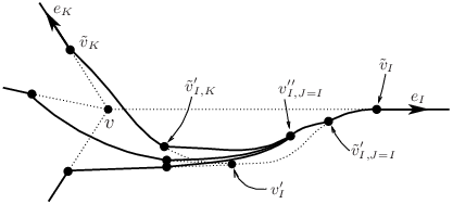
We imagine the deformed graph to be obtained by ‘pulling’ the original graph in the vicinity of the vertex $v$ “almost” along the direction of the edge $e_{I}$ . Thus new edges $\{\tilde{e}_{K}\}$ are obtained as the image of those parts of the old edges $\{{e}_{K}\}$ which are in the vicinity of the vertex $v$ . The new edges connect the displaced vertex to the old edges as follows (see Figure (1))

For $e_{I},$ we introduce a trivial vertex $\tilde{v}_{I}$ (on $e_{I}$ ), a coordinate distance $2\delta$ from $v,$ and adjoin the new $C^{k}$ -semianalytic edge $\tilde{e}_{I}$ which connects $\tilde{v}_{I}$ and $v_{I}^{\prime}.$ Since we want $\tilde{e}_{I}$ to “almost” overlap with (part of) the edge $e_{I}$ , we demand that the transition from $\tilde{e}_{I}$ to the original edge $e_{I}$ at $\tilde{v}_{I}$ be $C^{k}$ -violating in a strictly $C^{1}$ manner and that the tangent $\dot{\tilde{e}}{}_{I}^{a}$ at $v_{I}^{\prime}$ be proportional to $\dot{e}_{I}^{a}$ at $v$ (these vectors are comparable in the coordinate system $\{x\}$ ), i.e.:

\hat{\dot{\tilde{e}}}{}_{I}^{a}|_{v_{I}^{\prime}}=\hat{\dot{e}}{}_{I}^{a}|_{v}

(4.30)

We will refer to such vertices $\tilde{v}_{I}$ as $C^{1}$ -kink vertices or simply as $C^{1}$ -kinks.

Next, we introduce a coordinate ball $B_{\delta^{q}}(v)$ of radius $\delta^{q}$ about $v$ .

Note: We choose $q\geq 2,q<p$ . This choice is important for the technicalities of Appendix C.

For the remaining edges $e_{J\neq I},$ we introduce trivial vertices $\tilde{v}_{J}$ on all edges $e_{J}$ where they intersect $\partial B_{\delta^{q}}(v)$ ; that is, $\tilde{v}_{J}=e_{J}\cap\partial B_{\delta^{q}}(v).$ At $\tilde{v}_{J}$ introduce new $C^{k}$ -semianalytic edges $\tilde{e}_{J}$ which split off from each $e_{J}$ and head off to meet $v_{I}^{\prime}.$ These edges also ‘almost’ overlap (part of) the edge $e_{I}$ , reflecting our ‘singular pulling’ along of the vicinity of $v$ along the direction of the edge $e_{I}$ . As a result we require that the $C^{k}$ violation at $\tilde{v}_{J}$ be strictly $C^{0}$ . Such vertices $\tilde{v}_{J}$ will be referred to as $C^{0}$ -kink vertices or simply as $C^{0}$ -kinks.⁸⁸ 8 We note that the $C^{1}$ or $C^{0}$ nature of the kink is a diffeomorphism-invariant imprint of the graph deformation.

Since we imagine $\tilde{e}_{J}$ to be almost along $e_{I}$ , we require that the tangents of new edges $\tilde{e}_{J}$ at $v_{I}^{\prime}$ be ‘bunched’ around the direction $-\dot{\tilde{e}}_{I}$ at $v_{I}^{\prime}$ within a cone with apex angle of $O(\delta^{q-1})$ ( $q\geq 2$ ) with respect to $\{x\}$ ; i.e.

\hat{\dot{\tilde{e}}}^{a}_{J}|_{v_{I}^{\prime}}=-\hat{\dot{\tilde{e}}}^{a}_{I}|_{v_{I}^{\prime}}+O(\delta^{q-1}),

(4.31)

Refer to caption — Figure 1: A sample deformation produced by a single Hamiltonian constraint action at a non-degenerate vertex $v$ along the edge $e_{I}$ . The dashed edges emanating from the original vertex $v$ are now only charged in two of the three U(1) factors, but $v_{I}^{\prime}$ is expected to be, generically, non-degenerate. With respect to the coordinate system fixed at $v$ , $v_{I}^{\prime}$ is located a distance $\delta$ from $v$ along ${\dot{e}}_{I}$ and displaced off of $e_{I}$ a distance $O(\delta^{2})$ . $\tilde{e}_{I}$ and $e_{I}$ share a tangent at $\tilde{v}_{I}$ , but $\tilde{e}_{J}$ and $e_{J}$ do not share a tangent. All of the $\tilde{e}_{J\neq I}$ have tangents at $v_{I}^{\prime}$ which are ‘bunched’ and lie within a cone of apex angle $O(\delta^{q-1})$ .

Further, since we think of the deformation as some sort of ‘singular’ diffeomorphism, we require that some subset of diffeomorphism-invariant properties of the graph structure at $v$ be preserved by the new graph structure at the displaced vertex $v_{I}^{\prime}$ . In particular we require that if the set of edge tangents $\{\dot{e}_{K}^{a}\}$ at $v$ are such that no triple lie in a plane, the same should be true of the set $\{\dot{{\tilde{e}}}{}_{K}^{a}\}$ at $v_{I}^{\prime}$ . Vertices which such properties arise in the study of moduli in knot classes by Grot and Rovelli [15]. Grot and Rovelli call this property ‘non-degeneracy’. Accordingly we term such vertices as GR vertices. Thus, we require that the graph deformation preserve the GR nature of its vertices. Conversely, we also require that non-GR vertices do not acquire the GR property under graph deformation. We shall see that the GR property plays a key role in our analysis of diffeomorphism covariance [12].

Since we are thinking of the deformation as a (singular) diffeomorphism, we also require that no new non-trivial vertices are formed other than $v_{I}^{\prime}$ ; i.e., the new edges do not further intersect each other or the original graph. This may be explicitly achieved as follows.

Let the valence of $v$ be $M$ . Consider the $M$ new edges in some order $\tilde{e}_{I},\tilde{e}_{J_{1}},\tilde{e}_{J_{2}},..,\tilde{e}_{J_{M-1}},J_{k}\neq I$ . Let $\tilde{e}_{I}$ be a semianalytic curve which connects $\tilde{v}_{I}$ with $v_{I}^{\prime}$ in accordance with the requirements on its tangents at $\tilde{v}_{I}$ , $v_{I}^{\prime}$ . Let the coordinate plane (in the $\{x\}$ coordinates) which contains ${v_{I}^{\prime}}$ and which is normal to the direction $\hat{\dot{\tilde{e}}}_{I}^{a}|_{v_{I}^{\prime}}$ be $P$ . We require that the curve $\tilde{e}_{I}$ intersects $P$ only at $v_{I}^{\prime}$ so that $\tilde{e}_{I}$ is always “above” $P$ . As we show in Appendix C, for small enough $\delta$ we can always find such an (almost straight in $\{x\}$ ) curve. Let $\tilde{e}_{J_{1}}$ be a straight line in $\{x\}$ which connects $\tilde{v}_{J}$ with $v_{I}^{\prime}$ . If no unwanted intersections are produced, then we are done, and $\dot{\tilde{e}}_{J_{1}}$ at $v_{I}^{\prime}$ is approximately on the $O(\delta^{q-1})$ cone. If the so-constructed $\tilde{e}_{J_{1}}$ happens to produce an intersection at some (isolated because of the semianalyticity of the edges near $v$ , see Appendix C) point other than $\tilde{v}_{J_{1}}$ and $v_{I}^{\prime}$ , we can modify it with a bump function⁹⁹ 9 By this we mean that we can always apply, only to $\tilde{e}_{J_{1}}$ , a semi-analytic diffeomorphism which differs from the identity in a small enough compact set containing the intersection point so as to ‘lift’ $\tilde{e}_{J_{1}}$ away from the intersection point. Such a diffeomorphism can be generated by a vector field obtained by multiplying a semianalytic, appropriately transverse vector field with a semianalytic function of compact support. so that the intersection is avoided. It is always possible to tune the size of the bump so as to not produce any new unwanted intersection, nor destroy its tangent-near-on-cone property. We continue in this manner constructing each $\tilde{e}_{J_{K}}$ as a straight line, modifying this line with bumps where necessary. Since the ‘bumping’ is achieved via semianalytic diffeomorphisms, the new edges remain $C^{k}$ -semianalytic. It remains to show that the GR property (or lack thereof) of $v$ is preserved. First consider the case when $v$ is GR. Then if $v_{I}^{\prime}$ is GR we are done. If not, then as discussed further in Appendix C, we assume that the above prescription can be modified in a small vicinity of $v_{I}^{\prime}$ , without introducing any $C^{0}$ or $C^{1}$ kinks, in such a way as to render $v_{I}^{\prime}$ GR while still retaining the properties described by equations (4.29), (4.30), and (4.31). Indeed just such a prescription is constructed in detail in Reference [12] and we refer the interested reader to section 5.2 of that work. On the other hand, if $v$ is not GR, we show in Appendix C.3 that a minor modification of the prescription of the previous paragraph ensures that $v_{I}^{\prime}$ is also not GR.

Before we conclude this section, we note that the above prescriptions at triangulation fineness $\delta=\delta_{1}$ and at $\delta=\delta_{2}$ with $\delta_{2}<\delta_{1}$ are not necessarily related by a diffeomorphism. It turns out that for future considerations, such as the construction of the space of VSA states, as well as for our study of diffeomorphism covariance in [12], it is useful to construct prescriptions which are related by diffeomorphisms. In the appendix we show how this can be done in such a way that Equations (4.29), (4.30), and (4.31) continue to hold.

4.4.3 Charges

Since $\left[\cdots\right]_{\delta}^{I_{v},i}$ contains the difference between a deformed (and charge-flipped) charge network coordinate and its undeformed relative (but still with flipped charges), $\mathrm{e}^{\int\left[\cdots\right]_{\delta}^{I_{v},i}}$ contains the product of the deformed graph holonomy and the inverse of the undeformed relative, and so all edges of the graph holonomy $\mathrm{e}^{\int\left[\cdots\right]_{\delta}^{I_{v},i}}$ away from the deformation ‘erase’ each other. That is, the (colored) graph underlying $\mathrm{e}^{\int\left[\cdots\right]_{\delta}^{I_{v},i}}$ itself can be described simply by a gauge-invariant ‘pyramid skeleton’ consisting of the thin ‘star’ formed by $v$ and (for all original edges except the $I^{\text{th}}$ ) coordinate length $\delta^{q}$ edge segments from the original graph that connect $v$ and $\tilde{v}_{J}$ (for $e_{I},$ the contribution to the star has coordinate length $2\delta$ ). The charges on the star are minus the charge-flipped configuration charges; e.g., for the $i=1$ deformation, the star carries $\left(-q^{1},q^{3},-q^{2}\right)$ (with respect to an original coloring $\left(q^{1},q^{2},q^{3}\right)$ ) on each of its segments. The remaining edges (which meet $v^{\prime}$ ) carry the flipped charges $\left(q^{1},-q^{3},q^{2}\right).$ This pyramid charge network is multiplied by the original charge network $c(A)$ and, in our example of $i=1$ , the star part of the resulting state carries $\left(0,q^{2}+q^{3},q^{3}-q^{2}\right),$ which means that $v$ is now a zero-volume vertex (see Appendix A). A similar conspiration of the charges results for the other values of $i.$ Our $\hat{q}^{-1/3}$ will now annihilate this vertex (so the action of another Hamiltonian vanishes here).

We change notation slightly and drop from here on the prime on $\hat{C}^{\prime}$ . Equation (4.27) then reads

\hat{C}_{\delta}[N]c(A)=\frac{\hbar}{2\mathrm{i}}c(A)\sum_{v\in V(c)}\frac{3}{4\pi}N(x(v))\nu_{v}^{-2/3}\sum_{I_{v},i}q_{I_{v}}^{i}\frac{1}{\delta}\left(\exp\left({\textstyle\int}\left[\cdots\right]_{\delta}^{I_{v},i}\right)-1\right),

(4.32)

where we have made the regulating parameter $\delta$ explicit on the left hand side and dropped the $O(\delta)$ term. $\left[\cdots\right]_{\delta}^{I_{v},i}$ stands for the type of deformation described above (with charge flips). The charge configurations on the edges that meet at $v_{I}^{\prime}$ for the three quantum shifts $\vec{N}_{i}$ are

$\displaystyle\vec{N}_{1}$	$\displaystyle:\left(q^{1},-q^{3},q^{2}\right)$
$\displaystyle\vec{N}_{2}$	$\displaystyle:\left(q^{3},q^{2},-q^{1}\right)$	(4.33)
$\displaystyle\vec{N}_{3}$	$\displaystyle:\left(-q^{2},q^{1},q^{3}\right)$

We can write this compactly as

\left.{}^{(i)}\!q^{j}\right.=\delta^{ij}q^{j}-{\textstyle\sum\nolimits_{k}}\epsilon^{ijk}q^{k}

(4.34)

where $(i)$ specifies which shift $\vec{N}_{(i)}$ acted.

In the next section we evaluate the action of a second Hamiltonian constraint on the right hand side of Equation (4.32). In doing so it is of advantage to further improve our notation as follows. Denote the charge network corresponding to $\mathrm{e}^{\int_{\triangle_{\delta}(v)}\left[\cdots\right]_{\delta}^{I_{v},i}}c(A)$ by $c(i,v_{I_{v},\delta}^{\prime a}=\delta\hat{e}_{I_{v}}^{a}+\delta^{p}\hat{n}_{I_{v}}^{a})$ so that Equation (4.32) is written as:

\hat{C}_{\delta}[N]c(A)=\frac{\hbar}{2\mathrm{i}}\sum_{v\in V(c)}\frac{3}{4\pi}N(x(v))\nu_{v}^{-2/3}\sum_{I_{v},i}q_{I_{v}}^{i}\frac{1}{\delta}\left(c(i,v_{I_{v},\delta}^{\prime})-c\right)

(4.35)

The various quantifiers $\{I_{v},i,\delta\}$ in the argument of $c$ specify the particular edge $e_{I_{v}}$ emanating from $v$ along which the deformation (of magnitude $\sim\delta$ ) was performed, and the particular flipping of the charges via $i.$ Finally note that $\sum_{I_{v}}q_{I_{v}}^{i}=0$ by gauge invariance (all edges outgoing at $v$ ) so that:

\hat{C}_{\delta}[N]c(A)=\frac{\hbar}{2\mathrm{i}}\sum_{v\in V(c)}\frac{3}{4\pi}N(x(v))\nu_{v}^{-2/3}\sum_{I_{v},i}q_{I_{v}}^{i}\frac{1}{\delta}c(i,v_{I_{v},\delta}^{\prime})

(4.36)

4.5 Second Hamiltonian

We evaluate the action of a second regularized Hamiltonian constraint, smeared with a lapse $M$ on the right hand side of (4.36). Since we are interested in the continuum limit of (the action of VSA dual states on) the commutator, we drop those terms in $\hat{C}_{\delta^{\prime}}[M]\hat{C}_{\delta}[N]c(A)$ which vanish in the continuum limit upon the antisymmetrization of $N$ and $M$ and ‘contraction’ with a dual state. The dropped terms are those in which $\hat{C}_{\delta^{\prime}}[M]$ acts at vertices not moved by $\hat{C}_{\delta}[N]$ ; that is, the only contributions to the commutator will be from terms where $\hat{C}_{\delta^{\prime}}[M]$ acts at a vertex newly created by $\hat{C}_{\delta}[N]$ .¹⁰¹⁰ 10 The reader may easily verify this fact after the perusal of the next section.

Consider the term $\hat{C}_{\delta^{\prime}}[M]c(i,v_{I_{v},\delta}^{\prime})$ . Since $v$ now has vanishing inverse volume, the constraint acts at the displaced vertex $v_{I_{v},\delta}^{\prime}$ as well as on all other vertices of $c(i,v_{I_{v},\delta}^{\prime})$ which have non-vanishing inverse volume. But these other vertices are precisely the non-degenerate vertices of $c$ other than $v$ . As mentioned above, the contributions from these non-degenerate vertices vanish in the continuum limit evaluation of the commutator and so we do not display them here.

The deformations generated by the action of $\hat{C}_{\delta^{\prime}}[M]$ on $c(i,v_{I_{v},\delta}^{\prime})$ at the vertex $v_{I_{v},\delta}^{\prime}$ are defined in terms of the coordinate patch around $v_{I_{v},\delta}^{\prime}$ (see Section 4.4). We denote this coordinate system by $\{x^{\prime a^{\prime}}\}_{v_{I_{v},\delta}^{\prime}}$ or simply by $\{x^{\prime a^{\prime}}\}_{\delta}$ or just $\{x^{\prime}\}$ when the context is clear.

Note: In this work we require that in their region of joint validity $\{x_{\delta}^{{\prime}}\}$ and $\{x\}$ are related in a non-singular fashion as $\delta\rightarrow 0$ so that $\lim_{\delta\rightarrow 0}\{x^{\prime a^{\prime}}\}_{\delta}=:\{x^{\prime a^{\prime}}\}_{\delta=0}$ is a good coordinate system. Specifically, we require that the Jacobian matrix $J^{\mu}{}_{\nu^{\prime}}(x,x_{\delta}^{\prime}):=\partial x^{\mu}/\partial x_{\delta}^{\nu^{\prime}}$ is continuous in $\delta$ with non-vanishing and non-singular determinant.

It follows from the Note above that

\lim_{\delta\rightarrow 0}J^{\mu}{}_{\nu^{\prime}}(x,x_{\delta}^{\prime})=J^{\mu}{}_{\nu^{\prime}}(x,x_{\delta=0}^{\prime})

(4.37)

One possible way to construct such a set of coordinate patches is as follows: Since $\Sigma$ is compact, it can be covered by finitely-many coordinate charts. We pick one such set. Clearly (at least) one chart $\{x_{0}\}$ in this set covers a neighborhood of $v$ with ${\vec{x}}_{0}(v)$ being the coordinates of $v$ . Rigidly translate $\{x_{0}\}$ by ${\vec{x}}_{0}(v)$ to obtain obtain $\{x\}$ . For small enough $\delta$ , $\{x_{0}\}$ also covers small enough neighborhoods of the new vertices $v_{I_{v},\delta}^{\prime}$ with ${\vec{x}}_{0}(v_{I_{v},\delta}^{\prime})$ being the coordinates of $v_{I_{v},\delta}^{\prime}$ . Rigidly translate $\{x_{0}\}$ by ${\vec{x}}_{0}(v_{I_{v},\delta}^{\prime})$ to obtain $\{x^{\prime}\}_{\delta}$ . Clearly, this ensures that the Jacobian for the $\{x\}$ and $\{x^{\prime}\}_{\delta}$ charts is unity.¹¹¹¹ 11 This choice turns out to result in a conflict with diffeomorphism covariance; we shall comment on this in the concluding section and attempt to alleviate the problem in [12].

Recall that the edges $\{e_{J_{v}}\}$ at $v$ are deformed to the edges $\{{\tilde{e}}_{J_{v}}\}$ at $v_{I_{v},\delta}^{\prime}$ so that the valence of $v$ and $v_{I_{v},\delta}^{\prime}$ are equal and we may use the same index $J_{v}$ to enumerate the edges at $v$ and their counterparts at $v_{I_{v},\delta}^{\prime}$ . In what follows the primed index $a^{\prime}$ denotes components in the $\{x^{\prime}\}$ system and the primed ‘hat’ superscript, ^ˆ′, denotes unit norm as measured in the $\{x^{\prime}\}$ coordinate metric.

From Equation (4.8) the quantum shift eigenvalues at $v_{I_{v},\delta}^{\prime}$ are defined through:

\hat{M}_{i^{\prime}}^{a^{\prime}}(v_{I_{v},\delta}^{\prime})|c(i,v_{I_{v},\delta}^{\prime})\rangle=\sum_{J_{v}}\left.{}^{(i)}\!M_{i^{\prime}}^{a^{\prime}J_{v}}\right.(v_{I_{v},\delta}^{\prime})|c(i,v_{I_{v},\delta}^{\prime})\rangle,

(4.38)

and computed, via Equation (4.9) to be:

\left.{}^{(i)}\!M_{i^{\prime}}^{a^{\prime}J_{v}}\right.(v_{I_{v},\delta}^{\prime})=\frac{3}{4\pi}M(x_{\delta}^{\prime}(v_{I_{v},\delta}^{\prime}))\nu_{v_{I_{v},\delta}^{\prime}}^{-2/3}\left.{}^{(i)}\!q_{J_{v}}^{i^{\prime}}\right.\hat{\tilde{e}}^{\prime}{}_{J_{v}}^{a^{\prime}}

(4.39)

where $\hat{\tilde{e}}^{\prime}{}_{J_{v}}^{a^{\prime}}$ is the unit tangent to the edge ${\tilde{e}}_{J_{v}}$ at $v_{I_{v},\delta}^{\prime},$ and where we have used the fact that the inverse volume eigenvalue is independent of the charge flips inherent in the $i$ -dependence of $c(i,v_{I_{v},\delta}^{\prime})$ (see Appendix A). The term that survives the antisymmetrization and continuum limit is

\hat{C}_{\delta^{\prime}}[M]c(i,v_{I_{v},\delta}^{\prime})=\frac{\hbar}{2\mathrm{i}}\frac{3}{4\pi}M(x_{\delta}^{\prime}(v_{I_{v},\delta}^{\prime}))\nu_{v_{I_{v},\delta}^{\prime}}^{-2/3}\sum_{J_{v},i^{\prime}}\left.{}^{(i)}\!q_{J_{v}}^{i^{\prime}}\right.\frac{1}{\delta^{\prime}}(c(i,i^{\prime},v_{(I_{v},\delta),(J_{v},\delta^{\prime})}^{\prime\prime})-c(i,v_{I_{v},\delta}^{\prime}))

(4.40)

where the arguments of $c$ denote the deformation and charge flips determined by $\hat{C}_{\delta^{\prime}}[M].$ We detail their form below.

We distinguish two types of charge network that appear in the sum: $J_{v}=I_{v}$ and $J_{v}\neq I_{v}.$ Let $J_{v}=I_{v}$ (this situation is depicted in Figure (2)) and focus on the resulting charge network $c(i,i^{\prime},v_{(I_{v},\delta),I_{v},\delta^{\prime})}^{\prime\prime}).$ Following the prescription given above, $v_{I_{v},\delta}^{\prime}$ moves to (with respect to $\{x^{\prime}\}$ with origin at $v_{I_{v},\delta}^{\prime}$ )

v_{(I_{v},\delta),(I_{v},\delta^{\prime})}^{\prime\prime a^{\prime}}=\delta^{\prime}\hat{\tilde{e}}^{\prime}{}_{I_{v}}^{a^{\prime}}+\delta^{\prime p}\;\hat{n}_{I_{v}}^{\prime a^{\prime}}

(4.41)

for some ${\hat{n}}^{\prime}$ satisfying the conditions spelt out in Appendix C.

For $J_{v}\neq I_{v},$ $v_{I_{v},\delta}^{\prime}$ gets displaced along one of the ‘cone directions’ ${\hat{\tilde{e}}}{}_{J_{v}\neq I_{v}}^{\prime a^{\prime}}$ :

v_{(I_{v},\delta),(J_{v},\delta^{\prime})}^{\prime\prime a^{\prime}}=\delta^{\prime}{\hat{\tilde{e}}}{}_{J_{v}}^{\prime a^{\prime}}+\delta^{\prime p}{\;{\hat{n}}_{J_{v}}^{\prime a^{\prime}}}

(4.42)

The structure of the deformations are as described for the first action, but with $\delta$ replaced by $\delta^{\prime}.$ The particular charge configurations at $v^{\prime\prime}$ resulting from each possible sequence of charge flips is summarized in the following table:

	$i=1$	$i=2$	$i=3$
$i^{\prime}=1$	$\left(q^{1},-q^{2},-q^{3}\right)$	$\left(q^{3},q^{1},q^{2}\right)$	$\left(-q^{2},-q^{3},q^{1}\right)$
$i^{\prime}=2$	$\left(q^{2},-q^{3},-q^{1}\right)$	$\left(-q^{1},q^{2},-q^{3}\right)$	$\left(q^{3},q^{1},q^{2}\right)$
$i^{\prime}=3$	$\left(q^{3},q^{1},q^{2}\right)$	$\left(-q^{2},q^{3},-q^{1}\right)$	$\left(-q^{1},-q^{2},q^{3}\right)$

(4.43)

Thus

		$\displaystyle\hat{C}_{\delta^{\prime}}[M]\hat{C}_{\delta}[N]c$
		$\displaystyle=\frac{\hbar}{2\mathrm{i}}\sum_{v\in V(c)}\frac{3}{4\pi}N(x(v))\nu_{v}^{-2/3}\sum_{I_{v},i}q_{I_{v}}^{i}\frac{1}{\delta}\hat{C}_{\delta^{\prime}}[M]c(i,v_{I_{v},\delta}^{\prime})$
		$\displaystyle=\left(\frac{\hbar}{2\mathrm{i}}\frac{3}{4\pi}\right)^{2}\sum_{v\in V(c)}\frac{1}{\delta\delta^{\prime}}N(x(v))\nu_{v}^{-2/3}\sum_{I_{v}}\nu_{v_{I_{v}}^{\prime}}^{-2/3}\sum_{i}q_{I_{v}}^{i}$		(4.44)
		$\displaystyle\qquad\qquad\times\sum_{J_{v},i^{\prime}}\left(\delta^{ii^{\prime}}q_{J_{v}}^{i^{\prime}}-{\textstyle\sum\nolimits_{j}}\epsilon^{ii^{\prime}j}q_{J_{v}}^{j}\right)M(x_{\delta}^{\prime}(v_{I_{v},\delta}^{\prime}))c(i,i^{\prime},v_{(I_{v},\delta),(J_{v},\delta^{\prime})}^{\prime\prime}).$

Above, we have used gauge invariance to set $\sum_{J_{v}}\left.{}^{(i)}\!q_{J_{v}}^{i^{\prime}}\right.=0$ . We have also set $\nu_{v_{I_{v},\delta}^{\prime}}^{-2/3}\equiv\nu_{v_{I_{v}}^{\prime}}^{-2/3}$ ; this follows from the diffeomorphism invariance of the inverse metric eigenvalue (see Appendix A) together with the fact that the deformations at different values of $\delta$ are related by diffeomorphisms (see Appendix C.4).

4.6 Continuum Limit

In this section we evaluate the continuum limit of the commutator between a pair of finite triangulation Hamiltonian constraints under certain assumptions with regard to the properties of the VSA states. In Section 6 we shall construct a large class of VSA states which satisfy these assumptions. As mentioned in Section 3.1, the VSA states are weighted sums over certain bra states. As we shall see in Section 6, the weights are obtained by the evaluation of a smooth complex-valued function $f$ on the non-degenerate ¹²¹² 12 We assume that the deformed vertices created by the Hamiltonian constraint are nondegenerate (i.e. have non- vanishing inverse volume) in the deformed chargenet if their undeformed counterparts are nondegenerate in the undeformed chargenet. While we expect this to be generically true, it is possible that this assumption is violated. However, the assumption is made only for pedagogy. As the interested reader may verify (after a perusal of section 6), it suffices to replace this non- degeneracy property by the property that the vertex is GR, has valence greater than 3 and that there exists no $i$ such that the $i^{\rm th}$ charge vanishes on all edges emanating from it. vertices of the bra it multiplies. More precisely, all bras in the sum have the same number $n$ of non-degenerate vertices and the evaluation of $f:\Sigma^{n}\rightarrow\mathbf{\mathbb{C}}$ on the $n$ points corresponding to the $n$ non-degenerate vertices of the bra, provides the weight of that bra in the sum:

(\Psi_{B_{\mathrm{VSA}}}^{f}|~:=\sum_{\bar{c}\in B_{\mathrm{VSA}}}\kappa_{\bar{c}}f(V(\bar{c}))\langle\bar{c}|

(4.45)

For simplicity we restrict attention to those ${\bar{c}}$ such that there is no symmetry of ${\bar{c}}$ which interchanges its nondegenerate vertices. We will sometimes write $\Psi(c):=(\Psi|c\rangle.$ In (4.45), $\Psi_{B_{\mathrm{VSA}}}^{f}$ is a VSA state, $B_{\mathrm{VSA}}$ is the set of bras being summed over, $V(\bar{c})$ denotes the set of non-degenerate vertices of ${\bar{c},}$ and we have introduced the ${\bar{c}}$ -dependent real number $\kappa_{\bar{c}}$ into the expression. To avoid notational clutter we have suppressed the $\kappa_{\bar{c}}$ dependence in $(\Psi_{B_{\mathrm{VSA}}}^{f}|$ . The continuum limit of the commutator is

\lim_{\delta\rightarrow 0}\lim_{\delta^{\prime}\rightarrow 0}\Psi^{f}_{B_{\mathrm{VSA}}}(({\hat{C}}_{\delta^{\prime}}[M]{\hat{C}}_{\delta}[N]-{\hat{C}}_{\delta^{\prime}}[N]{\hat{C}}_{\delta}[M])c).

(4.46)

Using Equation (4.40), we first evaluate $\lim_{\delta^{\prime}\rightarrow 0}\Psi^{f}_{B_{\mathrm{VSA}}}({\hat{C}}_{\delta^{\prime}}[M]c(i,v_{I_{v},\delta}^{\prime}))$ . We have that

\Psi_{B_{\mathrm{VSA}}}(\hat{C}_{\delta^{\prime}}[M]c(i,v_{I_{v},\delta}^{\prime}))=\frac{\hbar}{2\mathrm{i}}\frac{3}{4\pi}M(x_{\delta}^{\prime}(v_{I_{v},\delta}^{\prime}))\nu_{v_{I_{v}}}^{-2/3}\sum_{J_{v},i^{\prime}}\left.{}^{(i)}\!q_{J_{v}}^{i^{\prime}}\right.\frac{1}{\delta^{\prime}}(\Psi_{B_{\mathrm{VSA}}}(c(i,i^{\prime},v_{(I_{v},\delta),(J_{v},\delta^{\prime})}^{\prime\prime}))

(4.47)

where we have set $\nu_{v_{I_{v},\delta}^{\prime}}=\nu_{v_{I_{v}}}$ and used gauge invariance to drop the last term:

\sum_{J_{v}}q_{I_{v}}^{i}=0=\sum_{J_{v}}\left.{}^{(i)}\!q_{J_{v}}^{i^{\prime}}\right.

(4.48)

Next, we make the following assumptions which will be shown to hold in Section 6:

(1)

For a point $v\in\Sigma$ and a charge network $c$ , either there exists $\delta_{0}(c)\equiv\delta_{0}$ such that $\forall\delta<\delta_{0}$ there exists $\delta_{0}^{\prime}(\delta)$ such that $\forall\delta^{\prime}<\delta_{0}^{\prime}(\delta)$ we have that

\{\langle c(i,i^{\prime},v_{(I_{v},\delta),(J_{v},\delta^{\prime})}^{\prime\prime})~|~\forall~i,i^{\prime},I_{v},J_{v}\}\subset B_{\mathrm{VSA}},

(4.49)

or $\forall\delta,\delta^{\prime}$ for which $c(i,i^{\prime},v_{(I_{v},\delta),(J_{v},\delta^{\prime})}^{\prime\prime})$ is defined we have that:

\{\langle c(i,i^{\prime},v_{(I_{v},\delta),(J_{v},\delta^{\prime})}^{\prime\prime})~|~\forall~i,i^{\prime},I_{v},J_{v}\}\cap B_{\mathrm{VSA}}=\emptyset.

(4.50)

(2)

If Equation (4.49) holds, then

$\kappa_{c(i,i^{\prime},v_{(I_{v},\delta),(J_{v},\delta^{\prime})}^{\prime\prime})}=1\qquad\forall~i,i^{\prime},I_{v},J_{v}$ (4.51)

If (4.50) holds, the right hand side of (4.47) vanishes. We shall see in Section 6 that in this case, the corresponding ‘matrix element’ for the RHS also vanishes. We continue the calculation in the case that (4.49) holds. We have that:

\Psi_{B_{\mathrm{VSA}}}(\hat{C}_{\delta^{\prime}}[M]c(i,v_{I_{v},\delta}^{\prime}))=\frac{\hbar}{2\mathrm{i}}\frac{3}{4\pi}M(x_{\delta}^{\prime}(v_{I_{v},\delta}^{\prime}))\nu_{v_{I_{v}}}^{-2/3}\sum_{J_{v},i^{\prime}}\left.{}^{(i)}\!q_{J_{v}}^{i^{\prime}}\right.\frac{1}{\delta^{\prime}}(f(v_{(I_{v},\delta),(J_{v},\delta^{\prime})}^{\prime\prime})-f(v_{I_{v},\delta}^{\prime}))

(4.52)

where, once again we have used gauge invariance to append the term $f(v_{I_{v},\delta}^{\prime})$ . In addition for notational convenience only displayed the dependence of $f$ on the (doubly and singly) deformed images of $v$ and suppressed its dependence on the undeformed vertices. Using (4.41), (4.42) and the smoothness of $f$ , we obtain

\lim_{\delta^{\prime}\rightarrow 0}\Psi_{B_{\mathrm{VSA}}}(\hat{C}_{\delta^{\prime}}[M]c(i,v_{I_{v},\delta}^{\prime}))=\frac{\hbar}{2\mathrm{i}}\frac{3}{4\pi}M(x_{\delta}^{\prime}(v_{I_{v},\delta}^{\prime}))\nu_{v_{I_{v}}}^{-2/3}\sum_{J_{v},i^{\prime}}\left.{}^{(i)}\!q_{J_{v}}^{i^{\prime}}\right.({\hat{\tilde{e}}}{}_{J_{v}}^{\prime})^{a}\partial_{a}f(v_{I_{v},\delta}^{\prime})

(4.53)

where $({\hat{\tilde{e}}}{}_{J_{v}}^{\prime})^{a}$ is the component of the unit vector $\vec{{\hat{\tilde{e}}}}{}_{J_{v}}^{\prime}$ in the $\{x\}$ coordinate system. Here the vector $\vec{{\hat{\tilde{e}}}}{}_{J_{v}}^{\prime}$ is obtained by normalizing the tangent vector to the edge ${\tilde{e}}_{J_{v}}$ at $v_{I_{v},\delta}^{\prime}$ in the $\{x^{\prime}\}$ system (recall, from (4.41), (4.42) that the components of this vector in the $\{x^{\prime}\}$ system are given by $({\hat{\tilde{e}}}{}_{J_{v}}^{\prime})^{a^{\prime}}$ ).

It follows from the above equation in conjunction with (4.44) that

	$\displaystyle\lim_{\delta^{\prime}\rightarrow 0}\Psi_{B_{\mathrm{VSA}}}(\hat{C}_{\delta^{\prime}}[M]\hat{C}_{\delta}[N]c)$	$\displaystyle=\left(\frac{\hbar}{2\mathrm{i}}\frac{3}{4\pi}\right)^{2}\frac{1}{\delta}\sum_{v}\nu_{v}^{-2/3}N(x(v))\sum_{I_{v}}M(x_{\delta}^{\prime}(v_{I_{v},\delta}^{\prime}))$
		$\displaystyle\qquad\times\sum_{i}q_{I_{v}}^{i}\nu_{v_{I_{v}}}^{-2/3}\sum_{J_{v},i^{\prime}}\left.{}^{(i)}\!q_{J_{v}}^{i^{\prime}}\right.({\hat{\tilde{e}}}{}_{J_{v}}^{\prime})^{a}\partial_{a}f(v_{I_{v},\delta}^{\prime}).$		(4.54)

Since $M$ is of density weight $-1/3$ we have:

M(x_{\delta}^{\prime}(v_{I_{v},\delta}^{\prime}))=M(x(v_{I_{v},\delta}^{\prime}))\left[\det\left(\frac{\partial x}{\partial x^{\prime}}\right)_{v_{I_{v},\delta}^{\prime}}\right]^{-1/3}.

(4.55)

Using this, we obtain

	$\displaystyle\lim_{\delta^{\prime}\rightarrow 0}\Psi_{B_{\mathrm{VSA}}}(\hat{C}_{\delta^{\prime}}[M]\hat{C}_{\delta}[N]c)$	$\displaystyle=\left(\frac{\hbar}{2\mathrm{i}}\frac{3}{4\pi}\right)^{2}\frac{1}{\delta}\sum_{v}\nu_{v}^{-2/3}N(x(v))$		(4.56)
		$\displaystyle\qquad\times\sum_{I_{v}}M(x(v_{I_{v},\delta}^{\prime}))\left[\det\left(\frac{\partial x}{\partial x^{\prime}}\right)_{v_{I_{v},\delta}^{\prime}}\right]^{-1/3}\{\cdots\}_{I_{v},\delta}$

where

\{\cdots\}_{I_{v},\delta}:=\sum_{i}q_{I_{v}}^{i}\nu_{v_{I_{v}}}^{-2/3}\sum_{J_{v},i^{\prime}}\left.{}^{(i)}\!q_{J_{v}}^{i^{\prime}}\right.({\hat{\tilde{e}}}{}_{J_{v}}^{\prime})^{a}\partial_{a}f(v_{I_{v},\delta}^{\prime})

(4.57)

Next, we use (4.29) to Taylor expand $M$ as:

M(x(v_{I,\delta}^{\prime}))=M(x(v))+(\delta\hat{e}_{I_{v}}^{a})\partial_{a}M(x(v))+O(\delta^{2}).

(4.58)

Using the above Equation in (4.56) to evaluate the commutator, we obtain in ‘bra-ket’ notation:

		$\displaystyle\lim_{\delta^{\prime}\rightarrow 0}(\Psi_{B_{\mathrm{VSA}}}\|(\hat{C}_{\delta^{\prime}}[M]\hat{C}_{\delta}[N]-\left(N\leftrightarrow M\right))\|c\rangle$
		$\displaystyle=\left(\frac{\hbar}{2\mathrm{i}}\frac{3}{4\pi}\right)^{2}\sum_{v}\nu_{v}^{-2/3}$
		$\displaystyle\qquad\times\sum_{I_{v}}\{N(x(v))\hat{e}_{I_{v}}^{a}\partial_{a}M(x(v))-\left(N\leftrightarrow M\right)+O(\delta)\}\left[\det\left(\frac{\partial x}{\partial x^{\prime}}\right)_{v_{I_{v},\delta}^{\prime}}\right]^{-1/3}\{\cdots\}_{I_{v},\delta}$		(4.59)

We now compute the $\delta\rightarrow 0$ limit of the above equation so as to obtain the continuum limit of the commutator. By virtue of the smooth dependence of $x$ on $x_{\delta}^{\prime}$ (see the note in Section 4.5) the determinant is a continuous function of $\delta$ . It remains to compute the $\delta\rightarrow 0$ limit of $\{\cdots\}_{I_{v},\delta}$ .

Since the $\{x\}$ and $\{x^{\prime}\}\equiv\{x^{\prime}\}_{\delta}$ systems are not necessarily the same, we have that $({\hat{\tilde{e}}}{}_{J_{v}}^{\prime})^{a}$ is proportional to $({\hat{\tilde{e}}}_{J_{v}})^{a}|_{v_{I_{v},\delta}^{\prime}}$ where now the same tangent vector has been normalized in the $\{x\}$ system. From the Note and equation (4.37) in Section 4.5, in conjunction with Equations (4.31) in Section 4.4.2, we have that that at $v_{I_{v},\delta}^{\prime}$ , for $J_{v}\neq I_{v}$

{\hat{\tilde{e}}}{}_{J_{v}}^{\prime a}=-{\hat{\tilde{e}}}{}_{I_{v}}^{\prime a}+O(\delta^{q-1}),\qquad q\geq 2.

(4.60)

Using this in (4.57) together with the smoothness of $\partial_{a}f$ , we obtain

\{\cdots\}_{I_{v},\delta}=\nu_{v_{I_{v}}}^{-2/3}\sum_{i}q_{I_{v}}^{i}\sum_{i^{\prime}}\left(\left.{}^{(i)}\!q_{I_{v}}^{i^{\prime}}\right.-\sum_{J_{v}\neq I_{v}}\left.{}^{(i)}\!q_{J_{v}}^{i^{\prime}}\right.\right)({\hat{\tilde{e}}}{}_{I_{v}}^{\prime})^{a}\partial_{a}f(v_{I_{v},\delta}^{\prime})+O(\delta)

(4.61)

Gauge invariance (4.48) then implies that:

\{\cdots\}_{I_{v},\delta}:=2\nu_{v_{I_{v}}}^{-2/3}\sum_{i}q_{I_{v}}^{i}\sum_{i^{\prime}}\left.{}^{(i)}\!q_{I_{v}}^{i^{\prime}}\right.({\hat{\tilde{e}}}{}_{I_{v}}^{\prime})^{a}\partial_{a}f(v_{I_{v},\delta}^{\prime})+O(\delta)

(4.62)

Finally, from (4.34) it follows that

\lim_{\delta\rightarrow 0}\{\cdots\}_{I_{v},\delta}:=2\nu_{v_{I_{v}}}^{-2/3}\sum_{i}(q_{I_{v}}^{i})^{2}({\hat{\tilde{e}}}{}_{I_{v}}^{\prime})^{a}\partial_{a}f(v)

(4.63)

Up to this point we have refrained from assuming any particular relation between $\{x_{\delta=0}^{\prime}\}$ and $\{x\}$ in order to exhibit the structure of the calculation as $\delta\rightarrow 0$ . Section 4.1 together with equation (4.37) implies that the Jacobian between the two coordinate systems is the identity:

\frac{\partial x_{\delta=0}^{\prime\mu}}{\partial x^{\nu}}=\delta_{\nu}^{\mu}.

(4.64)

Using this together with (4.63) and (4.59) we obtain the continuum limit of the commutator under the assumption (4.49) to be:

		$\displaystyle(\Psi_{B_{\mathrm{VSA}}}^{f}\|[\hat{C}[M],\hat{C}[N]]\|c\rangle$
		$\displaystyle=\lim_{\delta\rightarrow 0}\lim_{\delta^{\prime}\rightarrow 0}(\Psi_{B_{\mathrm{VSA}}}^{f}\|(\hat{C}_{\delta^{\prime}}[M]\hat{C}_{\delta}[N]-\left(N\leftrightarrow M\right))\|c\rangle$
		$\displaystyle=2\left(\frac{\hbar}{2\mathrm{i}}\frac{3}{4\pi}\right)^{2}\sum_{v\in V(c)}\sum_{I_{v},i}(q_{I_{v}}^{i})^{2}\nu_{v}^{-2/3}\nu_{v_{I_{v}}}^{-2/3}\hat{e}_{I_{v}}^{a}\hat{e}_{I_{v}}^{b}\left(N\partial_{a}M-M\partial_{a}N\right)(x(v))\partial_{b}f(v)$		(4.65)

5 RHS

In Section 5.1 we display a remarkable classical identity which expresses the RHS as the Poisson bracket between a pair of diffeomorphism constraints, each smeared with an electric shift. This implies, that in the quantum theory, we may identify the RHS with commutator between two such constraints. Accordingly, in Section 5.2 we construct the finite triangulation operator corresponding to single diffeomorphism constraint smeared with an electric shift using arguments which parallel those of Section 4. We compute the finite-triangulation commutator between two such operators in Section 5.3. We compute the continuum limit of this commutator in Section 5.4 under certain assumptions (whose validity is demonstrated in Section 6) on the VSA states.

5.1 A Remarkable Identity

It is straightforward to check that for

H[N]=\tfrac{1}{2}\int\mathrm{d}^{3}x~\frac{N}{q^{\alpha}}\epsilon^{ijk}E_{i}^{a}E_{j}^{b}F_{ab}^{k},

(5.1)

we have

\{H[M],H[N]\}=\int\mathrm{d}^{3}x~\left(N\partial_{c}M-M\partial_{c}N\right)\frac{E_{i}^{c}E_{i}^{b}}{q^{2\alpha}}F_{ba}^{j}E_{j}^{a}=:D[\vec{\omega}],

(5.2)

where

\omega^{a}:=\left(N\partial_{b}M-M\partial_{b}N\right)q^{-2\alpha}E_{i}^{b}E_{i}^{a}.

Let the diffeomorphism generator smeared with the “electric shift” (see Section 4.3), $N_{i}^{a}:=q^{-\alpha}NE_{i}^{a}$ , be denoted $D[\vec{N}_{i}]$ :

D[\vec{N}_{i}]=\int\mathrm{d}^{3}x~q^{-\alpha}NE_{i}^{a}F_{ab}^{j}E_{j}^{b},

(5.3)

We shall refer to $D[\vec{N}_{i}]$ as an electric diffeomorphism constraint. The Poisson bracket between a pair of electric diffeomorphism constraints is (summing over the internal index $i$ ):

		$\displaystyle\{D[\vec{M}_{i}],D[\vec{N}_{i}]\}$
		$\displaystyle=\int\mathrm{d}^{3}x~\left(\frac{\delta D[\vec{M}_{i}]}{\delta A_{a}^{j}(x)}\frac{\delta D[\vec{N}_{i}]}{\delta E_{j}^{a}(x)}-\left(N\leftrightarrow M\right)\right)$
		$\displaystyle=-\int\mathrm{d}^{3}x~2\delta_{[c}^{a}\partial_{b]}\left(\frac{ME_{i}^{b}}{q^{\alpha}}E_{j}^{c}\right)\left(\frac{NE_{k}^{b^{\prime}}}{q^{\alpha}}\delta_{i}^{j}F_{ab^{\prime}}^{k}-\frac{NE_{i}^{b^{\prime}}}{q^{\alpha}}F_{ab^{\prime}}^{j}+\int\mathrm{d}^{3}y~NE_{i}^{b^{\prime}}F_{b^{\prime}c^{\prime}}^{k}E_{k}^{c^{\prime}}\frac{\delta q^{-\alpha}(y)}{\delta E_{j}^{a}(x)}\right)$
		$\displaystyle\qquad\qquad\qquad\qquad-\left(N\leftrightarrow M\right)$
		$\displaystyle=\int\mathrm{d}^{3}x~\left(\frac{E_{j}^{a}E_{i}^{b}}{q^{\alpha}}\frac{E_{i}^{c}}{q^{\alpha}}F_{ac}^{j}N\partial_{b}M+\frac{2E_{[i}^{a}E_{j]}^{b}}{q^{\alpha}}\partial_{b}M\int\mathrm{d}^{3}y~NE_{i}^{b^{\prime}}F_{b^{\prime}c^{\prime}}^{k}E_{k}^{c^{\prime}}\frac{\delta q^{-\alpha}(y)}{\delta E_{j}^{a}(x)}-\left(N\leftrightarrow M\right)\right)$		(5.4)
		$\displaystyle=\int\mathrm{d}^{3}x~\left(\frac{E_{i}^{b}E_{i}^{c}}{q^{2\alpha}}F_{ca}^{j}E_{j}^{a}-2\alpha\frac{E_{i}^{b}E_{i}^{b^{\prime}}}{q^{2\alpha}}F_{b^{\prime}c^{\prime}}^{k}E_{k}^{c^{\prime}}\right)\left(M\partial_{b}N-N\partial_{b}M\right)$
		$\displaystyle=\left(1-2\alpha\right)\int\mathrm{d}^{3}x~\left(M\partial_{b}N-N\partial_{b}M\right)\frac{E_{i}^{b}E_{i}^{c}}{q^{2\alpha}}F_{ca}^{j}E_{j}^{a}$
		$\displaystyle=\left(2\alpha-1\right)D[\vec{\omega}],$

in which we have used

\frac{\delta q^{\alpha}(y)}{\delta E_{i}^{a}(x)}=\alpha q^{\alpha}(E^{-1})_{a}^{i}(y)\delta^{(3)}(x,y),

(5.5)

where $(E^{-1})_{a}^{i}$ is the ‘inverse’ of $E_{j}^{b}$ so that $E_{a}^{i}E_{i}^{b}=\delta_{a}^{b},E_{a}^{i}E_{j}^{a}=\delta_{j}^{i}$ . Thus we may write the RHS as

\{H[M],H[N]\}=\frac{1}{2\alpha-1}\sum_{i=1}^{3}\{D[\vec{M}_{i}],D[\vec{N}_{i}]\}.

(5.6)

In this work we are interested in $\alpha=\frac{1}{3}$ (see Equation (4.1)). In Section 5.4 we use this identity to express the RHS operator as the commutator between two finite diffeomorphism operators. As mentioned in Section 3.1 (see Step 3 of that section), this facilitates the comparison of the LHS and RHS operators.

Note that this identity trivializes precisely for the case $\alpha=\frac{1}{2}$ ; this is the case of Hamiltonian constraints of density weight one considered hitherto in the literature. We take this trivialization as further support for the move away from the density one case. We also note that, as shown in Appendix B, this identity holds for the SU $(2)$ case in $2+1$ and $3+1$ dimensions and in all cases trivializes for the density weight one choice.

5.2 The Electric Diffeomorphism Constraint Operator at Finite Triangulation

We set $\alpha=\frac{1}{3}$ in (5.3). Modulo Gauss law terms we have that:

D[{\vec{N}}_{i}]=\int_{\Sigma}\mathrm{d}^{3}x(\pounds_{\vec{N}_{i}}A_{b}^{j})E_{j}^{b}

(5.7)

where ${\vec{N}}_{i}$ is the electric shift of Section 4. This motivates, analogous to (4.14), the following heuristic operator action

{\hat{D}}[{\vec{N}}_{i}]c(A)=-\frac{\hbar}{\mathrm{i}}c(A)\int_{\Sigma}\mathrm{d}^{3}x(\pounds_{\vec{N}_{i}}c_{i}^{a})A_{a}^{i}

(5.8)

Following an argumentation similar to that between Equations (4.14)-(4.24) leads us to the finite-triangulation electric diffeomorphism constraint operator action:

	$\displaystyle\hat{D}_{\delta}[\vec{N}_{i}]c$	$\displaystyle=\frac{\hbar}{\mathrm{i}}\frac{3}{4\pi}\sum_{v}N(x(v))\nu_{v}^{-2/3}\sum_{I_{v}}q_{I_{v}}^{i}\frac{1}{\delta}(c(v_{I_{v},\delta}^{\prime})-c)$
		$\displaystyle=\frac{\hbar}{\mathrm{i}}\frac{3}{4\pi}\sum_{v}N(x(v))\nu_{v}^{-2/3}\sum_{I_{v}}q_{I_{v}}^{i}\frac{1}{\delta}c(v_{I_{v},\delta}^{\prime})$		(5.9)

where we have used gauge invariance to drop the “ $-c$ ” term in the second line and where the charge network coordinate underlying the state $c(v_{I_{v},\delta}^{\prime})$ is given by

(c_{v_{I_{v},\delta}^{\prime}})_{i}^{a}(x):=\varphi(\vec{{\hat{e}}}_{I},\delta)^{\ast}c_{i}^{a}(x)

(5.10)

where $\varphi(\vec{{\hat{e}}}_{I},\delta)$ deforms the graph underlying $c$ in the manner discussed in Section 4.4. More in detail, the graph underlying $c(v_{I_{v},\delta}^{\prime})$ is obtained by removing the segments of the graph underlying $c$ which connect $v$ to the points ${\tilde{v}}_{J}$ and adjoining new edges, ${\tilde{e}}_{J}$ which connect ${\tilde{v}}_{J}$ to the displaced vertex $v_{I_{v},\delta}^{\prime}$ as explained in Section 4.4. The deformed graph is identical to the one shown in Figure (1), but with the dashed edges removed. Also note that since $D[{\vec{N}}_{i}]$ is constructed by smearing the diffeomorphism constraint with an electric shift, the edges ${\tilde{e}}_{J}$ carry the same charges as $e_{J}$ i.e. there are no “charge flips”.

5.3 Second Electric Diffeomorphism

We evaluate the action of a second electric diffeomorphism constraint, smeared with the electric shift ${\vec{M}}_{i}$ on the right hand side of (5.9). Since we are interested in the continuum limit of (the action of VSA dual states on) the commutator between two electric diffeomorphism constraints, we drop those terms in $\hat{D}_{\delta^{\prime}}[{\vec{M}}_{i}]\hat{D}_{\delta}[{\vec{N}}_{i}]c(A)$ which vanish in the continuum limit upon the antisymmetrization of $N$ and $M$ . The dropped terms are those in which $\hat{D}_{\delta^{\prime}}[{\vec{M}}_{i}]$ acts at vertices not moved by $\hat{D}_{\delta}[{\vec{N}}_{i}]$ ; that is, the only contributions to the commutator will be from terms where $\hat{D}_{\delta^{\prime}}[{\vec{M}}_{i}]$ acts at a vertex which has been moved by $\hat{D}_{\delta}[{\vec{N}}_{i}]$ . Consider the term $\hat{D}_{\delta^{\prime}}[{\vec{M}}_{i}]c(v_{I_{v},\delta}^{\prime})$ . The constraint acts at the displaced vertex $v_{I_{v},\delta}^{\prime}$ as well as on all other vertices of $c(v_{I_{v},\delta}^{\prime})$ which have non-vanishing inverse volume. But these other vertices are precisely the non-degenerate vertices of $c$ other than $v$ . As mentioned above, the contributions from these non-degenerate vertices vanish in the continuum limit evaluation of the commutator and so we do not display them here.

The deformations generated by the action of $\hat{D}_{\delta^{\prime}}[{\vec{M}}_{i}]$ on $c(v_{I_{v},\delta}^{\prime})$ at the vertex $v_{I_{v},\delta}^{\prime}$ are, as in the case of Hamiltonian constraint of Section 4.4, defined in terms of the coordinate patch $\{x^{\prime}\}$ around $v_{I_{v},\delta}^{\prime}$ . From Equation (4.8), we have that

{\hat{M}}_{i}^{a^{\prime}}(v_{I_{v},\delta}^{\prime})|c(v_{I_{v},\delta}^{\prime})\rangle=\sum_{J_{v}}M_{i}^{a^{\prime}J_{v}}(v_{I_{v},\delta}^{\prime})|c(v_{I_{v},\delta}^{\prime})\rangle,

(5.11)

with $M_{i}^{a^{\prime}J_{v}}(v_{I_{v},\delta}^{\prime})$ given by

M_{i}^{a^{\prime}J_{v}}(v_{I_{v},\delta}^{\prime})=\frac{3}{4\pi}M(x_{\delta}^{\prime}(v_{I_{v},\delta}^{\prime}))\nu_{v_{I_{v},\delta}^{\prime}}^{-2/3}q_{J_{v}}^{i}{{\hat{\tilde{e}}}}{}^{\prime}{{}_{J_{v}}^{a^{\prime}}}

(5.12)

The term that survives the antisymmetrization and continuum limit is

	$\displaystyle\hat{D}_{\delta^{\prime}}[{\vec{M}}_{i}]c(v_{I_{v},\delta}^{\prime})$	$\displaystyle=\frac{\hbar}{\mathrm{i}}\frac{3}{4\pi}M(x_{\delta}^{\prime}(v_{I_{v},\delta}^{\prime}))\nu_{v_{I_{v},\delta}^{\prime}}^{-2/3}\sum_{J_{v}}q_{J_{v}}^{i}\frac{1}{\delta^{\prime}}(c(v_{(I_{v},\delta),(J_{v},\delta^{\prime})}^{\prime\prime})-c(v_{I_{v},\delta}^{\prime}))$
		$\displaystyle=\frac{\hbar}{\mathrm{i}}\frac{3}{4\pi}M(x_{\delta}^{\prime}(v_{I_{v},\delta}^{\prime}))\nu_{v_{I_{v},\delta}^{\prime}}^{-2/3}\sum_{J_{v}}q_{J_{v}}^{i}\frac{1}{\delta^{\prime}}c(v_{(I_{v},\delta),(J_{v},\delta^{\prime})}^{\prime\prime})$		(5.13)

where we have used gauge invariance to drop the last term in the second line. Here $c(v_{(I_{v},\delta),(J_{v},\delta^{\prime})}^{\prime\prime})$ denotes the charge network state obtained by deforming the state $c(v_{I_{v},\delta}^{\prime})$ by the ‘singular’ diffeomorphism generated by $\hat{D}_{\delta^{\prime}}[{\vec{M}}_{i}]$ . The deformation moves the vertex $v_{I_{v},\delta}^{\prime}$ of $c(v_{I_{v},\delta}^{\prime})$ to its new position, $v_{(I_{v},\delta),(J_{v},\delta^{\prime})}^{\prime\prime}$ given by Equation (4.41) when $J_{v}=I_{v}$ and by Equation (4.42) when $J_{v}\neq I_{v}$ . The structure of the deformations are as described for the first action in Section 5.2, but with $\delta\rightarrow\delta^{\prime}$ (see Figure (3)).

Restoring the sum over vertices we have, modulo terms which vanish upon antisymmetrization in the lapses and the taking of the continuum limit:

	$\displaystyle\hat{D}_{\delta^{\prime}}[\vec{M}_{i}]\hat{D}_{\delta}[\vec{N}_{i}]c$	$\displaystyle=\left(\frac{\hbar}{\mathrm{i}}\frac{3}{4\pi}\right)\sum_{v}\frac{1}{\delta}N(x(v))\nu_{v}^{-2/3}\sum_{I_{v}}q_{I_{v}}^{i}\hat{D}_{\delta^{\prime}}[\vec{M}_{i}]c(v_{I_{v},\delta}^{\prime})$
		$\displaystyle=\left(\frac{\hbar}{\mathrm{i}}\frac{3}{4\pi}\right)^{2}\sum_{v}\frac{1}{\delta}N(x(v))\nu_{v}^{-2/3}\sum_{I_{v}}q_{I_{v}}^{i}\nu_{v_{I_{v}}^{\prime}}^{-2/3}\sum_{J_{v}}q_{J_{v}}^{i}\frac{1}{\delta^{\prime}}M(x_{\delta}^{\prime}(v_{I_{v},\delta}^{\prime}))c(v_{(I_{v},\delta),(J_{v},\delta^{\prime})}^{\prime\prime})$		(5.14)

5.4 Continuum Limit

In this section we evaluate the continuum limit of the commutator between a pair of finite-triangulation electric diffeomorphism constraints under certain assumptions with regard to the bra set $B_{\mathrm{VSA}}$ which underlies the VSA states (see Section 4.6). These assumptions are in addition to Equations (4.49),(4.50) of Section 4.6. The assumptions are as follows:

(1)

Given a point $v\in\Sigma$ and a charge network $c$ , either, there exists $\delta_{0}(c)\equiv\delta_{0}$ such that $\forall\delta<\delta_{0}$ there exists $\delta_{0}^{\prime}(\delta)$ such that $\forall\delta^{\prime}<\delta_{0}^{\prime}(\delta)$ we have that

$\{\langle c(v_{(I_{v},\delta),(J_{v},\delta^{\prime})}^{\prime\prime})|~\forall~I_{v},J_{v}\}\subset B_{\mathrm{VSA}},$ (5.15)

or, $\forall\delta,\delta^{\prime}$ for which $c(v_{(I_{v},\delta),(J_{v},\delta^{\prime})}^{\prime\prime})$ is defined, we have that

$\{\langle c(v_{(I_{v},\delta),(J_{v},\delta^{\prime})}^{\prime\prime})|~\forall~I_{v},J_{v}\}\cap B_{\mathrm{VSA}}=\emptyset.$ (5.16)
(2)

If Equation (5.15) holds, then

$\kappa_{c(v_{(I_{v},\delta),(J_{v},\delta^{\prime})}^{\prime\prime})}=-\tfrac{1}{12},\qquad\forall~I_{v},J_{v}.$ (5.17)
(3)

Equation (5.15) holds if and only if Equation (4.49) holds. Equation (5.16) holds if and only if Equation (4.50) holds.

If (5.16) holds, it is immediate to see that the continuum limit of the commutator vanishes; from the assumption above, it follows that the LHS also vanishes. We continue the calculation in the case that (5.15) holds (which also means that by assumption, (4.49) holds as well).

From Equation(5.13), we have that

\Psi_{B_{\mathrm{VSA}}}^{f}(\hat{D}_{\delta^{\prime}}[{\vec{M}}_{i}]c(v_{I_{v},\delta}^{\prime}))=-\frac{1}{12}\frac{\hbar}{\mathrm{i}}\frac{3}{4\pi}M(x_{\delta}^{\prime}(v_{I_{v},\delta}^{\prime}))\nu_{v_{I_{v},\delta}^{\prime}}^{-2/3}\sum_{J_{v}}q_{J_{v}}^{i}\frac{1}{\delta^{\prime}}(f(v_{(I_{v},\delta),(J_{v},\delta^{\prime})}^{\prime\prime})-f(v_{I_{v},\delta}^{\prime}))

(5.18)

where, once again, we have used gauge invariance to append the last term. It follows that

\lim_{\delta^{\prime}\rightarrow 0}\Psi_{B_{\mathrm{VSA}}}^{f}(\hat{D}_{\delta^{\prime}}[{\vec{M}}_{i}]c(v_{I_{v},\delta}^{\prime}))=-\frac{1}{12}\frac{\hbar}{\mathrm{i}}\frac{3}{4\pi}M(x_{\delta}^{\prime}(v_{I_{v},\delta}^{\prime}))\nu_{v_{I_{v},\delta}^{\prime}}^{-2/3}\sum_{J_{v}}q_{J_{v}}^{i}({\hat{\tilde{e}}}{}_{J_{v}}^{\prime})^{a}\partial_{a}f(v_{I_{v},\delta}^{\prime}).

(5.19)

It follows from Equation (5.14) that

		$\displaystyle\lim_{\delta^{\prime}\rightarrow 0}\Psi_{B_{\mathrm{VSA}}}(\hat{D}_{\delta^{\prime}}[{\vec{M}}_{i}]\hat{D}_{\delta}[{\vec{N}}_{i}]c)$
		$\displaystyle=-\frac{1}{12}\left(\frac{\hbar}{\mathrm{i}}\frac{3}{4\pi}\right)^{2}\frac{1}{\delta}\sum_{v}\nu_{v}^{-2/3}N(x(v))\sum_{I_{v}}M(x_{\delta}^{\prime}(v_{I_{v},\delta}^{\prime}))q_{I_{v}}^{i}\nu_{v_{I_{v}}}^{-2/3}\sum_{J_{v}}q_{J_{v}}^{i}({\hat{\tilde{e}}}{}_{J_{v}}^{\prime})^{a}\partial_{a}f(v_{I_{v},\delta}^{\prime}).$		(5.20)

Using (4.55) in the above equation we have,

		$\displaystyle\lim_{\delta^{\prime}\rightarrow 0}\Psi_{B_{\mathrm{VSA}}}(\hat{D}_{\delta^{\prime}}[{\vec{M}}_{i}]\hat{D}_{\delta}[{\vec{N}}_{i}]c)$		(5.21)
		$\displaystyle=-\frac{1}{12}\left(\frac{\hbar}{\mathrm{i}}\frac{3}{4\pi}\right)^{2}\frac{1}{\delta}\sum_{v}\nu_{v}^{-2/3}N(x(v))\sum_{I_{v}}M(x(v_{I_{v},\delta}^{\prime}))\left[\det\left(\frac{\partial x}{\partial x^{\prime}}\right)_{v_{I_{v},\delta}^{\prime}}\right]^{-\frac{1}{3}}\{\cdots\}_{i,I_{v},\delta}$

where

\{\cdots\}_{i,I_{v},\delta}:=q_{I_{v}}^{i}\nu_{v_{I_{v}}}^{-2/3}\sum_{J_{v}}q_{J_{v}}^{i}({\hat{\tilde{e}}}{}_{J_{v}}^{\prime})^{a}\partial_{a}f(v_{I_{v},\delta}^{\prime}).

(5.22)

Using (4.58) in (5.21) and antisymmetrizing in the lapses, one obtains (in bra-ket notation):

		$\displaystyle\lim_{\delta^{\prime}\rightarrow 0}(\Psi_{B_{\mathrm{VSA}}}\|(\hat{D}_{\delta^{\prime}}[{\vec{M}}_{i}]\hat{D}_{\delta}[{\vec{N}}_{i}]-\left(N\leftrightarrow M\right))\|c\rangle$
		$\displaystyle=-\frac{1}{12}\left(\frac{\hbar}{\mathrm{i}}\frac{3}{4\pi}\right)^{2}\sum_{v}\nu_{v}^{-2/3}$
		$\displaystyle\times\sum_{I_{v}}\{N(x(v))\hat{e}_{I_{v}}^{a}\partial_{a}M(x(v))-M(x(v))\hat{e}_{I_{v}}^{a}\partial_{a}N(x(v))+O(\delta)\}\left[\det\left(\frac{\partial x}{\partial x^{\prime}}\right)_{v_{I_{v},\delta}^{\prime}}\right]^{-\frac{1}{3}}\nu_{v_{I_{v}}}^{-2/3}\{\cdots\}_{i,I_{v},\delta}$		(5.23)

As in Section 4.6, the determinant is a continuous function of $\delta$ . It remains to evaluate the $\delta\rightarrow 0$ limit of $\{\cdots\}_{i,I_{v},\delta}$ . Using Equation (4.60) in (5.22) together with gauge invariance, one obtains:

\{\cdots\}_{i,I_{v},\delta}=2(q_{I_{v}}^{i})^{2}\nu_{v_{I_{v}}}^{-2/3}({\hat{\tilde{e}}}{}_{I_{v}}^{\prime})^{a}\partial_{a}f(v_{I_{v},\delta}^{\prime})+O(\delta).

(5.24)

Using this together with Equations (4.64), (5.23) and (5.6), we obtain the continuum limit of the RHS, in the case where (5.15) holds, to be:

		$\displaystyle(\Psi_{B_{\mathrm{VSA}}}^{f}\|{\hat{D}}[{\vec{\omega}}]\|c\rangle$
		$\displaystyle=-3(\Psi_{B_{\mathrm{VSA}}}^{f}\|\sum_{i=1}^{3}[\hat{D}[{\vec{M}}_{i}],\hat{D}[{\vec{N}}_{i}]]\|c\rangle$
		$\displaystyle=-3\sum_{i=1}^{3}\lim_{\delta\rightarrow 0}\lim_{\delta^{\prime}\rightarrow 0}(\Psi_{B_{\mathrm{VSA}}}^{f}\|(\hat{D}_{\delta^{\prime}}[{\vec{M}}_{i}]\hat{D}_{\delta}[{\vec{N}}_{i}]-\left(N\leftrightarrow M\right))\|c\rangle$
		$\displaystyle=2\left(\frac{\hbar}{2\mathrm{i}}\frac{3}{4\pi}\right)^{2}\sum_{v\in V(c)}\sum_{I_{v},i}(q_{I_{v}}^{i})^{2}\nu_{v}^{-2/3}\nu_{v_{I_{v}}}^{-2/3}\hat{e}_{I_{v}}^{a}\hat{e}_{I_{v}}^{b}\left(N(x(v))\partial_{a}M(x(v))-M(x(v))\partial_{a}N(x(v))\right)\partial_{b}f(v),$		(5.25)

which agrees with Equation (4.65).

6 Existence of a Large Space of VSA States

In this section we show the existence of VSA states which satisfy the assumptions (1)-(2) of Section 4 and (1)-(3) of Section 5. As mentioned in Sections 4 and 5, the VSA states are weighted sums over a set of bras, the weights being vertex-smooth functions. In Section 6.1, we provide a qualitative discussion of the issues which arise in the construction of an appropriate set of VSA states. In Section 6.2 we construct sets of bras and vertex-smooth functions which specify the VSA states of interest. In Section 6.3 we show that these states satisfy the assumptions of Sections 5 and 6. While the states we construct span an infinite-dimensional vector space, they are still of a restricted variety. Specifically, all elements of the sets of bras under consideration have only one non-degenerate ¹³¹³ 13 See Footnote 12 in section 4.6. vertex. While a generalization to the case of multiple non-degenerate vertices should not be too difficult, we shall leave this for the future.

In what follows it is pertinent to recall that in this paper we consider diffeomorphisms which are semianalytic and $C^{k},$ $k\gg 1,$ $k\gg p$ . Such diffeomorphisms send a semianalytic edge into a semianalytic edge which is $C^{k}$ . This implies that the first $k$ derivatives along the edge are continuous everywhere and at worst, in any semianalytic chart, there are a finite number of points $p_{i}$ at which the $k_{i}^{\mathrm{th}}$ derivative along the edge is discontinuous for some $k_{i}>k$ .

6.1 Discussion of Our Strategy

While we do ignore issues of diffeomorphism covariance in this paper, we would like to set things up in such a way that issues of diffeomorphism covariance can be potentially addressed. As a result, we require that the set of bras, $B_{\mathrm{VSA}}$ , be closed under the action of diffeomorphisms. This, together with a careful study of the assumptions of Sections 4 and 5 imply that the set of bras should be such that whenever it contains any doubly-deformed charge network obtained by two successive Hamiltonian constraint-type deformations, on some charge network $|c\rangle$ , it should also contain (a) all other doubly-deformed charge networks obtained by the action of any two successive Hamiltonian constraint-type deformations on $|c\rangle,$ and (b) all doubly-deformed charge networks obtained by the action of any two successive ‘singular’ diffeomorphism-type deformations which occur on the RHS.

Conversely, if the set contains any doubly-deformed charge network obtained by two successive singular diffeomorphism-type deformations on some charge network $|c\rangle$ , it should also contain (a) all other doubly-deformed charge networks obtained by the action of any two successive ‘singular’ diffeomorphism-type deformations, and (b) all doubly-deformed charge networks obtained by the action of any two successive Hamiltonian constraint-type deformations on $|c\rangle$ .

In suggestive language we call $|c\rangle$ the parent, the single deformations of $|c\rangle$ its children, and its double deformations its grandchildren. Our problem then is to ensure that if any grandchild is present in the bra set, all grandchildren should be present. This in turn implies that one should be able to infer all possible parent charge networks which could yield a given grandchild. This sort of backward inference is direct for the case of Hamiltonian constraint grandchildren because the parent charge network graph is embedded in that of any grandchild, and the charge flips (4.34) are invertible. However, this embedding of parent into grandchild is not available for singular diffeomorphism-type grandchildren, and the bra set needs to be generated via double (Hamiltonian and) singular diffeomorphism deformations of all possible parent charge networks which could produce a specific grandchild. This is what we do.

In order to do this we start out with a set of parents from which the output of grandchildren is well-controlled. Specifically, our starting point is a parent which is an $n^{\mathrm{th}}$ -generation child of a ‘primordial’ charge network (by ‘primordial’ we mean the charge network is itself not generated by the action of any Hamiltonian constraint/singular diffeomorphism-type of deformations on some other charge network). This $n^{\mathrm{th}}$ -generation parent is chosen (for concreteness and simplicity) to be obtained from the primordial charge network by $n$ Hamiltonian constraint-type deformations. Our discussion indicates that the charge networks under consideration encode a sort of ‘chronological heredity’. As a result, we introduce a suggestive ‘causal’ nomenclature for certain graph structures of interest in Section 6.2 which go into the construction of $B_{\mathrm{VSA}}$ .

As mentioned above, in this paper, we restrict attention to primordial charge networks with a singular non-degenerate GR vertex. While there seems to be no barrier to the consideration of multi-vertex primordial charge networks, we shall leave a generalization of our constructions to such charge networks for future work.

6.2 Construction of the VSA States

Let $|c_{0}\rangle$ be a charge network with a single non-degenerate GR vertex of valence $M,$ and let $|n,{\vec{\alpha}},c_{0}\rangle$ be the state obtained by $n$ successive finite-triangulation Hamiltonian constraint-type of deformations applied to $|c_{0}\rangle$ . Here, $\vec{\alpha}:=\{\alpha_{i}~|~i=1,\dots,n\},$ and each $\alpha_{i}$ is a collection of labels corresponding to the internal charge, vertex, edge, and deformation parameter which go into specification of the Hamiltonian constraint-type deformations. For example, for the state $c(i,i^{\prime},v_{(I_{v},\delta),(J_{v},\delta^{\prime})}^{\prime\prime})$ in Equation (4.40), we have that $n=2,$ $\alpha_{1}=(i,v,I_{v},\delta),$ $\alpha_{2}=(i^{\prime},v_{I_{v},\delta}^{\prime},J_{v},\delta^{\prime})$ and $c=c_{0}$ . Let the set of all distinct diffeomorphic images of $\langle n,{\vec{\alpha}},c_{0}|$ be $B_{[n,\vec{\alpha},c_{0}]}$ . For every element of this set, we generate a new family of charge networks. In order to do so, for every $\langle c|\in B_{[n,\vec{\alpha},c_{0}]}$ we now define some graph structures of interest.

Note that every $\langle c|\in B_{[n,\vec{\alpha},c_{0}]}$ has a unique ‘final’ non-degenerate vertex $v(c)$ of valence $M$ which is connected to one $C^{1}$ -kink vertex and to $M-1$ $C^{0}$ -kink vertices. Let the $I^{\mathrm{th}}$ edge from $v$ , $e_{I},$ connect $v$ to the $C^{1}$ -kink vertex. Let $e_{J\neq I}$ connect $v$ to the $C^{0}$ -kinks.

Definition: The 1-past of $\gamma(c)$ ¹⁴¹⁴ 14 Recall that $\gamma(c)$ is the graph underlying $c$ .: The 1-past of $\gamma(c)$ , denoted by $\gamma_{\mathrm{1}\text{-}\mathrm{p}}(c)$ , is the (closed) graph obtained by removing the edges $e_{K},$ $K=1,..,M$ from $\gamma(c)$ ; i.e.

\gamma_{\mathrm{1}\text{-}\mathrm{p}}(c):=\overline{\gamma(c)-{\textstyle\bigcup\nolimits_{K=1}^{M}}e_{K}}.

(6.1)

Let $e_{K}$ intersect $\gamma_{\mathrm{1}\text{-}\mathrm{p}}(c)$ at ${\tilde{v}}_{K,\mathrm{1}\text{-}\mathrm{p}}$ on the edge $e_{K,\mathrm{1}\text{-}\mathrm{p}}$ of $\gamma_{\mathrm{1}\text{-}\mathrm{p}}(c)$ so that ${\tilde{v}}_{I,\mathrm{1}\text{-}\mathrm{p}}$ , ${\tilde{v}}_{J\neq I,\mathrm{1}\text{-}\mathrm{p}}$ are the $C^{1},C^{0}$ kinks mentioned above. Since $|c\rangle$ is diffeomorphic to $|n,{\vec{\alpha}},c_{0}\rangle$ , it follows that the edges $e_{K,\mathrm{1}\text{-}\mathrm{p}}$ intersect at a GR vertex which we denote by $v_{\mathrm{1}\text{-}\mathrm{p}}(c)$ . The following definitions are illustrated in Figures (5)-(8).

Definition: The future graph of $\gamma_{\mathrm{1}\text{-}\mathrm{p}}(c)$ in $c$ : The future graph of $\gamma_{\mathrm{1}\text{-}\mathrm{p}}(c)$ in $c$ , denoted by $\gamma_{\mathrm{1}\text{-}\mathrm{p}}^{f_{0}}$ , is defined by

\gamma_{\mathrm{1}\text{-}\mathrm{p}}^{f_{0}}:=\cup_{K=1}^{M}e_{K}={\overline{\gamma(c)-\gamma_{\mathrm{1}\text{-}\mathrm{p}}(c)}}.

(6.2)

Thus, modulo the action of diffeomorphisms, $\gamma_{\mathrm{1}\text{-}\mathrm{p}}^{f_{0}}$ is just the nested graph structure produced by the action of a particular Hamiltonian constraint-type deformation which acts on the ‘parent’ vertex $v_{\mathrm{1}\text{-}\mathrm{p}}(c)$ of the ‘parent’ charge network based on the graph $\gamma_{\mathrm{1}\text{-}\mathrm{p}}(c)$ .

Next, we define a graph structure which is similar to $\gamma_{\mathrm{1}\text{-}\mathrm{p}}^{f_{0}}$ in terms of its “causal” properties.

Definition: A future graph of $\gamma_{\mathrm{1}\text{-}\mathrm{p}}(c)$ with respect to $c$ : A graph $\gamma_{\mathrm{1}\text{-}\mathrm{p},c}^{f}$ is a future graph of $\gamma_{\mathrm{1}\text{-}\mathrm{p}}(c)$ with respect to $c$ if and only if it has the following properties:

(i)

$\gamma_{\mathrm{1}\text{-}\mathrm{p},c}^{f}=\cup_{K=1}^{M}e_{K}^{f}$ where $e_{K}^{f}$ for each $K$ is a semianalytic $C^{k}$ edge such that $e_{K}^{f}\cap\gamma_{\mathrm{1}\text{-}\mathrm{p}}(c)={\tilde{v}}_{K,\mathrm{1}\text{-}\mathrm{p}}$ and such that the edges $e_{K}^{f}$ do not intersect each other except at the GR vertex $v^{f}\in\Sigma$ from which they are outgoing.
(ii)

If we color each $e_{K}^{f}$ with the same charge as $e_{K}$ carries in $c$ (with respect to the orientation in (i)), then $v^{f}$ is non-degenerate.
(iii)

Define $\gamma_{c}^{f}$ as

$\gamma_{c}^{f}:=\gamma_{\mathrm{1}\text{-}\mathrm{p}}(c)\cup\gamma_{\mathrm{1}\text{-}\mathrm{p},c}^{f}.$ (6.3)

Then with respect to $\gamma_{c}^{f}$ , the point ${\tilde{v}}_{I,\mathrm{1}\text{-}\mathrm{p}}$ is a trivalent $C^{1}$ -kink vertex and the points ${\tilde{v}}_{J\neq I,\mathrm{1}\text{-}\mathrm{p}}$ are trivalent $C^{0}$ -kink vertices.

Note that the future graph of $\gamma_{\mathrm{1}\text{-}\mathrm{p}}(c)$ in $c$ is a future graph of $\gamma_{\mathrm{1}\text{-}\mathrm{p}}(c)$ with respect to $c$ but the converse is not necessarily true. In particular the set of tangent vectors at the non-degenerate vertex $v_{f}$ (of a future graph of $\gamma_{\mathrm{1}\text{-}\mathrm{p}}(c)$ with respect to $c$ ) need not be obtained through the action of a diffeomorphism from the set of tangent vectors at the non-degenerate vertex $v$ of $c$ ; i.e., the two sets may have different moduli [15].

Next, we define a charge network which is identical to $c$ in terms of its causal properties and colorings.

Definition:A causal completion of the 1-past of $c$ : A causal completion of the 1-past of $c$ , denoted by $c^{f}(c)$ , is the charge network based on the graph $\gamma_{c}^{f}$ (see Equation (6.3)) with charges on $\gamma_{\mathrm{1}\text{-}\mathrm{p}}(c)$ being the same as those coming from $c$ , and on $\{e_{K}^{f}\}$ being the same as those on $\{e_{K}\}$ in $c$ .

Note that the definition of the 1-past in terms of the removal of immediate edges from a final non-degenerate vertex to trivalent kink vertices extends naturally to such causal completions and we shall assume that the definition has been so extended.

We now use the above definitions to construct $B_{\mathrm{VSA}}$ as follows. Consider all distinct causal completions, $\langle c^{f}(c)|$ for every $c\in B_{[n,{\vec{\alpha}},c_{0}]}$ . Let the resulting set of bras be $B_{\langle n,{\vec{\alpha}},c_{0}\rangle}$ . Consider all possible single Hamiltonian constraint-type deformations (i.e. for all values of ‘ $\alpha$ ’) of elements of $B_{\langle n,{\vec{\alpha}},c_{0}\rangle}$ and take all distinct diffeomorphic images of the resulting set of charge networks. Call the resulting set $B_{[H\langle n,{\vec{\alpha}},c_{0}\rangle]}$ . Repeat this procedure again. That is, once again consider all Hamiltonian constraint-type deformations of the elements of this set and then take distinct diffeomorphic images of such deformed charge networks. Call this set $B_{[H[H\langle n,{\vec{\alpha}},c_{0}\rangle]]}$ .

Next, we consider deformations of the type encountered in the RHS. Accordingly, denote a double ‘singular’ diffeomorphism-type of deformation of any state $|c\rangle$ by $\hat{D}^{2}(\beta)|c\rangle$ . Here $\beta$ is a label which specifies the vertex at which the deformation takes place, the two edge labels along which the deformations take place and the parameters $\delta,\delta^{\prime}$ which quantify the amount of deformation. For example, for the state $c(v_{(I_{v},\delta),(J_{v},\delta^{\prime})}^{\prime\prime})$ in Equation (5.13), we have that

|c(v_{(I_{v},\delta),(J_{v},\delta^{\prime})}^{\prime\prime})\rangle=\hat{D}^{2}(\beta)|c\rangle\;\;\;\mathrm{with}\;\;\;\beta=(v,I_{v},J_{v},\delta,\delta^{\prime})

(6.4)

Act by $\hat{D}^{2}(\beta)$ for all $\beta$ on elements of $B_{\langle n,{\vec{\alpha}},c_{0}\rangle}$ and then take all distinct diffeomorphic images thereof to form the set $B_{[D^{2}\langle n,{\vec{\alpha}},c_{0}\rangle]}$ .

Finally define $B_{\mathrm{VSA}}$ as:

B_{\mathrm{VSA}}:=B_{[H[H\langle n,{\vec{\alpha}},c_{0}\rangle]]}\cup B_{[D^{2}\langle n,{\vec{\alpha}},c_{0}\rangle]}

(6.5)

Note that every element of $B_{\mathrm{VSA}}$ has a single ‘final’ non-degenerate GR vertex of valence $M$ .

In terms of our discussion in Section 6.1, $|c_{0}\rangle$ is a primordial charge network, $|n,{\vec{\alpha}},c_{0}\rangle$ is the parent in the $n^{\mathrm{th}}$ generation, $B_{[n,{\vec{\alpha}},c_{0}]}$ is the set of all diffeomorphic images of this parent. The role of $B_{\langle n,{\vec{\alpha}},c_{0}\rangle}$ is as follows. Recall from Section 6.1 that if a grandchild is present in $B_{\mathrm{VSA}}$ , we need to ensure that all possible related grandchildren are present as well. This necessitates the identification of a set of (grand)parents which give birth to all these grandchildren. Since the specific (grand) parent which gives rise to a double singular diffeomorphism grandchild is not embedded in the grandchild, it is difficult (and perhaps impossible) to infer the identity of the specific (grand)parent which gave birth to such a grandchild. The solution is then to accommodate all possible (grand)parents which could conceivably have given birth to the grandchild in question. The set of all possible such (grand)parents is $B_{\langle n,{\vec{\alpha}},c_{0}\rangle}$ .

Before we proceed to the next section, we prove a Lemma which will be of use below.

Lemma: The set $B_{\langle n,{\vec{\alpha}},c_{0}\rangle}$ is closed under the action of diffeomorphisms; i.e., in the notation we have used above, we have that $B_{\langle n,{\vec{\alpha}},c_{0}\rangle}=B_{[\langle n,{\vec{\alpha}},c_{0}\rangle]}$ .

Proof: Let $\langle{\hat{c}}|~\in B_{\langle n,{\vec{\alpha}},c_{0}\rangle}$ . This means that $\hat{c}$ is the causal completion of the 1-past of some charge network $c$ such that $\langle{c}|~\in B_{[n,{\vec{\alpha}},c_{0}]}$ . Consider the charge network $\phi\circ c$ obtained by the action of the diffeomorphism $\phi$ on $c$ . It is then straightforward to check that $\phi\circ{\hat{c}}$ is a causal completion of the 1-past of $\phi\circ c$ . This implies that $\langle\phi\circ\hat{c}|~\in B_{\langle n,{\vec{\alpha}},c_{0}\rangle}$ which completes the proof.

6.3 Demonstration of Assumed Properties of VSA States

The VSA states are constructed as in Sections 4 and 5 by summing over all bras in the set $B_{\mathrm{VSA}}$ defined by Equation (6.5), with each bra weighted by the evaluation of a vertex smooth function $f:\Sigma\rightarrow\mathbb{C}$ on the single non-degenerate vertex of the bra it multiplies.

Let $|{\bar{c}}\rangle$ be a charge network state. Then the following cases are of interest:

(a)

${\bar{c}}$ is such that some double Hamiltonian constraint deformation of ${\bar{c}}$ is in $B_{\mathrm{VSA}}$ ; i.e., in the notation of the previous section, $|{\bar{\alpha}}_{1},{\bar{\alpha}}_{2},{\bar{c}}\rangle\in B_{\mathrm{VSA}}$ for some ${\bar{\alpha}}_{1},{\bar{\alpha}}_{2}$ which specify the two successive Hamiltonian constraint-type deformations the ${\bar{\alpha}}_{2}$ deformation occurring after the ${\bar{\alpha}}_{1}$ deformation.
(b)

${\bar{c}}$ is such that some double singular diffeomorphism deformation ${\bar{c}}$ is in $B_{\mathrm{VSA}}$ ; i.e., in the notation of the previous section, $|{\bar{\beta}},{\bar{c}}\rangle\in B_{\mathrm{VSA}}$ for some ${\bar{\beta}}$ which specifies the two successive singular diffeomorphism-type deformations.
(c)

${\bar{c}}$ is such that some single Hamiltonian constraint deformation of ${\bar{c}}$ is in $B_{\mathrm{VSA}}$ ; i.e., in the notation of the previous section, $|{\bar{\alpha}},{\bar{c}}\rangle\in B_{\mathrm{VSA}}$ for some ${\bar{\alpha}}$ which specifies a Hamiltonian constraint-type of deformation.

We now consider each of them in turn.

Case (a): First note that $|{\bar{c}}\rangle$ can be reconstructed from $|{\bar{\alpha}}_{1},{\bar{\alpha}}_{2},{\bar{c}}\rangle$ as follows. Let $\gamma({\bar{\alpha}}_{1},{\bar{\alpha}}_{2},{\bar{c}})$ be the graph underlying $|{\bar{\alpha}}_{1},{\bar{\alpha}}_{2},{\bar{c}}\rangle$ . Clearly its 1-past is the graph $\gamma({\bar{\alpha}}_{1},{\bar{c}})$ which underlies the state $|{\bar{\alpha}}_{1},{\bar{c}}\rangle$ . The colors of $|{\bar{\alpha}}_{1},{\bar{c}}\rangle$ can be obtained as follows. Retain the colors from $|{\bar{\alpha}}_{1},{\bar{\alpha}}_{2},{\bar{c}}\rangle$ on those edges in its 1-past which do not emanate from the final vertex $v_{\mathrm{1}\text{-}\mathrm{p}}({\bar{\alpha}}_{1},{\bar{\alpha}}_{2},{\bar{c}})$ of this 1-past. Note that the edges $e_{K,\mathrm{1}\text{-}\mathrm{p}},$ $K=1,..,M$ emanating from the final vertex $v_{\mathrm{1}\text{-}\mathrm{p}}({\bar{\alpha}}_{1},{\bar{\alpha}}_{2},{\bar{c}})$ of this 1-past each acquire kink vertices, ${\tilde{v}}_{K,\mathrm{1}\text{-}\mathrm{p}}$ , in $|{\bar{\alpha}}_{1},{\bar{\alpha}}_{2},{\bar{c}}\rangle$ . The part of $e_{K,\mathrm{1}\text{-}\mathrm{p}}$ which connects ${\tilde{v}}_{K,\mathrm{1}\text{-}\mathrm{p}}$ to $v_{\mathrm{1}\text{-}\mathrm{p}}({\bar{\alpha}}_{1},{\bar{\alpha}}_{2},{\bar{c}})$ suffers changes of its colors relative to its coloring in $|{\bar{\alpha}}_{1},{\bar{c}}\rangle$ , but the remaining part retains its charges from $|{\bar{\alpha}}_{1},{\bar{c}}\rangle$ . Hence we can read off the coloring of each $e_{K,\mathrm{1}\text{-}\mathrm{p}}$ in $|{\bar{\alpha}}_{1},{\bar{c}}\rangle$ from this remaining part and hence reconstruct $|{\bar{\alpha}}_{1},{\bar{c}}\rangle$ . The same procedure can then be applied to $|{\bar{\alpha}}_{1},{\bar{c}}\rangle$ to obtain $|{\bar{c}}\rangle$ .

At this stage it is useful to introduce ‘deformation’ operators as follows. Let us indicate the action of a Hamiltonian constraint-type deformation labelled by $\alpha$ on a state $|c\rangle$ (with a single non-degenerate vertex) by ${\hat{C}}_{\alpha}|c\rangle$ . So in this notation we have, for example, that

|{\bar{\alpha}}_{1},{\bar{\alpha}}_{2},{\bar{c}}\rangle=:{\hat{C}}_{{\bar{\alpha}}_{2}}{\hat{C}}_{{\bar{\alpha}}_{1}}|{\bar{c}}\rangle

(6.6)

Next, note that the final vertex of $|{\bar{\alpha}}_{1},{\bar{\alpha}}_{2},{\bar{c}}\rangle$ is connected to its 1-past by edges which end on trivalent kinks. It is immediate to see that the edges from the final vertex of any state in $B_{[D^{2}\langle n,{\vec{\alpha}},c_{0}\rangle]}$ end in bivalent kinks. Hence, it must be the case that $|{\bar{\alpha}}_{1},{\bar{\alpha}}_{2},{\bar{c}}\rangle\in B_{[H[H\langle n,{\vec{\alpha}},c_{0}\rangle]]}$ . In the ‘deformation operator’ notation we have this may be written as

|{\bar{\alpha}}_{1},{\bar{\alpha}}_{2},{\bar{c}}\rangle={\hat{U}}_{\phi_{2}}{\hat{C}}_{{\alpha}_{2}^{\prime}}{\hat{U}}_{\phi_{1}}{\hat{C}}_{{\alpha}_{1}^{\prime}}|c\rangle

(6.7)

for some $\langle c|~\in B_{\langle n,{\vec{\alpha}},c_{0}\rangle}$ , appropriate deformation labels ${\alpha}_{1}^{\prime},{\alpha}_{2}^{\prime}$ and diffeomorphisms $\phi_{1},\phi_{2}$ with ${\hat{U}}_{\phi_{i}},i=1,2$ being the unitary operators which implement these diffeomorphisms.

Since the definition of the 1-past as well as the process of ‘unflipping charges’ are diffeomorphism invariant, it is straightforward to see that follows that the above equation implies that

|{\bar{c}}\rangle={\hat{U}}_{\phi_{2}}{\hat{U}}_{\phi_{1}}|c\rangle

(6.8)

From the Lemma at the end of Section 6.2, it follows that $\langle{\bar{c}}|~\in B_{\langle n,{\vec{\alpha}},c_{0}\rangle}$ . Hence all its double Hamiltonian constraint-type deformations and all its double singular diffeomorphism-type deformations are in $B_{\mathrm{VSA}}$ . This immediately implies that the assumptions of Section 4, 5 are satisfied in this case.

Case (b): In terms of the double singular diffeomorphism operators of Equation (6.4) we have that

|{\bar{\beta}},{\bar{c}}\rangle=\hat{D}^{2}({\bar{\beta}})|{\bar{c}}\rangle.

(6.9)

Since $|{\bar{\beta}},{\bar{c}}\rangle$ is in $B_{\mathrm{VSA}}$ , it has only one non-degenerate vertex of valence $M$ which we denote by $v^{\prime\prime}({\bar{c}})$ , and this vertex is GR. Therefore ${\bar{c}}$ also has a single non-degenerate $M$ -valent vertex, which we denote by $v({\bar{c}})$ and, from Section 4.4.2, this vertex must also be GR. In what follows we denote the graphs underlying $|{\bar{\beta}},{\bar{c}}\rangle$ , $|{\bar{c}}\rangle$ by $\gamma({\bar{\beta}},{\bar{c}}),\gamma({\bar{c}})$ .

The last part of Section 4.4.2 implies that the graph structure of $\gamma({\bar{\beta}},{\bar{c}})$ in the vicinity of $v^{\prime\prime}({\bar{c}})$ is as follows. Each of the $M$ semianalytic $C^{k}$ edges emanating from $v^{\prime\prime}({\bar{c}})$ ends in a bivalent $C^{r}$ -kink vertex where $r=0$ or $1$ . The remaining semianalytic $C^{k}$ edge from each such kink when followed ‘into the past’ also ends in a bivalent $C^{r}$ -kink vertex with $r=0$ or $1$ . The remaining semianalytic $C^{k}$ edge at this kink is part of the graph $\gamma({\bar{c}})$ and each of these remaining edges when followed to ‘the past’ connect to the rest of $\gamma({\bar{c}})$ . We denote the part of $\gamma({\bar{c}})$ which connects to the past endpoints of these edges by $\gamma_{\mathrm{rest}}({\bar{c}})$ .

To summarize: We have that (see Figure (9))

\gamma({\bar{\beta}},{\bar{c}})=\gamma_{\mathrm{rest}}({\bar{c}})\cup\gamma_{\mathrm{rest}}^{D^{2}({\bar{\beta}})}({\bar{c}})

(6.10)

where

\gamma_{\mathrm{rest}}^{D^{2}({\bar{\beta}})}({\bar{c}})=\cup_{K}e_{K}^{v^{\prime\prime}(\bar{c}),\mathrm{kink}}\circ e_{K}^{\mathrm{kink},\mathrm{kink}}\circ e_{K}^{\mathrm{kink},\mathrm{rest}}

(6.11)

where $e_{K}^{v^{\prime\prime}(\bar{c}),\mathrm{kink}}$ connects $v^{\prime\prime}({\bar{c}})$ to the first $C^{r}$ ( $r=0$ or 1) kink to its past, $e_{K}^{\mathrm{kink},\mathrm{kink}}$ connects this kink to the second one and $e_{K}^{\mathrm{kink},\mathrm{rest}}\in\gamma({\bar{c}})$ connects this second kink to $\gamma_{\mathrm{rest}}({\bar{c}})$ .

Next, note that by virtue of the connection of its non-degenerate vertex two successive bivalent kinks, it must be the case that $|{\bar{\beta}},{\bar{c}}\rangle\in B_{[D^{2}\langle n,{\vec{\alpha}},c_{0}\rangle]}$ so that

|{\bar{\beta}},{\bar{c}}\rangle={\hat{U}}(\phi)\hat{D}^{2}(\beta)|c\rangle=:{\hat{U}}(\phi)|\beta,c\rangle

(6.12)

for some appropriate diffeomorphism $\phi$ , deformation label $\beta$ and state $\langle c|~\in B_{\langle n,{\vec{\alpha}},c_{0}\rangle}$ .

Next, note that it is possible to reconstruct the 1-past of $|c\rangle$ from $|{\beta},{c}\rangle$ by following exactly the same procedure which resulted in obtaining $\gamma_{\mathrm{rest}}({\bar{c}})$ from $\gamma({\bar{\beta}},{\bar{c}})$ . Thus any edge emanating from the final (non-degenerate, GR, $M$ -valent) vertex of $|{\beta},{c}\rangle$ followed “back in time” connects to a bivalent $C^{1}$ - or $C^{0}$ -kink which, in turn, connects to another bivalent $C^{1}$ - or $C^{0}$ -kink, which is then connected to $\gamma_{\mathrm{1}\text{{-}}\mathrm{p}}(c)$ by an edge which lies in $\gamma(c)$ . Removing the $M$ sets of such triplets of successive edges which connect the final vertex of $|{\beta},{c}\rangle$ to $\gamma_{\mathrm{1}\text{{-}}\mathrm{p}}(c)$ yields $\gamma_{\mathrm{1}\text{{-}}\mathrm{p}}(c)$ . Since this procedure (of removing the triplets of successive $C^{k}$ semianalytic edges which emanate from the final non-degenerate vertex) is diffeomorphism-invariant, the same procedure applied to ${\hat{U}}(\phi)D^{2}(\beta)|c\rangle$ yields the 1-past of ${\hat{U}}(\phi)|c\rangle$ . But, using Equation (6.12), this very same procedure resulted in the graph $\gamma_{\mathrm{rest}}({\bar{c}})$ . Hence we have that

\gamma_{\mathrm{rest}}({\bar{c}})=\gamma_{\mathrm{1}\text{{-}}\mathrm{p}}(c_{\phi}).

(6.13)

where $|c_{\phi}\rangle:={\hat{U}}(\phi)|c\rangle$ . Moreover, from equations (6.12) and (6.11) and the nature of double singular diffeomorphisms, it follows that the edges $e_{K}^{\mathrm{kink},\mathrm{rest}},K=1,..,M$ of equation (6.11) are a part of $\gamma({\bar{c}})$ as well as $\gamma(c_{\phi})$ . This, together with (6.13), (6.12) and the last definition of Section 6.2, implies that ${\bar{c}}$ is the causal completion of the 1- past of $c_{\phi}$ . Since $\langle c_{\phi}|~\in B_{\langle n,{\vec{\alpha}},c_{0}\rangle}$ by virtue of the Lemma of Section 6.2, this means that $\langle{\bar{c}}|$ is in $B_{\langle n,{\vec{\alpha}},c_{0}\rangle}$ . Hence, once again all double Hamiltonian constraint as well singular diffeomorphism-type deformations of $\langle{\bar{c}}|$ are in $B_{\mathrm{VSA}}$ in accord with the assumptions of Section 4 and 5.

Case (c): Since $|{\bar{\alpha}},{\bar{c}}\rangle$ is obtained by the action of a single Hamiltonian constraint, each of the $M$ ( $C^{k}$ , semianalytic) edges emanating from its final vertex is connected to a trivalent kink. This, together with $\langle{\bar{\alpha}},{\bar{c}}|~\in B_{\mathrm{VSA}}$ implies that $\langle{\bar{\alpha}},{\bar{c}}|~\in B_{[H[H\langle n,{\vec{\alpha}},c_{0}\rangle]]}$ which means that for some $\langle c|~\in B_{[H\langle n,{\vec{\alpha}},c_{0}\rangle]}$ , some Hamiltonian constraint deformation $\alpha_{1}$ and some diffeomorphism $\phi$ we have that

|{\bar{\alpha}},{\bar{c}}\rangle={\hat{U}}(\phi)|\alpha_{1},c\rangle

(6.14)

Using argumentation similar to that for Case (a), it follows that $\gamma({\bar{c}})=\gamma_{\mathrm{1}\text{{-}}\mathrm{p}}(\bar{\alpha},{\bar{c}})$ , that ${\bar{c}}$ can be reconstructed by appropriately coloring $\gamma({\bar{c}})$ through the procedure of retaining the colors of $|{\bar{\alpha}},{\bar{c}}\rangle$ away from the vicinity of its final degenerate vertex and coloring those edges which emanate from this vertex with the colors of their continuations past the immediate kinks they connect to, and that all this, together with the diffeomorphism invariance of the reconstruction procedure and Equation (6.14), implies that

|{\bar{c}}\rangle={\hat{U}}(\phi)|c\rangle.

(6.15)

Since $B_{[H\langle n,{\vec{\alpha}},c_{0}\rangle]}$ is closed under the action of semianalytic $C^{k}$ diffeomorphisms, it follows that $\langle{\bar{c}}|~\in B_{[H\langle n,{\vec{\alpha}},c_{0}\rangle]}$ and, hence, that $B_{[H[H\langle n,{\vec{\alpha}},c_{0}\rangle]]}$ contains all single Hamiltonian constraint deformations of $\langle{\bar{c}}|$ . It is then easy to see that the considerations of Sections 4.1 and 4.6 imply that the continuum limit of the ‘matrix element’ of a single finite triangulation Hamiltonian constraint operator is well defined and non-trivial i.e. $\lim_{\delta\rightarrow 0}\Psi_{B_{\mathrm{VSA}}}^{f}({\hat{C}}_{\delta}(N)|{\bar{c}}\rangle)$ is well defined and non-vanishing for suitable $f,N$ (by suitable we mean that $N$ and the first derivative of $f$ do not vanish at the final non-degenerate GR vertex of ${\bar{c}}$ ).

Note that Equation (6.14) implies that ${\bar{c}}$ has $n+1$ degenerate GR vertices and that if either of Cases (a) or (b) hold, ${\bar{c}}$ must have $n$ degenerate GR vertices which means that the matrix element for the single Hamiltonian constraint action vanishes for Cases (a) and (b).

Cases (a)-(c) exhaust all possibilities of interest and imply that for any VSA state and any charge network state:

(i)

The continuum limits of the finite-triangulation operators corresponding to the single Hamiltonian constraint, the commutator between two Hamiltonian constraints (i.e. the LHS) and the operator corresponding to the RHS, are all well defined.
(ii)

For appropriate choices of lapses, vertex smooth functions and charge networks, these limits are non-trivial.
(iii)

These limits agree for the LHS and RHS operators.
(iv)

Whenever they are non-trivial for the LHS and RHS they trivialize for the single Hamiltonian constraint.

It is straightforward to see that (i)-(iii) above imply that (i)-(iii) of Section 3.2 hold. In particular point (iii) shows that, as stated towards the end of Section 1, our considerations yield a non-trivial anomaly free representation of the Poisson bracket between a pair Hamiltonian constraints.

7 Discussion

In any gauge theory, anomalies in the algebra of quantum constraints typically point to a reduction of the number of true degrees of freedom in the quantum theory. The quantization is then unphysical and, depending on the severity of the anomalies, inconsistent. Hence, typically, the viability of a quantum gauge theory is dependent on its support of an anomaly-free representation of the classical constraint algebra. If the gauge arises from general covariance, the constraint algebra has an additional role to play [16]: It encodes spacetime covariance in the Hamiltonian formulation. We elaborate on this additional role below.

Any Hamiltonian formulation splits spacetime into space and time. As a result, spacetime symmetries which are manifest in the Lagrangian description are not explicit in the Hamiltonian formulation. For theories in flat spacetime, the availability of preferred inertial times allows the straightforward recovery of spacetime fields from spatial ones. However, in theories of spacetime, such as general relativity (or even in generally-covariant reformulations of field theories on a fixed spacetime, such as PFT), the absence of a preferred time, with respect to which the Hamiltonian theory is to be defined, makes this loss of manifest spacetime covariance more acute. One may then ask the following question: Which structure in the Hamiltonian description of a generally covariant theory encodes spacetime covariance? The answer to this question is provided by the seminal work of Hojman, Kuchař, and Teitelboim (HKT) [16]. In the Hamiltonian description of a generally-covariant theory of spacetime, initial data is prescribed on a spatial slice embedded in spacetime, the spacetime itself emerging out of the dynamics of the theory. HKT note that this dynamics pushes the spatial slice ‘forward’ in spacetime to the next one. In order that the spatial slices so generated, stack up in a suitably consistent manner so as to yield a spacetime, HKT show that the Poisson bracket algebra of the generators of dynamics must be isomorphic to the commutator algebra of deformations of the spatial slice within the (emergent) spacetime. These deformations may be separated into those which are tangential and those which are normal to the slice. Their algebra has the characteristic structure that the commutator between two tangential deformations is a tangential one, that between a tangent and normal deformation is normal and, most non-trivially, the commutator of two normal deformations is a tangential deformation which depends on the spatial metric on the slice. This is, of course, exactly the structure of the constraint algebra generated by the diffeomorphism and Hamiltonian constraints of general relativity.¹⁵¹⁵ 15 Recall that in any generally-covariant theory, dynamics is generated by the constraints. In particular, the Hamiltonian constraint generates normal deformations and the Poisson bracket between a pair of Hamiltonian constraints is proportional to a diffeomorphism constraint, the proportionality involving a spatial metric-dependent structure function. The generality and robustness of the arguments of HKT lead one to believe that in the quantum theory, any notion of spacetime covariance is predicated on the commutator algebra of the quantum constraints exactly mirroring the classical Poisson bracket algebra, thus providing a deep physical reason for the requirement of anomaly freedom.

In this work we studied a generally-covariant model with the same constraint algebra as gravity. We concentrated on the most non-trivial aspect of this algebra, namely the Poisson bracket between two Hamiltonian constraints, and attempted to define the Hamiltonian constraint operator in an LQG-like quantization in such a way that this Poisson bracket was represented in an anomaly-free manner. Note that at a mathematical level, it would be enough to provide a quantization of the RHS such that it agrees with the LHS. However, the simple geometrical picture of spacetime deformations provided by HKT, suggests that, in addition, the RHS operator should generate a deformation akin to a spatial diffeomorphism. The presence of ‘quantum geometry’-dependent operator correspondents of the structure functions on the RHS, together with the fact that the quantum geometry is excited along sets of zero measure, unlike the classical ones, suggests that the deformation should be some sort of ‘singular, quantum’ version of a smooth diffeomorphism rather than a smooth diffeomorphism. As seen in Sections 4 and 5, the choices we have made in the construction of the Hamiltonian constraint and the RHS incorporate this suggestion.

The physical viability of these choices can only be determined once a complete quantization of the system is available. Specifically the work here needs to be completed so as to provide:

(i)

A large enough (by which we mean large enough to proceed to a non-trivial implementation of (ii) below) space of solutions to the constraints.
(ii)

A complete set of Dirac observables which preserve the space in (i) and an inner product on (i) which implements the adjointness properties of the Dirac observables.

First consider issue (i). The VSA states of Section 6 provide off-shell closure of the commutator between a pair of Hamiltonian constraints. Since $B_{\mathrm{VSA}}$ contains entire diffeomorphism classes, it is straightforward to check [4, 7] that the commutator between two diffeomorphism constraints closes without anomalies as well. It is also straightforward to check that the continuum limit actions of the Hamiltonian and diffeomorphism constraints on a VSA state yield derivatives of its vertex-smooth function so that off-shell VSA states obtained from a specific choice of $B_{\mathrm{VSA}}$ can be ‘moved’ on shell by setting the vertex smooth functions to be a constant. Since we have infinitely-many inequivalent choices of the parameters $c_{0},{\vec{\alpha}},n$ which go into the construction of $B_{\mathrm{VSA}}$ , this procedure yields a large class of solutions to the constraints.¹⁶¹⁶ 16 As mentioned in Section 6, while these states are built from single-vertex primordial states, we expect our considerations to easily generalize to a very large family of multi-vertex primordial states. These solutions may, of course, prove to be unphysical once we attempt the incorporation of issue (ii). However, it seems plausible that the chances of their physical relevance would be enhanced if it could be shown that their off-shell deformations support the closure of the commutator between the Hamiltonian and the diffeomorphism constraint, this being the only remaining part of the constraint algebra. Clearly, showing this is equivalent to the condition that the Hamiltonian constraint is diffeomorphism covariant; i.e., that $\hat{U}(\phi)\hat{H}[N]\hat{U}^{{\dagger}}(\phi)=\hat{H}[\phi_{\ast}N]$ for all (semianalytic $C^{k}$ ) diffeomorphisms $\phi$ and all (density $-\frac{1}{3}$ ) lapses $N$ .

As mentioned in Section 1, we have ignored precisely this issue of diffeomorphism covariance in our constructions. While the issue will be studied in a future publication [12], we briefly comment on the problems inherent in generalizing our constructions here to incorporate diffeomorphism covariance. The primary non-covariant structure we use is the regulating coordinate patches. These patches are chosen once and for all in some arbitrary manner. It turns out (as is eminently plausible) that diffeomorphism covariance requires that coordinate patches associated with diffeomorphic vertex structures (by which we mean the graph structure of a charge network in the vicinity of its (GR, non-degenerate ¹⁷¹⁷ 17 See Footnote 12, section 4.6. ) vertex) should be related by diffeomorphisms. The ensuing problems are two fold:

(a)

There are infinitely-many diffeomorphisms which map one vertex structure to another.
(b)

The vertex structure at a ‘daughter’ vertex created by the Hamiltonian constraint ${\hat{C}}_{\delta_{1}}[N]$ at triangulation $T_{\delta_{1}}$ is mapped to the corresponding structure created by ${\hat{C}}_{\delta_{2}}[N]$ at $T_{\delta_{2}}$ , with $\delta_{2}<\delta_{1}$ , by a diffeomorphism which ‘scrunches’ the edges at the vertex together along the axis of the cone as described in Section 3 and Appendix C.4. This fact, together with the necessity of relating the corresponding coordinate patches through diffeomorphisms, implies that in the calculation of commutators the coordinate patch $\{x^{\prime a^{\prime}}\}_{\delta}$ (see the second paragraph of Section 4.5) goes bad as $\delta\rightarrow 0$ . This in turn implies that the continuum limit of the commutator between two Hamiltonian constraints blows up due to the $x^{\prime}$ -dependence of the calculation (for example, the Jacobian in Equation (4.59) blows up).

A solution to both these problems can be found [12]. It turns out that progress on problem (a) is related to the GR property of the non-degenerate vertices of the VSA states and that a possible way out of problem (b) is to enlarge the dependence of the vertex smooth functions to certain additional vertices of the graph and require some additional regularity properties of the ensuing functional dependence [12]. This concludes our comments on the problem of diffeomorphism covariance and its relation to issue (i).

Another key open problem with regard to issue (i) has to do with the very definition of the continuum limit we use (see Section 3.2). This definition, while in the spirit of Thiemann’s considerations involving the URS topology, is far from conventional [17]. Notwithstanding the fact that it is extremely non-trivial to obtain an anomaly-free representation in the context of this definition of the continuum limit, we believe that a proper resolution of the problem of an anomaly-free off-shell closure of the constraint algebra requires a representation of the latter on some suitable vector space, which, as mentioned towards the end of Section 3.2, we call a ‘habitat’. In the case of the Husain-Kuchař model [4, 7] as well as PFT [6], the habitat is spanned by vertex-smooth algebraic states of the type considered here. It is our hope that these states can be suitably generalized (say, to accommodate not only a dependence of the vertex smooth functions on vertices but, perhaps, on other properties of the state at the vertex such as its edge tangents and their charges) so that our calculations are supported on a genuine habitat. An important aspect of such a generalization would be to ensure that not only the commutator, but also the product of two Hamiltonian constraints has a well-defined action.¹⁸¹⁸ 18 Recall that we have only shown that the commutator of a pair of finite-triangulation Hamiltonian constraints admits a continuum limit in the VSA topology; the reader may readily verify that the product of a pair of Hamiltonian constraints does not admit a continuum limit in this topology. Preliminary calculations suggest that ensuring this (not only in the context of a habitat but also in the VSA topology considerations of this work) requires a slight modification in the definition of the Hamiltonian constraint operator at finite triangulation from the ‘ $\delta-1$ form of Equation (4.22) to a ‘ $2\delta-\delta$ ’ form.

Next, we turn to issue (ii). The first step towards the construction of Dirac observables is a detailed analysis of the equations of motion of the classical theory.¹⁹¹⁹ 19 While a few Dirac observables are available through Smolin’s work [11], infinitely-many are needed since the system has infinitely-many true degrees of freedom. Such an analysis has been initiated by Barbero and Villaseñor [18] and we hope that their work will stimulate further progress on issue (ii). As a side remark, we note that a detailed understanding of the classical dynamics of the model would also stimulate progress on Smolin’s original idea [11] of approaching Euclidean gravity via an expansion in powers of Newton’s constant.

Besides the open issues (i) and (ii), our work can also be improved upon in the following aspects. We have required that the ‘singular’ diffeomorphism type deformations of Sections 4 and 5 preserve the GR (or non-GR) nature of the non-degenerate vertex. This is a rather coarse requirement and it would be good to further restrict the deformation so that it preserves a larger subset of diffeomorphism-invariant properties. This would also lead to a tighter and better-motivated prescription for connecting the original graph to the displaced vertex. A tighter prescription would presumably lead to a smaller bra set $B_{\mathrm{VSA}}$ . One may even envisage that the current $B_{\mathrm{VSA}}$ can be split into ‘minimal’ subsets.

We now turn to a discussion of various novel features of our constructions and considerations. Our exposition will consist of a series of scattered remarks. First, independent of any ramifications for quantum theory, it would be good to understand if there is a deeper reason behind the existence of the remarkable classical identity of Section 5 and Appendix B. Next, as discussed in Section 6, we note a beautiful feature of repeated actions of our Hamiltonian constraint on an ‘initial state’; namely that the resulting ‘final’ state encodes its own ‘chronological history’ dating back to the initial state. Finally, we note that while there does seem to be a significant freedom in the details of the choices we have made, the class of choices suggested by our considerations of Section 4.1 are qualitatively different from those considered in the standard treatments of the Hamiltonian constraint [1, 4, 2]. Our considerations here rest on a number of new ideas suggested by earlier studies of toy models [6, 7]. A few of them are: The consideration of higher density weight constraints, a continuum limit defined by VSA states, deformations of charge networks which depend on their charge labels, and a Hamiltonian constraint action which is such that a second such action acts on deformations produced by the first.

In summary, while there are many open problems and obstructions to be overcome, we believe that there is room for cautious optimism that the considerations of this work and of the recent work [9, 10] present the first necessary steps to define the correct quantum dynamics of this model, and, perhaps, offer hope that the lessons learnt from this and subsequent studies of the model will provide inputs for the much harder context of gravity.

Acknowledgements

CT is deeply indebted to Alok Laddha for bringing this model to his attention, for numerous extremely useful discussions at every stage of this work, and for general moral support and mentorship. CT is grateful to Miguel Campiglia-Curcho, Martin Bojowald, Przemysław Malłkiewicz, and Keith Thornton for useful discussions. CT is supported by NSF grant PHY-0748336 and a Mebus Fellowship, and acknowledges the generous hospitality and friendly working environment provided by the Raman Research Institute. MV thanks Alok Laddha for numerous discussions, for going through several of the arguments in a draft version of this work and for his extreme generosity with regard to his time and mentorship. MV thanks Abhay Ashtekar, Fernando Barbero, and Eduardo Villaseñor for their constant encouragement and FB and EV for going through a preliminary version of this manuscript. MV thanks Jurek Lewandowski, Christian Fleischhack and, especially, Hanno Sahlmann for help with the semianalytic category.

Appendices

Appendix A A $q^{-1/3}$ Operator

In this Appendix we derive some Thiemann-like classical identities for negative powers of the metric determinant that we then quantize on $\mathcal{H}_{\mathrm{kin}}$ . These identities involve a volume operator, which we take to be the Ashtekar-Lewandowski volume operator $\hat{V}$ , with SU(2) replaced by U(1) ${}^{3}.$ The construction of $\hat{V}$ in the case of U(1)³ proceeds just as for SU(2), so we direct the reader to [19] for details. Here we merely cite the result in the U(1)³ case. Given a region $R\subset\Sigma,$ the volume operator $\hat{V}(R)$ associated to that region, acting on the charge network state $|c\rangle$ is given by

\hat{V}(R)|c\rangle=\varepsilon_{(\mu)}{\textstyle\sum\nolimits_{v\in c\cap R}}\sqrt{\left|\hat{q}_{\mathrm{AL}}(v)\right|}|c\rangle.

(A.1)

Here, $\varepsilon_{(\mu)}$ is a constant which depends on the choice of an integration measure $\mu$ on a finite-dimensional ‘background structure-averaging’ space (if one subscribes to a consistency check in the sense of [20], then this factor can be fixed to be equal to one); the sum extends over all vertices $v$ of $c$ contained in the region $R$ . $\hat{q}_{\mathrm{AL}}\left(v\right)$ is diagonal in the charge network basis and acts at vertices $v$ of $|c\rangle$ by

\hat{q}_{\mathrm{AL}}(v)|c\rangle=\tfrac{1}{48}(\hbar\gamma\kappa)^{3}{\textstyle\sum\nolimits_{IJK}}\epsilon^{IJK}\epsilon_{ijk}q_{I}^{i}q_{J}^{j}q_{K}^{k}|c\rangle,

(A.2)

where each of the three sums (over $I,J,K$ ) extends over the valence of $v,$ with $I,J,K$ labeling (outgoing) edges $e_{I},e_{J},e_{K}$ emanating from $v.$ $\epsilon^{IJK}=0,+1,-1$ depending on whether the tangents of $e_{I},e_{J},e_{K}$ are linearly dependent, define a right-handed frame (with respect to the orientation of the underlying manifold), or define a left-handed frame, respectively. As in the main text, $q_{I}^{i}$ is the U(1)_i charge on the edge $e_{I}.$ Before moving to inverse metric operators, we note two properties of $\hat{V}$ that are shared with the SU(2) theory:

(i)

Trivalent gauge-invariant vertices are annihilated by $\hat{V}.$ This follows immediately by using the gauge-invariance property $\sum_{I\neq J}q_{I}^{i}=-q_{J}^{i}$ in (A.2).
(ii)

‘Planar’ vertices (those for which the set of edge tangents spans at most a plane) are annihilated by $\hat{V},$ since each orientation factor $\epsilon^{IJK}$ in this case vanishes.

We now turn to the construction of negative powers of the spatial metric determinant at any point in $\Sigma$ . Let $U\subset\Sigma$ be an open set with coordinate system $\{x\}$ . Let any $p\in U$ have coordinates ${\vec{x}}(p)=\{x^{1},x^{2},x^{3}\}$ . Since the analysis below is expressed in the $\{x\}$ coordinates, we use the notation $p\equiv\vec{x}(p)\equiv x$ . The first step is to express negative powers of the classical volume in terms of Poisson bracket identities involving quantities which have unambiguous quantum analogs. Classically, the volume $V\left(R\right)$ of a region $R\subset\Sigma$ is given by

V(R)=\int_{R}\sqrt{q}\equiv\int_{R}\mathrm{d}^{3}x\sqrt{|\det E|}:=\int_{R}\mathrm{d}^{3}x\sqrt{\left|\tfrac{1}{3!}\eta_{abc}\epsilon^{ijk}E_{i}^{a}E_{j}^{b}E_{k}^{c}\right|}

(A.3)

Let $B_{\epsilon}(x)\subset\Sigma$ be a coordinate ball of radius $\epsilon$ , centered at $x$ . Its volume $V_{\epsilon}(x)$ is then:

V_{\epsilon}(x):=\int_{B_{\epsilon}(x)}\mathrm{d}^{3}y~\sqrt{q(y)}.

(A.4)

It follows that for smooth $q\left(y\right)$ and some $\alpha\in\mathbb{R},$

\frac{V_{\epsilon}(x)^{2\alpha}}{(\frac{4}{3}\pi\epsilon^{3})^{2\alpha}}=q(x)^{\alpha}+O(\epsilon).

(A.5)

Now it is straightforward to verify that

\eta^{abc}\epsilon_{ijk}\{A_{a}^{i}(x),V_{\epsilon}(x)^{\alpha}\}\{A_{b}^{j}(x),V_{\epsilon}(x)^{\alpha}\}\{A_{c}^{k}(x),V_{\epsilon}(x)^{\alpha}\}=\tfrac{3}{4}\sigma\alpha^{3}V_{\epsilon}(x)^{3(\alpha-1)}\sqrt{q(x)},

(A.6)

where we have defined $\sigma:=\mathrm{sgn}(\det E),$ and neglected terms such as $\frac{\delta\sigma}{\delta E_{i}^{a}}.$ Using (A.5) we may then write

	$\displaystyle q(x)^{-p}$	$\displaystyle=\epsilon^{3(2p+1)}\frac{(\tfrac{4}{3}\pi)^{2p+1}\eta^{abc}\epsilon_{ijk}}{\tfrac{3}{4}(\tfrac{2}{3}\left(1-p\right))^{3}}\sigma$
		$\displaystyle\qquad\times\{A_{a}^{i}(x),V_{\epsilon}(x)^{\frac{2}{3}\left(1-p\right)}\}\{A_{b}^{j}(x),V_{\epsilon}(x)^{\frac{2}{3}\left(1-p\right)}\}\{A_{c}^{k}(x),V_{\epsilon}(x)^{\frac{2}{3}\left(1-p\right)}\}+O\left(\epsilon^{3}\right)$		(A.7)

where the first term is $O(1)$ . With an eye on quantizing this expression as an operator on $\mathcal{H}_{\mathrm{kin}}$ , we replace $A_{a}^{i}(x)$ with holonomy approximants as follows: Let $e_{I},I=1,2,3$ be a triplet of edges, each of coordinate length $B_{I}\epsilon$ , emanating from the point $x$ (here $B_{I}$ are a triple of dimensionless $\epsilon$ -independent numbers). Let their unit tangents, normalized with respect to the coordinate metric be ${\hat{e}}_{I}^{a}$ and let $e_{I}$ be such that the triple of their edge tangents at $x$ is linearly independent. It is easy to check the following identity:

\eta^{abc}=\frac{\epsilon^{IJK}{\hat{e}}_{I}^{a}{\hat{e}}_{J}^{b}{\hat{e}}_{K}^{c}}{\lambda(\vec{e})}

(A.8)

where $\lambda({\vec{e}})$ is given by

\lambda({\vec{e}})=\tfrac{1}{6}\eta_{fgh}\epsilon^{LMN}{\hat{e}}_{L}^{f}{\hat{e}}_{M}^{g}{\hat{e}}_{N}^{h}

(A.9)

Here $\epsilon^{IJK}$ is antisymmetric with respect to interchange of its indices with $\epsilon^{123}=1$ and the argument $\vec{e}:=\{e_{1},e_{2},e_{3}\}$ signifies the dependence of $\lambda$ on the triplet of edges. Using equation (A.8) and approximating $A_{a}^{i}{\hat{e}}_{I}^{a}$ in terms of the edge holonomies $h_{I}^{i}$ along $e_{I}$ , we obtain:

	$\displaystyle q(x)^{-p}$	$\displaystyle=\epsilon^{3(2p+1)}\frac{9\epsilon^{IJK}\epsilon_{ijk}(\tfrac{4}{3}\pi)^{2p+1}}{2(1-p)^{3}\lambda({\vec{e}})}\sigma\frac{h_{I}^{(i)}}{-\mathrm{i}\kappa\gamma B_{I}\epsilon}\{(h_{I}^{i})^{-1},V_{\epsilon}(x)^{\frac{2}{3}\left(1-p\right)}\}$
		$\displaystyle\qquad\times\frac{h_{J}^{(j)}}{-\mathrm{i}\kappa\gamma B_{J}\epsilon}\{(h_{J}^{j})^{-1},V_{\epsilon}(x)^{\frac{2}{3}\left(1-p\right)}\}\frac{h_{K}^{(k)}}{-\mathrm{i}\kappa\gamma B_{K}\epsilon}\{(h_{K}^{k})^{-1},V_{\epsilon}(x)^{\frac{2}{3}\left(1-p\right)}\}+O\left(\epsilon\right)$		(A.10)

Setting $p=\frac{1}{3}$ we arrive at

	$\displaystyle q(x)^{-1/3}$	$\displaystyle=\epsilon^{2}\frac{9(\frac{4}{3}\pi)^{5/3}}{2(-\mathrm{i}\frac{2}{3}\kappa\gamma)^{3}\lambda({\vec{e}})B_{I}B_{J}B_{K}}\sigma\epsilon^{IJK}\epsilon_{ijk}$		(A.11)
		$\displaystyle\qquad\times h_{I}^{(i)}\{(h_{I}^{i})^{-1},V^{4/9}\}h_{J}^{(j)}\{(h_{J}^{j})^{-1},V^{4/9}\}h_{K}^{(k)}\{(h_{K}^{k})^{-1},V^{4/9}\}+O(\epsilon)$

Now we define an $\epsilon$ -regularized operator on $\mathcal{H}_{\mathrm{kin}}$ by taking all quantities to their operator correspondents, $\{\cdot,\cdot\}\rightarrow(\mathrm{i}\hbar)^{-1}[\cdot,\cdot]$ , and dropping the classical $O(\epsilon)$ contribution:

\hat{q}^{\prime}(x)_{\epsilon}^{-1/3}:=\epsilon^{2}\frac{9(\frac{4}{3}\pi)^{5/3}}{2(\frac{2}{3}\hbar\kappa\gamma)^{3}\lambda(\vec{e})B_{IJK}}\epsilon^{IJK}\epsilon_{ijk}\hat{\sigma}h_{I}^{(i)}[(h_{I}^{i})^{-1},\hat{V}^{4/9}]h_{J}^{(j)}[(h_{J}^{j})^{-1},\hat{V}^{4/9}]h_{K}^{(k)}[(h_{K}^{k})^{-1},\hat{V}^{4/9}]

(A.12)

with $B_{IJK}:=B_{I}B_{J}B_{K}$ (the prime in $\hat{q}^{\prime}$ appears because this operator is not the final one we will employ in the main body). As it stands, this operator is tied to the coordinate system $\{x\}$ , which should come as no surprise, since the classical quantity is a scalar density with density weight not equal to 1. In keeping with the general philosophy of this work, in which operators on $\mathcal{H}_{\mathrm{kin}}$ are tailored to the underlying charge networks that they act on, we will choose the holonomy segments of $\hat{q}^{\prime-1/3}$ to partially overlap edges of charge networks (when this is possible).

Let us first consider charge network vertices $v\in c$ whose edge tangents span at most a plane (we deem these planar (or linear) vertices); this includes interior points of edges. Since there are not three linearly-independent directions defined by the edge tangents of $c$ at $v,$ we should have to choose the extra segment(s) needed for $\hat{q}^{\prime}(x)_{\epsilon}^{-1/3}$ by hand, but this choice is arbitrary, since for the ordering shown in (A.12), there will be some factor $[(h_{I}^{i})^{-1},\hat{V}^{4/9}]$ acting on $|c\rangle,$ where $(h_{I}^{i})^{-1}$ overlaps an existing edge of $c,$ and since $\hat{V}^{4/9}$ acts trivially at planar (and linear) vertices, $[(h_{I}^{i})^{-1},\hat{V}^{4/9}]$ annihilates $|c\rangle$ (perhaps even more simply, since planar vertices have zero volume, $\hat{\sigma}$ is the zero operator). We henceforth restrict the discussion to charge network vertices with at least one linearly-independent triple of edge tangents.

We write equation (A.12) as:

\hat{q}^{\prime}(v)_{\epsilon}^{-1/3}|c\rangle=B^{\prime}\frac{\epsilon^{2}}{(\hbar\kappa\gamma)^{3}}\sum_{I,J,K=1}^{3}\epsilon^{IJK}\epsilon_{ijk}\hat{\sigma}h_{(I)}^{(i)}[(h_{I}^{i})^{-1},\hat{V}^{4/9}]h_{(J)}^{(j)}[(h_{J}^{j})^{-1},\hat{V}^{4/9}]h_{(K)}^{(k)}[(h_{K}^{k})^{-1},\hat{V}^{4/9}]|c\rangle,

(A.13)

where $B_{123}\lambda({\vec{e}})$ has absorbed some dimensionless constants and become $B^{\prime}$ . Note that $\lambda({\vec{e}})$ depends on the charge network $c$ through its dependence on the edge triplet ${\vec{e}}$ . It also depends on the choice of regulating coordinate patch $\{x\}$ through its dependence on the unit edge tangents which are normalized with respect to the coordinate metric defined by $\{x\}$ .

Next, define $Q$ to be the dimensionless rescaled eigenvalue of $\hat{q}_{\mathrm{AL}}(v)$

\hat{q}_{\mathrm{AL}}(v)|c\rangle=\tfrac{1}{48}(\hbar\gamma\kappa)^{3}{\textstyle\sum\nolimits_{IJK}}\epsilon^{IJK}\epsilon_{ijk}q_{I}^{i}q_{J}^{j}q_{K}^{k}|c\rangle=:\tfrac{1}{48}(\hbar\gamma\kappa)^{3}Q|c\rangle,

(A.14)

so that

\hat{V}(v)|c\rangle=\varepsilon_{(\mu)}\sqrt{\left|\tfrac{1}{48}(\hbar\gamma\kappa)^{3}Q\right|}|c\rangle,

(A.15)

and let $Q_{I}^{i}$ be the rescaled eigenvalue of $\hat{q}_{\mathrm{AL}}(v)$ when the regulating holonomy $h_{I}^{i}$ is first laid on the edge $e_{I}$ (and $Q_{I}^{-i}$ when $(h_{I}^{i})^{-1}$ is laid). Let $\sigma$ be the eigenvalue of $\hat{\sigma}$ (which is also the sign operator of $\det E$ ). Then (A.13) acts on $|c\rangle$ by

$\displaystyle\hat{q}^{\prime}(v)_{\epsilon}^{-1/3}\|c\rangle$	$\displaystyle=B^{\prime}\frac{\epsilon^{2}}{(\hbar\kappa\gamma)^{3}}\left(\varepsilon_{(\mu)}^{4/9}(\tfrac{1}{48}(\hbar\gamma\kappa)^{3})^{2/9}\right)^{3}$
	$\displaystyle\qquad\qquad\times\epsilon^{IJK}\epsilon_{ijk}\sigma(\|Q\|^{2/9}-\|Q_{I}^{-i}\|^{2/9})(\|Q\|^{2/9}-\|Q_{J}^{-j}\|^{2/9})(\|Q\|^{2/9}-\|Q_{K}^{-k}\|^{2/9})\|c\rangle$
	$\displaystyle=B\frac{\epsilon^{2}}{\hbar\gamma\kappa}\epsilon^{IJK}\epsilon_{ijk}\sigma(\|Q\|^{2/9}-\|Q_{I}^{-i}\|^{2/9})(\|Q\|^{2/9}-\|Q_{J}^{-j}\|^{2/9})(\|Q\|^{2/9}-\|Q_{K}^{-k}\|^{2/9})\|c\rangle$	(A.16)

where we have absorbed some numerical factors into $B^{\prime}$ to obtain $B$ .

We could stop here, but it turns out that this particular form of $\hat{q}^{\prime-1/3}$ is not quite what we want, as it is not invariant under the charge flips produced by the Hamiltonian constraint, a property that we require in the main body of the paper. However, we can modify the preceding construction slightly to obtain another $q^{-1/3}$ operator which is insensitive to the charge flips. Consider the classical expression (A.11). Instead of using inverse holonomies inside the Poisson brackets, suppose we average over combinations in other representations; specifically $q_{I}^{i}=\pm 1$ for each $i,I$ . Making this change and following the remaining steps to arrive at the operator action, we find

\hat{q}(v)_{\epsilon}^{-1/3}|c\rangle=-B\frac{\epsilon^{2}}{8\hbar\gamma\kappa}\epsilon^{IJK}\epsilon_{ijk}\sigma\left(O_{I}^{i}O_{J}^{j}O_{K}^{k}-3O_{I}^{-i}O_{J}^{j}O_{K}^{k}+3O_{I}^{-i}O_{J}^{-j}O_{K}^{k}-O_{I}^{-i}O_{J}^{-j}O_{K}^{-k}\right)|c\rangle

(A.17)

where

O_{I}^{\pm i}:=|Q|^{2/9}-|Q_{I}^{\pm i}|^{2/9}.

(A.18)

The overall factor of $\frac{1}{8}$ comes from averaging over the eight different combinations of $O_{I}^{\pm i}$ , and the relative signs arise from the classical Poisson bracket identity, depending on whether we choose to put a fundamental representation holonomy, or its inverse, inside the bracket (an odd number of minus superscripts yields a minus sign). We will see in the next section that these eigenvalues are invariant under charge flips. If there is a choice of edge triplets of $c$ at $v$ such that $\hat{q}(v)_{\epsilon}^{-1/3}|c\rangle\neq 0$ , we term the vertex $v$ as non-degenerate. Henceforth, we restrict attention to charge networks with a single non-degenerate vertex. For the purposes of this paper, this restriction suffices because the continuum limit action of the quantum Hamiltonian constraint and the quantum electric diffeomorphism vanish on all other charge networks. which in turn stems from the fact that $B_{\mathrm{VSA}}$ has states with (at most) only a single non-degenerate vertex. We leave a generalization of our considerations to the multi-vertex case for future work.

Note that the inverse metric eigenvalue $\nu^{-\frac{2}{3}}$ in Section 4.2 is defined through the equation

\hat{q}(v)_{\epsilon}^{-1/3}|c\rangle=\frac{\epsilon^{2}}{\hbar\gamma\kappa}\nu^{-\frac{2}{3}}|c\rangle

(A.19)

We now show how to choose the triplet of edge holonomies in (A.12) in such way that this inverse metric eigenvalue is (a) diffeomorphism invariant, and (b) the same for the (single non-degenerate vertex) charge networks $c(i,v_{I_{v},\epsilon}^{\prime}),c(v_{I_{v},\epsilon}^{\prime})$ of Sections 4 and 5.

In each diffeomorphism class of charge networks $[{\bar{c}}]$ we pick a reference charge network $c_{0}$ and a set of diffeomorphisms $\mathcal{D}_{[{\bar{c}}]}$ such that for any element $c\neq c_{0},c\in[{\bar{c}}]$ there is a unique diffeomorphism in $\mathcal{D}_{[{\bar{c}}]}$ which maps $c_{0}$ to $c$ . Our choice of reference charge networks is further restricted as follows. Let $[{\bar{c}}_{i}],i=1,2,3,$ $[{\hat{\bar{c}}}],$ be such that there exist $c_{i}\in[{\bar{c}}_{i}],{\hat{c}}\in[{\hat{\bar{c}}}],$ and a charge network $c$ with non-degenerate vertex $v$ such that for some $I_{v},\epsilon$ we have that

c_{i}=c(i,v_{I_{v},\epsilon}^{\prime}),\;\;\;\;\;\;{\hat{c}}=c(v_{I_{v},\epsilon}^{\prime}),

(A.20)

where $c(i,v_{I_{v},\epsilon}^{\prime}),c(v_{I_{v},\epsilon}^{\prime})$ are the deformations of $c$ as defined in Sections 4 and 5. If equation (A.20) holds, we require that the reference charge networks $c_{i0},{\hat{c}}_{0}$ for $[{\bar{c}}_{i}],[{\hat{\bar{c}}}]$ be chosen such that there exists a charge network $\mathbf{c}$ with a single non-degenerate vertex $v_{0}$ and some parameter value $\delta$ for which it holds that:

c_{i0}=\mathbf{c}(i,v_{I_{v_{0}},\delta}^{\prime}),\;\;\;\;\;\;{\hat{c}}_{0}=\mathbf{c}(v_{I_{v_{0}},\delta}^{\prime}).

(A.21)

Next, we choose a triplet of edges for each reference charge network and define the triplet of edges for any $c\in[c_{0}]$ as the image of these edges by that diffeomorphism in $\mathcal{D}_{[{c}_{0}]}$ which maps $c_{0}$ to $c$ . We restrict our choice of edge triplets as follows. Consider the diffeomorphism classes $[{\bar{c}}_{i}],i=1,2,3$ , $[{\hat{\bar{c}}}]$ and the charge networks $c_{i0},i=1,2,3$ , ${\hat{c}}_{0}$ , $\mathbf{c}$ , subject to equations (A.20), (A.21). The structure of the deformations sketched in Sections 4,5 (and further elaborated upon in Appendix C) permits the identification of the $J_{v_{0}}^{\text{th}}$ edge emanating from $v_{I_{v},\delta}^{\prime}$ in $\mathbf{c}(1,v_{I_{v},\delta}^{\prime})$ with the $J_{v_{0}}^{\text{th}}$ edges emanating from $v_{I_{v_{0}},\delta}^{\prime}$ in $\mathbf{c}(2,v_{I_{v_{0}},\delta}^{\prime}),\mathbf{c}(3,v_{I_{v_{0}},\delta}^{\prime})$ and $\mathbf{c}(v_{I_{v_{0}},\delta}^{\prime})$ ; this edge is uniquely identified, in the notation of Sections 4,5 as the deformed counterpart of the $J_{v_{0}}^{\text{th}}$ edge emanating from the vertex $v_{0}$ of $\mathbf{c}$ . We choose a triplet of edge labels $J_{v_{0}}^{K},K=1,2,3$ and choose the triplet of edge holonomies for $c_{10}$ to be along the $J_{v_{0}}^{K}{}^{\text{th}}$ edges emanating from $v_{I_{v_{0}},\delta}^{\prime}$ . Our choice for the triplet of edge holonomies for the reference charge networks $c_{20},c_{30},{\hat{c}}_{0}$ is then restricted to also be along the $J_{v_{0}}^{K}{}^{\text{th}}$ edges emanating from $v_{I_{v_{0}},\delta}^{\prime}$ in $c_{20},c_{30},{\hat{c}}_{0}$ . We do not, however, restrict the choice of the sets of the reference diffeomorphisms in any way.

Once we have made choices subject to the above restrictions, let us, for convenience, once again number our edges in such a way that the triplet of (positively oriented) edges for any charge network $c$ is $\{e_{1},e_{2},e_{3}\}$ so that the action of the inverse metric operator is as denoted in equation (A.17). Recall that the parameter $B$ in that equation is, apart from an overall numerical factor, equal to $B_{123}\lambda({\vec{e}})$ . Recall, from equation (A.9) that $\lambda({\vec{e}})$ depends on the triplet of unit edge tangents normalized in the coordinate metric associated with the coordinate patch around the vertex $v$ of the charge network $c$ being acted upon. Hence $\lambda({\vec{e}})$ varies as the charge network varies over its diffeomorphism class. We choose $B_{123}$ so that $B_{123}\lambda({\vec{e}})$ is constant over each diffeomorphism class. Thus, depending on the charge network $c\in[c]$ , we obtain some $\lambda({\vec{e}})$ and ‘compensate’ for this $\lambda({\vec{e}})$ by appropriately varying the edge length parameters $B_{1},B_{2},B_{3}$ so that $B_{123}\lambda({\vec{e}})=B_{1}B_{2}B_{3}\lambda({\vec{e}})$ is constant over $[c]$ . Hence the parameter $B$ in equation (A.17) also depends only on $[c]$ , or, equivalently, on the reference charge network $c_{0}\in[c]$ . Finally, require that choice of $B_{123}$ be identical for the reference charge networks related by (A.21). As we shall see now, these choices ensure that the inverse volume eigenvalue has the properties referred to above.

From equation (A.19) we have that

\nu^{-\frac{2}{3}}=-8B\epsilon^{IJK}\epsilon_{ijk}\sigma\left(O_{I}^{i}O_{J}^{j}O_{K}^{k}-3O_{I}^{-i}O_{J}^{j}O_{K}^{k}+3O_{I}^{-i}O_{J}^{-j}O_{K}^{k}-O_{I}^{-i}O_{J}^{-j}O_{K}^{-k}\right)

(A.22)

The factor $\sigma$ is equal to the sign of the eigenvalue $Q$ in Equation (A.14). From Equation (A.14), it is easy to check that $Q$ is diffeomorphism-invariant. Moreover, it is straightforward to check that $Q$ is also invariant under the ‘charge flips’ of equation (4.34). This shows that $\sigma$ is invariant under diffeomorphisms and charge flips. As we showed above, the factor $B$ is invariant under diffeomorphisms. The rest of the expression consists of various combinations of charge labels of $c$ , and as a result of our choice of regulating edge holonomies, is equal to its evaluation on the reference charge network $c_{0}\in[c]$ irrespective of the choice of the set of reference diffeomorphisms, $\mathcal{D}_{[c]}$ . Thus $\nu^{-\frac{2}{3}}$ is diffeomorphism invariant. In addition, by construction, $B$ is the same for the quadruple of charge networks $c(i,v_{I_{v},\delta}^{\prime}),c(v_{I_{v},\delta}^{\prime})$ which arise from the action of the Hamiltonian constraint and the action of the electric diffeomorphisms on any charge network $c$ . It follows that, since the charges in equation (A.22) for the charge networks of equation (A.20), (A.21) are related by ‘charge flips’, the next section also establishes that, as assumed in Sections 4 and 5, $\nu^{-\frac{2}{3}}$ is also the same for the diffeomorphism classes of the charge networks of equations (A.20), (A.21).

A.1 Symmetries

We are interested in the eigenvalues of $\hat{q}^{-1/3}$ for a vertex deformed by the Hamiltonian. There is one important property we are looking for: For the LHS and RHS to match in the main calculation, a charge-flipped vertex produced by the Hamiltonian must have the same $\hat{q}^{-1/3}$ eigenvalue as the unflipped configuration. Recall the structure of the charge flips: Depending on the value of $i$ appearing in the quantum shift, edges charged in $\left(q^{1},q^{2},q^{3}\right)$ go to

$\displaystyle i$	$\displaystyle=1:\left(q^{1},-q^{3},q^{2}\right)$
$\displaystyle i$	$\displaystyle=2:\left(q^{3},q^{2},-q^{1}\right)$	(A.23)
$\displaystyle i$	$\displaystyle=3:\left(-q^{2},q^{1},q^{3}\right)$

First note that the sign eigenvalue $\sigma$ of $\hat{\sigma}$ is unchanged; each flipped configuration differs in sign in one entry, and there is a transposition of two charges. Also note that $\left|Q\right|$ itself is unchanged by similar arguments. Let us now consider $Q_{I}^{i}$ for some fixed $I=\bar{I}$ and $i=\bar{\imath}$ :

Q_{\bar{I}}^{\pm\bar{\imath}}=Q\pm 3\epsilon^{\bar{I}JK}\epsilon_{\bar{\imath}jk}q_{J}^{j}q_{K}^{k}

(A.24)

Here the unbarred indices are summed only over unbarred values. What happens to this value under charge flips? We have argued that $Q$ is unchanged under flips, so focusing on the remainder under

q_{J}^{j}\rightarrow\left.{}^{(\tilde{\imath})}\!q_{J}^{j}\right.=\delta^{\tilde{\imath}j}q_{J}^{(j)}-\epsilon^{\tilde{\imath}jk^{\prime}}q_{J}^{k^{\prime}},

(A.25)

we find

3\epsilon^{\bar{I}JK}\epsilon_{\bar{\imath}jk}\left.{}^{(\tilde{\imath})}\!q_{J}^{j}\right.\left.{}^{(\tilde{\imath})}\!q_{K}^{k}\right.=6\epsilon^{\bar{I}JK}q_{J}^{\bar{\imath}}q_{K}^{\tilde{\imath}}+3\delta_{\bar{\imath}}^{\tilde{\imath}}\epsilon^{\bar{I}JK}\epsilon_{\bar{\imath}jk}q_{J}^{j}q_{K}^{k},

(A.26)

hence

\left.{}^{(\tilde{\imath})}\!Q_{\bar{I}}^{\pm\bar{\imath}}\right.=Q\pm\left(3\delta_{\bar{\imath}}^{\tilde{\imath}}\epsilon^{\bar{I}JK}\epsilon_{\bar{\imath}jk}q_{J}^{j}q_{K}^{k}+6\epsilon^{\bar{I}JK}q_{J}^{\bar{\imath}}q_{K}^{\tilde{\imath}}\right).

(A.27)

Notice that for $\tilde{\imath}=\bar{\imath},$ $\left.{}^{(\tilde{\imath})}\!Q_{\bar{I}}^{\pm\bar{\imath}}\right.=Q_{\bar{I}}^{\pm\bar{\imath}},$ so at least one factor in each term in (A.17) is invariant. $\left.{}^{(\tilde{\imath})}\!Q_{\bar{I}}^{\pm\bar{\imath}\neq\tilde{\imath}}\right.$ changes, but it transforms into one of the other $Q_{\bar{I}}^{\pm\bar{\imath}}$ such that the eigenvalue of $\hat{q}^{-1/3}$ is invariant. In particular, it is immediate to check that

	$\displaystyle\left.{}^{(i)}\!Q_{I}^{\pm j}\right.$	$\displaystyle=Q_{I}^{\mp k},\qquad\text{for }\epsilon^{ijk}=+1,$
	$\displaystyle\left.{}^{(i)}\!Q_{I}^{\pm j}\right.$	$\displaystyle=Q_{I}^{\pm k},\qquad\text{for }\epsilon^{ijk}=-1.$

The $O_{I}^{\pm i}$ also obey these flip rules, so armed with these properties, it is straightforward to expand

		$\displaystyle\left.{}^{(\tilde{\imath})}\!\hat{q}^{-1/3}\right.\|c\rangle$
		$\displaystyle=-B\frac{\epsilon^{2}}{8\kappa\hbar}\epsilon^{IJK}\epsilon_{ijk}\sigma$		(A.28)
		$\displaystyle\times\left(\left.{}^{(\tilde{\imath})}\!O_{I}^{i}\right.\left.{}^{(\tilde{\imath})}\!O_{J}^{j}\right.\left.{}^{(\tilde{\imath})}\!O_{K}^{k}\right.-3\left.{}^{(\tilde{\imath})}\!O_{I}^{-i}\right.\left.{}^{(\tilde{\imath})}\!O_{J}^{j}\right.\left.{}^{(\tilde{\imath})}\!O_{K}^{k}\right.+3\left.{}^{(\tilde{\imath})}\!O_{I}^{-i}\right.\left.{}^{(\tilde{\imath})}\!O_{J}^{-j}\right.\left.{}^{(\tilde{\imath})}\!O_{K}^{k}\right.-\left.{}^{(\tilde{\imath})}\!O_{I}^{-i}\right.\left.{}^{(\tilde{\imath})}\!O_{J}^{-j}\right.\left.{}^{(\tilde{\imath})}\!O_{K}^{-k}\right.\right)\|c\rangle$

and verify that it is in fact equal to $\hat{q}^{-1/3}|c\rangle,$ and we conclude that $\hat{q}^{-1/3}$ has the symmetry property we need.

We close this subsection by noting that the eigenvalues of (the symmetrized) $\hat{q}^{-1/3}$ at zero volume vertices vanish. Indeed, in the zero volume case $Q=0$ , we have that the $Q_{I}^{\pm i}$ and $O_{I}^{\pm i}$ eigenvalues defined above evaluate to

Q_{I}^{\pm i}=\pm 3\epsilon^{IJK}\epsilon_{ijk}q_{J}^{j}q_{K}^{k},\qquad\Rightarrow\qquad O_{I}^{\pm i}=-|Q_{I}^{\pm i}|^{2/9}=-|Q_{I}^{i}|^{2/9}=-|3\epsilon^{IJK}\epsilon_{ijk}q_{J}^{j}q_{K}^{k}|^{2/9}.

(A.29)

In particular, $O_{I}^{+i}=O_{I}^{-i},$ and since $q^{-1/3}$ goes as

q^{-1/3}\sim\epsilon^{IJK}\epsilon_{ijk}\sigma\left(O_{I}^{i}O_{J}^{j}O_{K}^{k}-3O_{I}^{-i}O_{J}^{j}O_{K}^{k}+3O_{I}^{-i}O_{J}^{-j}O_{K}^{k}-O_{I}^{-i}O_{J}^{-j}O_{K}^{-k}\right),

(A.30)

we see that the insensitivity of $O_{I}^{\pm i}$ to the sign of the representation of the regulating holonomy leads to the vanishing of this quantity.

A.1.1 Non-Triviality

The eigenvalues $q^{-1/3}$ are rather complicated functions of the charges, and it is not clear a priori whether the symmetrization procedure followed above perhaps leads to an operator action which is trivially zero through some cancellations. Here we attempt to quell this apprehension somewhat by exhibiting a class of states²⁰²⁰ 20 We thank Alok Laddha for this example. with large non-zero volume, and small but non-zero $q^{-1/3}.$

Let $v$ be a vertex of $c$ from which emanate $N+3$ edges, three of which, $e_{1},e_{2},e_{3}$ , define the (positively-oriented) coordinate axes of the system we evaluate $\hat{q}^{-1/3}$ with respect to, and let these edges have charges $q_{1}^{1}=q_{2}^{2}=q_{3}^{3}=N\gg 1.$ Let the other charges on these edges be zero and let the remaining $N$ edges be charged as $\vec{q}=\left(-1,-1,-1\right)$ (so that the state is gauge-invariant). Then we can compute

$\displaystyle Q$	$\displaystyle=\epsilon^{IJK}\epsilon_{ijk}q_{I}^{i}q_{J}^{j}q_{K}^{k}$
	$\displaystyle=6\epsilon_{ijk}\left(\epsilon^{123}q_{1}^{i}q_{2}^{j}q_{3}^{k}+{\textstyle\sum\nolimits_{K^{\prime}\neq 1,2,3}}\left(\epsilon^{12K^{\prime}}q_{1}^{i}q_{2}^{j}q_{K^{\prime}}^{k}+\epsilon^{23K^{\prime}}q_{2}^{i}q_{3}^{j}q_{K^{\prime}}^{k}+\epsilon^{31K^{\prime}}q_{3}^{i}q_{1}^{j}q_{K^{\prime}}^{k}\right)\right)$
	$\displaystyle=6\left(N^{3}-N^{2}{\textstyle\sum\nolimits_{K^{\prime}\neq 1,2,3}}\left(\epsilon^{12K^{\prime}}+\epsilon^{23K^{\prime}}+\epsilon^{31K^{\prime}}\right)\right)$	(A.31)

where the terms quadratic and cubic in the remaining edge charges have vanished as they all have identical charges. We notice that as long as the sum over orientation factors is not negative and $O(N),$ then indeed $Q\sim N^{3}.$ One way to ensure this is to demand that the remaining edges be distributed roughly evenly throughout the octants defined by the tangents to $e_{1},e_{2},e_{3}$ at $v$ . In this case the sum over $K^{\prime}$ of each orientation factor is $O(1)$ (or perhaps vanishing).

For the sake of calculation, let us suppose that $N$ is in fact divisible by 8, and consider the case in which $N/8$ of the small-charge edges lie in each octant. Then the sum over orientation factors in (A.31) in fact vanishes, and we have $Q=6N^{3}.$ We now wish to compute $q^{-1/3}$ for this configuration. We have, for example

	$\displaystyle Q_{1}^{\pm i}-Q$	$\displaystyle=\pm 3\epsilon^{1JK}\epsilon_{ijk}q_{J}^{j}q_{K}^{k}$
		$\displaystyle=\pm 6\left(\epsilon_{i23}N^{2}+N{\textstyle\sum\nolimits_{K^{\prime}\neq 1,2,3}}{\textstyle\sum\nolimits_{j}}\left(\epsilon^{12K^{\prime}}\epsilon_{ij2}+\epsilon^{13K^{\prime}}\epsilon_{ij3}\right)\right)$		(A.32)

so that

Q_{1}^{\pm i=1}-Q=\pm 6\left(N^{2}+N{\textstyle\sum\nolimits_{K^{\prime}\neq 1,2,3}}\left(\epsilon^{13K^{\prime}}-\epsilon^{12K^{\prime}}\right)\right)=\pm 6N^{2},\qquad Q_{1}^{\pm i\neq 1}-Q=0,

(A.33)

with analogous results for $I=2,3.$ Then

	$\displaystyle\left\|Q\right\|^{2/9}-\left\|Q_{I}^{\pm i}\right\|^{2/9}$	$\displaystyle=\left\|6N^{3}\right\|^{2/9}-\left\|6N^{3}\pm 6N^{2}\right\|^{2/9}=(6N^{3})^{2/9}\left(1-\left(1\pm\frac{1}{N}\right)^{2/9}\right)$
		$\displaystyle=(6N^{3})^{2/9}\left(\mp\frac{2}{9N}+O(N^{-2})\right)$		(A.34)

for $I=i,$ and zero otherwise. Thus

O_{I}^{\pm i}O_{J}^{\pm j}O_{K}^{\pm k}=\frac{2^{3}6^{\frac{2}{3}}}{3^{6}}(\mp)_{ijk}\frac{1}{N}+O(N^{-2}),

where $(\mp)_{ijk}$ denotes the product of the (negative of the) signs in the $O$ superscripts, whence

q^{-1/3}=B\frac{\epsilon^{2}}{\hbar\gamma\kappa}\left(\frac{2^{4}6^{\frac{2}{3}}}{3^{5}}\frac{1}{N}+O(N^{-2})\right),

(A.35)

and we conclude that $\hat{q}^{-1/3}$ constructed above is not trivially vanishing.

In fact, if one allows (an $N$ -independent) tuning of the parameter $B,$ this class of states may be considered as satisfying a crude notion of semiclassicality (to leading order in $N$ ), in the sense that

q^{-1/3}\simeq(\tfrac{4}{3}\pi\epsilon^{3})^{2/3}V^{-2/3}=\frac{48^{1/3}}{\varepsilon_{(\mu)}^{2/3}}(\tfrac{4}{3}\pi)^{2/3}\frac{\epsilon^{2}}{\hbar\gamma\kappa}\left|Q\right|^{-1/3}

(A.36)

if one chooses

B=\left(\frac{3^{11}}{2^{7}}\right)^{1/3}\left(\frac{\pi}{\varepsilon_{(\mu)}}\right)^{2/3}

(A.37)

Appendix B RHS Identity: SU(2)

Consider the diffeomorphism generator (modulo Gauss constraint) of the SU(2) theory smeared with the electric shift $N_{i}^{a}:=q^{-\alpha}NE_{i}^{a}$ , where $N$ has density weight $\left(2\alpha-1\right)$ :

D[\vec{N}_{i}]:=\int\mathrm{d}^{3}x~q^{-\alpha}NE_{i}^{a}F_{ab}^{j}E_{j}^{b}

(B.1)

Here $F_{ab}^{i}:=2\partial_{[a}A_{b]}^{i}+G_{\mathrm{N}}\epsilon^{ijk}A_{a}^{j}A_{b}^{k}$ and the connection again has units of $[\mathrm{length}\times G_{\mathrm{N}}]^{-1}.$ It is straightforward to compute the Poisson bracket of two such objects, summing over the SU(2) index:

		$\displaystyle\{D[\vec{N}_{i}],D[\vec{M}_{i}]\}$
		$\displaystyle=\int\mathrm{d}^{3}x~\left(\frac{\delta D[\vec{N}_{i}]}{\delta A_{a}^{j}(x)}\frac{\delta D[\vec{M}_{i}]}{\delta E_{j}^{a}(x)}-\left(N\leftrightarrow M\right)\right)$
		$\displaystyle=2\int\mathrm{d}^{3}x~\left[\left(\partial_{d}\left(\frac{NE_{i}^{[a}E_{j}^{d]}}{q^{\alpha}}\right)+G_{\mathrm{N}}\epsilon^{jml}A_{d}^{m}\frac{NE_{i}^{[a}E_{l}^{d]}}{q^{\alpha}}\right)\right.$
		$\displaystyle\qquad\qquad\qquad\qquad\times\left.\frac{M}{q^{\alpha}}\left(\delta_{i}^{j}F_{ab}^{k}E_{k}^{b}+F_{ba}^{j}E_{i}^{b}-\alpha E_{i}^{c}E_{a}^{j}F_{cb}^{k}E_{k}^{b}\right)-\left(N\leftrightarrow M\right)\right]$
		$\displaystyle=2\int\mathrm{d}^{3}x~\left(\frac{1}{q^{2\alpha}}\left(E_{i}^{[a}E_{j}^{d]}\delta_{i}^{j}F_{ab}^{k}E_{k}^{b}+E_{i}^{[a}E_{j}^{d]}F_{ba}^{j}E_{i}^{b}-\alpha E_{i}^{[a}E_{j}^{d]}E_{i}^{c}E_{a}^{j}F_{cb}^{k}E_{k}^{b}\right)M\partial_{d}N-\left(N\leftrightarrow M\right)\right)$
		$\displaystyle=\left(2\alpha-1\right)\int\mathrm{d}^{3}x~q^{-2\alpha}E_{i}^{a}E_{i}^{c}F_{cb}^{j}E_{j}^{b}\left(M\partial_{a}N-N\partial_{a}M\right)$
		$\displaystyle=\left(2\alpha-1\right)\{H[N],H[M]\}$		(B.2)

where we have used $\delta q/\delta E_{i}^{a}=q(E^{-1})_{a}^{i},$ with $(E^{-1})_{a}^{i}$ the matrix inverse of $E_{i}^{a}.$ The U(1)³ case results by taking $G_{\mathrm{N}}\rightarrow 0.$ In 2+1 dimensions, this identity also holds in SU(2) and U(1)³:

		$\displaystyle\{D[\vec{N}_{i}],D[\vec{M}_{i}]\}$
		$\displaystyle=\int\mathrm{d}^{2}x~\left(\frac{\delta D[\vec{N}_{i}]}{\delta A_{a}^{j}(x)}\frac{\delta D[\vec{M}_{i}]}{\delta E_{j}^{a}(x)}-\left(N\leftrightarrow M\right)\right)$
		$\displaystyle=2\int\mathrm{d}^{3}x~\left(q^{-\alpha}E_{i}^{[a}E_{j}^{d]}\left(q^{-\alpha}\delta_{i}^{j}F_{ab}^{k}E_{k}^{b}+q^{-\alpha}F_{ba}^{j}E_{i}^{b}+2\alpha q^{-\alpha-1}\eta_{ab^{\prime}}\epsilon^{jj^{\prime}k^{\prime}}E^{j^{\prime}}E_{k^{\prime}}^{b^{\prime}}E_{i}^{c}F_{cb}^{k}E_{k}^{b}\right)M\partial_{d}N-\left(N\leftrightarrow M\right)\right)$
		$\displaystyle=\left(2\alpha-1\right)\int\mathrm{d}^{3}x~\left(M\partial_{c}N-N\partial_{c}M\right)q^{-2\alpha}E_{i}^{c}E_{i}^{b}F_{ba}^{j}E_{j}^{a}$		(B.3)

where we have used $q=E^{i}E^{i}$ , $E^{i}:=\frac{1}{2}\eta_{ab}\epsilon^{ijk}E_{j}^{a}E_{k}^{b}$ and $E^{i}\eta^{ab}=\epsilon^{ijk}E_{j}^{a}E_{k}^{b}$ (see [21]).

Appendix C Deformations: Further Technical Details

C.1 Preliminary Remarks

We use the notation of Section 4. Let $B_{4\delta}(v)$ be the ball of coordinate radius $4\delta$ , with respect to the metric $\delta_{ab}$ associated with the coordinates $\{x\}$ , centered at $v$ . Our considerations are confined to the interior of this ball for sufficiently small $\delta$ . We shall choose $\delta$ to be small enough that the boundary of $B_{4\delta}(v)$ intersects the interior of every edge emanating from $v$ once and only once.

Let the edge $e_{I}$ be parameterized by the parameter $t_{I}$ such that $e_{I}(t_{I}=0)=v$ . Let the interior of the edge be $e^{\mathrm{int}}_{I}$ . Let the coordinates of the point $e_{I}(t_{I})$ be denoted by $x^{\mu}(t_{I})$ in the coordinate system $\{x\}$ . Then for small enough $\delta$ it follows from the semianalyticity of the edges that the parameterization $t_{I}$ can be chosen in such a way that $x^{\mu}(t_{I})\forall I$ are analytic functions on $e^{\mathrm{int}}_{I}\cap B_{4\delta}(v)$ . Accordingly we choose $\delta$ small enough that the edges within $B_{4\delta}(v)$ are analytic in the coordinate system $\{x\}$ except perhaps at $v$ .

We assume for simplicity that $v$ resides at the origin of the coordinate patch $\{x\}$ . We shall often denote the coordinates $\{x\}$ of a point by the vector $\vec{x}$ from the origin to that point. Since the coordinates range in some open subset of $\mathbb{R}^{3},$ we freely use the ensuing $\mathbb{R}^{3}$ structures, such as constant vectors, vectors connecting a pair of points, straight lines, planes, etc. Recall that ${\dot{e}}_{I}^{a}(v)=:\vec{\dot{e}}_{I}(v)$ is the tangent vector of the $I^{\mathrm{th}}$ edge at $v$ . If $\vec{a}$ is a vector we denote its component perpendicular to $\vec{\dot{e}}_{I}(v)$ by $\vec{a}_{\perp}$ . The vector connecting a point $P_{1}$ to the point $P_{2}$ is denoted as $\vec{l}_{P_{1}P_{2}}$ .

C.2 GR-Preserving Deformation

1. The GR condition: The set of tangent vectors $\vec{\dot{e}}_{K}$ at $v$ is GR if and only if no triplet lies in a plane. It is easy to verify that this condition implies the pair of conditions:

1.1

$\vec{\dot{e}}_{J\perp}\neq 0,\ J\neq I$ .
1.2

No pair $(\vec{\dot{e}}_{J_{1}\perp},\vec{\dot{e}}_{J_{2}\perp}),\;J_{1}\neq J_{2}\neq I$ exists such that $\vec{\dot{e}}_{J_{1}\perp},\vec{\dot{e}}_{J_{2}\perp}$ are linearly-dependent.

2. Choice of $\vec{\hat{n}}_{I}$ in equation (4.29): We choose $\vec{\hat{n}}_{I}$ in a direction such that $v_{I}^{\prime}$ is not on ${\gamma(c)}$ . Clearly, this is possible because there are a finite number of edges at $v$ and for small enough $\delta$ these edges are ‘almost’ straight lines. In Section C.4 we shall need to specify $\vec{\hat{n}}_{I}$ more precisely; for this section, it is enough that $v_{I}^{\prime}$ is not on $\gamma(c)$ .

3. Connecting $v_{I}^{\prime}$ to $\gamma(c)$ : Let $v_{I}^{\prime}$ be connected to ${\tilde{v}}_{J},J=1,\dots,M$ in accordance with the prescription of Section 4.4.2. In more detail, we have, from Section 4.4.2, that for $J\neq I$ , $\{{\tilde{v}}_{J}\}=B_{\delta^{q}}(v)\cap e_{J}$ and that $v_{I}^{\prime}$ is connected to ${\tilde{v}}_{J}$ by the straight lines ${\vec{l}}_{v\tilde{v}_{J}}$ . The $C^{k},k\gg 1$ nature of $e_{J\neq I}$ near $v$ implies that

\delta^{q}\vec{\hat{\dot{e}}}_{J}=\vec{l}_{v\tilde{v}_{J}}+O(\delta^{2q})

(C.1)

where the hat $\hat{}$ , as usual, denotes the unit vector in the direction of $\vec{{\dot{e}}}_{J}.$ Equation (4.29) implies that for $J\neq I$ ,

$\displaystyle\vec{l}_{v_{I}^{\prime}\tilde{v}_{J}\perp}$	$\displaystyle=-\delta^{p}\vec{\hat{n}}_{I}+\vec{l}_{v{\tilde{v}}_{J}\perp}$
	$\displaystyle=-\delta^{p}\vec{\hat{n}}_{I}+\delta^{q}(\vec{\hat{\dot{e}}}_{J})_{\perp}+O(\delta^{2q})$
	$\displaystyle=\delta^{q}(\vec{\hat{\dot{e}}}_{J})_{\perp}+O(\delta^{2q})+O(\delta^{p}).$	(C.2)

Here $(\vec{\hat{\dot{e}}}_{J})_{\perp}$ is the perpendicular component of the unit vector $\vec{\hat{\dot{e}}}_{J}$ and we have used (C.1) in the second line. Note that $p>q$ in the last line so that the first term is the leading order term.

As asserted in Section 4.4.2, the lines $\vec{l}_{v_{I}^{\prime}\tilde{v}_{J}},J\neq I$ , intersect the graph $\gamma$ underlying the (undeformed) charge network $c$ at most only at a finite number of points. This can be seen from the following argument. If this was not the case, the analyticity of the edges $\{e_{K}\}$ (see C.1) and the analyticity of the lines $\{\vec{l}_{v_{I}^{\prime}\tilde{v}_{J}}\}$ in the chart $\{x\}$ implies that a segment of some line $\vec{l}_{v_{I}^{\prime}\tilde{v}_{J}}$ must overlap with a segment of some edge $e_{K}$ in $B_{4\delta}(v)$ . Equation (C.2) together with the GR property of $v$ implies that if this overlap happens it must be for $K=J\neq I$ . But, whereas $||\vec{\dot{e}}_{J\perp}||/||\vec{\dot{e}}_{J}||$ is of $O(1)$ , equation (C.2) implies that $||\vec{l}_{\tilde{v}_{J}v_{I}^{\prime}\perp}||/||\vec{l}_{\tilde{v}_{J}v_{I}^{\prime}}||,$ is of $O(\delta^{q-1})$ (here $||\vec{a}||$ refers to the norm of the vector $\vec{a}$ ).

We also note that the lines $\vec{l}_{v_{I}^{\prime}\tilde{v}_{J}},J\neq I$ cannot intersect each other (except at $v_{I}^{\prime}$ ) since equation (C.2) implies that they have different slopes. Moreover, since $||\vec{l}_{\tilde{v}_{J}v_{I}^{\prime}\perp}||/||\vec{l}_{\tilde{v}_{J}v_{I}^{\prime}}||,$ is of $O(\delta^{q-1})$ it follows that these lines (and any bumps thereof can be chosen so that they) are always below the plane $P$ (see Section 4.4.2). Hence these lines cannot intersect the curve ${\tilde{e}}_{I}$ of Section 4.4.2. Finally, it easy to see that ${\tilde{e}}_{I}$ can indeed be constructed in accordance with the requirements of Section 4.4.2. To do so, we join ${\tilde{v}}_{I}$ to $v_{I}^{\prime}$ by a straight line and apply appropriate semianalytic diffeomorphisms of compact support in the vicinity of ${\tilde{v}}_{I}$ , $v_{I}^{\prime}$ only to this line so as to bring its tangents at these points in line with ${\vec{\hat{e}}}_{I}(v)$ as required by equation (4.30) and the requirement that ${\tilde{v}}_{I}$ be a $C^{1}$ kink. It is straightforward to see that this can be achieved in such a way that ${\tilde{e}}_{I}$ remains above $P$ .

4. GR property of $v_{I}^{\prime}$ : It remains to show that $v_{I}^{\prime}$ is GR. Since we are unable to ascertain if $v_{I}^{\prime}$ is GR when connected to $\gamma(c)$ as in $3.$ above, we seek a suitable modification of $3.$ which ensures that $v_{I}^{\prime}$ is GR while preserving the key equations (4.29), (4.30), and (4.31). Since the GR property is generic (as opposed to its negation which requires the condition of coplanarity of some triplet to be enforced) we expect that there should be several ways to do this. However, we do not analyse the issue here and point the reader to Reference [12] wherein we present a detailed resolution of the issue, the particular choice of which is motivated by our considerations in that work. Here, we only note that Reference [12] applies semianalytic diffeomorphisms supported away from identity in a small vicinity of $v_{I}^{\prime}$ (only) to each edge in turn which renders the edge tangent configuration ‘conical’ and hence GR [12]. Each such diffeomorphism is of the type encountered in section C.3 below.

C.3 Non-GR Case

As in the previous section we choose $\vec{\hat{n}}_{I}$ in a direction such that $v_{I}^{\prime}$ is not on ${\gamma(c)}$ and follow the prescription of Section 4.4.2 to join $v_{I}^{\prime}$ to $\tilde{v}_{J},J\neq I$ by straight lines. Note that, as asserted in Section 4.4.2, any such line $\vec{l}_{v_{I}^{\prime}\tilde{v}_{J}},J\neq I$ can intersect any edge $e_{K}$ at most in a finite number of points. To see this assume the contrary. Analyticity of the lines and edges (see C.1) in the $\{x\}$ coordinates implies that the line $\vec{l}_{v_{I}^{\prime}\tilde{v}_{J}}$ overlaps with the edge $e_{K}$ . If ${\vec{\dot{e}}}_{K}|_{v}$ is proportional to ${\vec{\dot{e}}}_{I}|_{v}$ , analyticity of $e_{K},\vec{l}_{v_{I}^{\prime}\tilde{v}_{J}}$ implies that $\vec{l}_{v_{I}^{\prime}\tilde{v}_{J}}$ is contained in the line which joins $v$ to $v_{I}^{\prime}$ along the direction ${\vec{\dot{e}}}_{I}(v)$ . From (4.29), no such line exists. If ${\vec{\dot{e}}}_{K\perp}(v)\neq 0$ then $||\vec{\dot{e}}_{K\perp}||/||\vec{\dot{e}}_{K}||$ is of $O(1)$ , while equation (C.2) implies that $||\vec{l}_{\tilde{v}_{J}v_{I}^{\prime}\perp}||/||\vec{l}_{\tilde{v}_{J}v_{I}^{\prime}}||,$ is of $O(\delta^{q-1})$ , which, once again, rules out overlap.

Next, any possible overlap between the lines $\{\vec{l}_{v_{I}^{\prime}\tilde{v}_{J}},J\neq I\}$ can be removed by slightly altering the positions of their vertices $\tilde{v}_{J}$ as follows. Suppose that $\vec{l}_{v_{I}^{\prime}\tilde{v}_{J_{1}}},\vec{l}_{v_{I}^{\prime}\tilde{v}_{J_{2}}}$ overlap. Their analyticity and the existence of a common end point $v_{I}^{\prime}$ imply that one must be contained in the other. Accordingly, assume that $\vec{l}_{v_{I}^{\prime}\tilde{v}_{J_{1}}}$ is contained in $\vec{l}_{v_{I}^{\prime}\tilde{v}_{J_{2}}}$ so that $\vec{l}_{v_{I}^{\prime}\tilde{v}_{J_{2}}}$ passes through $\tilde{v}_{J_{1}}$ . Since $\tilde{v}_{J\neq I}\in\partial B_{\delta^{q}}(v)$ , it follows that this pair of lines cannot overlap with any other line. If we now move $\tilde{v}_{J_{1}}$ slightly along $e_{J_{1}}$ , this overlap is necessarily removed. For, if it were not, then $\vec{l}_{v_{I}^{\prime}\tilde{v}_{J_{2}}}$ would overlap with $e_{J_{1}}$ which is ruled out by the arguments of the previous paragraph. Thus, with this modification, the lines $\{\vec{l}_{v_{I}^{\prime}\tilde{v}_{J}},J\neq I\}$ intersect each other as well as $\gamma(c)$ at most at a finite number of points and these intersections can be removed by appropriate “bumping” such that the bumps are all below the plane $P$ of Section 4.4.2.

Next, we show that ${\tilde{e}}_{I}$ may be chosen so as to satisfy the requirements of Section 4.4.2 on its tangents at its end points while intersecting $\gamma(c)$ at most at a finite number of points and while being positioned above the plane $P$ of Section 4.4.2. Connect ${\tilde{v}}_{I}$ to $v_{I}^{\prime}$ by the straight line $\vec{l}_{v_{I}^{\prime}\tilde{v}_{I}}$ . Analyticity implies either a finite number of intersections with $\gamma(c)$ or overlap. Let $\vec{l}_{v_{I}^{\prime}\tilde{v}_{I}}$ overlap some edge $e_{K}$ . As above, if ${\vec{\dot{e}}}_{K}|_{v}$ is proportional to ${\vec{\dot{e}}}_{I}|_{v}$ , analyticity of $e_{K},\vec{l}_{v_{I}^{\prime}\tilde{v}_{I}}$ implies that $\vec{l}_{v_{I}^{\prime}\tilde{v}_{I}}$ is contained in the line which joins $v$ to $v_{I}^{\prime}$ along the direction ${\vec{\dot{e}}}_{I}(v)$ . From (4.29), no such line exists. If ${\vec{\dot{e}}}_{K\perp}(v)\neq 0$ then $||\vec{\dot{e}}_{K\perp}||/||\vec{\dot{e}}_{K}||$ is of $O(1)$ . On the other hand a Taylor series expansion along the edge $e_{I}$ locates ${\tilde{v}}_{I}$ to $O(\delta^{2})$ from the line passing through $v$ in the direction of ${\vec{\dot{e}}}_{I}|_{v}$ , which, together with equation (C.2) implies that $||\vec{l}_{\tilde{v}_{I}v_{I}^{\prime}\perp}||/||\vec{l}_{\tilde{v}_{I}v_{I}^{\prime}}||,$ is of $O(\delta)$ , which, once again, rules out overlap. The finite number of intersections with $\gamma(c)$ can be removed by appropriate bumping which preserves the location of $\vec{l}_{v_{I}^{\prime}\tilde{v}_{I}}$ above the plane $P$ of Section 4.4.2. Finally, the edge tangents at the end point $v_{I}^{\prime}$ can be aligned with ${\vec{\dot{e}}}_{I}|_{v}$ , and the end point $\tilde{v}_{I}$ transformed into a $C^{1}$ -kink by appropriate semianalytic diffeomorphisms which are compactly supported in the vicinity of these end points and which are applied only to $\vec{l}_{v_{I}^{\prime}\tilde{v}_{I}}$ .

Next, suppose that the above prescription leads to $v_{I}^{\prime}$ being a non-GR vertex. Then we are done. If not, then proceed as follows. First note that since the ‘bumping’ is supported away from $v_{I}^{\prime}$ , it follows that in a small enough neighborhood of $v_{I}^{\prime}$ , the edges $\tilde{e}_{J\neq I}$ which connect $v_{I}^{\prime}$ to $\tilde{v}_{J}$ are straight lines. Next, pick some $J\neq I$ . Then it follows from the above discussion, in conjunction with the GR property of $v_{I}^{\prime},$ that in a small enough neighborhood of $v_{I}^{\prime},$ the plane which contains $\tilde{e}_{J}$ and which is tangent to the direction $\vec{\dot{e}}_{I}(v)$ does not intersect any other edge $\tilde{e}_{K\neq J\neq I}$ . Now consider the vector field which generates rotations about the axis passing through $v_{I}^{\prime}$ in a direction normal to this plane. Multiplying this vector field with a semianalytic function of small enough support about $v_{I}^{\prime}$ yields a vector field of compact support which generates a diffeomorphism that rotates the tangent $\vec{\dot{\tilde{e}}}_{J}(v_{I}^{\prime})$ to the edge $\tilde{e}_{J}$ at $v_{I}^{\prime}$ into a direction exactly anti-parallel to that of $\vec{\dot{e}}_{I}(v)$ . We apply this diffeomorphism only to the edge $\tilde{e}_{J}$ . As a result the vertex $v_{I}^{\prime}$ loses its GR property since, now, any triplet of tangent vectors containing the tangents to the $I^{\mathrm{th}}$ and $J^{\mathrm{th}}$ edges at $v_{I}^{\prime}$ lie in a plane by virtue of the anti-collinearity of the (outward-pointing) tangents to the $I^{\mathrm{th}}$ and the $J^{\mathrm{th}}$ edges.

C.4 Relating Deformations by Diffeomorphisms

1. Introductory Remarks: For small enough $\delta=\delta_{0}$ let the vertex $v_{I}^{\prime}$ be placed and joined to the undeformed graph $\gamma(c)$ as described in Section 4.4.2 and the first two sections of this appendix. This specifies the deformation at triangulation fineness $\delta_{0}$ . In the subsequent sections we generate deformations for all $\delta$ such that $0<\delta<\delta_{0}$ by the application of semianalytic diffeomorphisms to the deformation at $\delta_{0}$ . Clearly, we need these diffeomorphisms to do the following:

(a)

Leave the undeformed graph $\gamma(c)$ invariant;
(b)

move the points $\tilde{v}_{J}$ down the edges $e_{J}$ to a distance of $\delta^{q}$ from $v$ for $J\neq I$ and to a distance of $2\delta$ for $J=I$ ;
(c)

move the immediate vicinity of the vertex $v_{I}^{\prime}$ to a distance of approximately $\delta$ from $v$ in such a way that the tangents at the new position, $v_{I}^{\prime}(\delta)$ , satisfy Equations (4.30), (4.31).

In order to implement (c) simultaneously with (a) and (b), we need to ensure that the diffeomorphism which implements (c) is identity in the vicinity of $\gamma(c)$ . We find it simplest to proceed as follows. First we define the position of the displaced vertex at parameter $\delta$ through Equation (4.29). Thus the set of points $v_{I}^{\prime}\equiv v_{I}^{\prime}(\delta)$ (for all positive $\delta$ less than $\delta_{0}$ ) are contained in a plane tangent to $\vec{\dot{e}}_{I}(v),\vec{\hat{n}}_{I}$ . Our strategy is to choose $\vec{\hat{n}}_{I}$ such that this plane does not intersect $\gamma(c)$ except at $v$ (and, at most, in a small vicinity of the straight line passing through $v$ in the direction of $\vec{\dot{e}}_{I}(v)$ ). More precisely, we show that this plane is contained in a small angle “wedge” with axis along the straight line passing through $v$ in the direction of $\vec{\dot{e}}_{I}(v)$ , and, that this wedge intersects $\gamma(c)$ at most along (a very small neighborhood of) its axis. This enables the construction of an appropriate diffeomorphism which is identity outside this wedge and which implements (c).

In order to show the existence of $\vec{\hat{n}}_{I}$ which allows the construction of such a wedge, it is necessary to confine the edges which are in the vicinity of the straight line passing through $v$ in the direction of ${\vec{\dot{e}}}_{I}(v)$ to manageable neighborhoods so that ${\vec{\hat{n}}}_{I}$ can be chosen to point away from them. In the GR case only the $I^{\mathrm{th}}$ edge is of this type, whereas in the non-GR case there may be several edges with tangent at $v$ along ${\vec{\dot{e}}}_{I}(v)$ . It turns out that in both cases these edges can themselves be confined to appropriately small neighborhoods.

Given the importance of the ‘wedge neighborhoods’, it is useful to develop some nomenclature to refer to their construction. We do so in Part 2 below. In Part 3, we show how to choose $\vec{\hat{n}}_{I}$ when $v$ is GR and in Part 4, when $v$ is not GR. Having chosen $\vec{\hat{n}}_{I}$ appropriately, we construct, in Part 5, a diffeomorphism which implements (c) while respecting (a). In Part 6 we construct diffeomorphisms which implement (b) while respecting (a) in such a way that they are identity in the vicinity of $v_{I}^{\prime}(\delta)$ so as not to affect the (prior) implementation of (c).

In Parts 3 and 4 we do not fix $\delta=\delta_{0}$ . Rather the considerations in these parts assures us of the existence of a small enough $\delta$ which can be set equal to $\delta_{0}$ in Parts 5 and 6. Accordingly, from C.1, our considerations in Parts 3,4 are restricted to the ball $B_{4\delta}(v)$ and, in Parts 5,6 to $B_{4\delta_{0}}(v)$ .

2. Some useful nomenclature: Consider a pair of linearly-independent vectors $\vec{a},\vec{b}$ . Consider the set of points

\vec{x}=\alpha\vec{a}+\beta\vec{b}

(C.3)

for all $\alpha\in\mathbb{R}$ and all $\beta\geq 0$ such that $\vec{x}\in B_{4\delta}(v)$ . Clearly, the set of these points comprises a “half plane” which is bounded by the line passing through $v$ in the direction of $\vec{a}$ . We refer to this set of points as the half plane tangent to $(\vec{a},\vec{b})$ with boundary through $v$ along $\vec{a}$ . Let us denote this half plane as $P$ . Rotate $P$ about its boundary through $v$ along $\vec{a}$ by $\pm\theta$ to obtain a pair of half planes which bound a wedge of angle $2\theta$ . We shall refer to this wedge as the wedge of angle $2\theta$ associated with $P$ .

3. Detailed choice of $\vec{\hat{n}}$ _I for the GR case: Let the coordinates of the edge $e_{I}$ at parameter value $t$ be $\vec{x}_{I}(t)$ . Since $e_{I}$ is $C^{k}$ , we may use the Taylor expansion:

\vec{x}_{I}(t)=\sum_{n=1}^{k-1}\vec{v}_{n}^{I}t^{n}+O(t^{k})

(C.4)

with $\vec{v}_{1}^{I}=\vec{\dot{e}}_{I}(v)$ . For simplicity we rescale the parameter $t$ so that $\vec{v}_{1}^{I}=\vec{\hat{e}}_{I}(v)$ , where as in the main text, $\vec{\hat{e}}_{I}(v)$ is unit in the $\{x\}$ coordinate metric. Let $m$ be the smallest integer less than $k$ such that the pair $\vec{v}_{m}^{I},\vec{v}_{1}^{I}$ are not linearly-dependent. If no such $m$ exists then we set $m=k-1$ so that $\vec{v}_{m\perp}^{I}=0$ .

If $\vec{v}_{m\perp}^{I}\neq 0$ then we proceed as follows. Let $P_{m}^{I}$ be the half plane tangent to $(\vec{v}_{1}^{I},\vec{v}_{m}^{I})$ with boundary through $v$ along $\vec{v}_{1}^{I}$ . Then equation (C.4) implies that for small enough $\delta$ , the edge $e_{I}$ is confined to the wedge $W_{m}^{I}(\theta)$ with $\theta$ of $O(\delta)$ . Hence there is a “ $2\pi-2\theta$ ” worth of possible choices for ${\vec{\hat{n}}}_{I}$ such that $v_{I}^{\prime}$ does not lie on $e_{I}$ . We choose $\vec{\hat{n}}_{I}$ such that it lies an angle of $O(1)$ away from the set of vectors $\{\vec{v}_{m\perp}^{I},\vec{e}_{J\perp}\},$ $J\neq I$ . Clearly, for small enough $\delta$ , $v_{I}^{\prime}$ also does not lie on the undeformed graph $\gamma(c)$ .

If $\vec{v}_{m=k-1\perp}^{I}=0$ then we have that all $\vec{v}_{m\perp}^{I}=0$ for $m$ such that $1<m\leq k-1$ . It follows that the edge $e_{I}$ is confined to a very small neighborhood $S_{k}$ of the line through $v$ along the direction ${\dot{e}}_{I}(v)$ . To define $S_{k}$ , it is useful to rotate the coordinates $\{x\}=(x,y,z)$ so that the $z$ -axis points along ${\dot{e}}_{I}(v)$ , $v$ being at the origin. Then we define $S_{k}$ through:

S_{k}=\{(x,y,z)\}\;\mathrm{such\;that}\;x^{2}+y^{2}\leq z^{2k-2},\;\;z\geq 0.

(C.5)

Since $p\ll k$ , it follows from (4.29) that for small enough $\delta$ , $v_{I}^{\prime}$ lies outside $S_{k}$ for any choice of $\vec{\hat{n}}_{I}$ . We choose $\vec{\hat{n}}_{I}$ so that it it lies at an angle of $O(1)$ away from the set of vectors $\{\vec{e}_{J\perp}\},$ $J\neq I$ .

4. Detailed choice of $\vec{\hat{n}}$ _I for the non-GR case: If there are no edges at $v$ other than $e_{I}$ with tangent proportional to $\vec{\dot{e}}_{I}(v)$ , we place $v_{I}^{\prime}$ as for the GR case by choosing $\vec{\hat{n}}_{I}$ to be at an angular separation of $O(1)$ from the set $\{\vec{v}_{m\perp}^{I},\vec{\dot{e}}_{J\perp}\}$ for the case that $\vec{v}_{m\perp}^{I}\neq 0$ and from the set $\{\vec{\dot{e}}_{J\perp}\}$ when $m=k-1$ , ${\vec{v}}_{k-1\perp}=0$ .

If there are $s$ edges $e_{J_{i}\neq I},$ $i=1,\dots,s$ such that $\vec{\dot{e}}_{J_{i}}(v)$ is proportional to $\vec{\dot{e}}_{I}(v)$ , then using the $C^{k}$ nature of these edges, we expand the coordinates $\vec{x}^{J_{i}}(t_{i})$ of $e_{J_{i}}$ as a Taylor series in the parameter $t_{i}$ so that:

\vec{x}^{J_{i}}(t_{i})=\sum_{n=1}^{k-1}\vec{v}_{n}^{J_{i}}(t_{i})^{n}+O(t_{i}^{k})

(C.6)

with ${\vec{v}}_{1}^{J_{i}}$ proportional to ${\vec{\dot{e}}}_{I}(v)$ . As in step 3, for simplicity we rescale the parameters $t_{i}$ so that $\vec{v}_{1}^{J_{i}}=\vec{\hat{e}}_{I}(v)$ For each $i$ , let $m_{i}$ be the smallest integer less than $k$ such that $\vec{v}_{m_{i}}^{J_{i}}$ is not proportional to $\vec{\dot{e}}_{I}(v)$ . If $\vec{v}_{m_{i}\perp}^{J_{i}}=0\;\forall m_{i}=1,2,\dots,k-1$ then set $m_{i}=k-1$ so that $\vec{v}_{m_{i}\perp}^{J_{i}}=0$ .

If $\vec{v}_{m_{i}\perp}^{J_{i}}\neq 0$ , let $P^{J_{i}}$ be the half plane tangent to $(\vec{\dot{e}}_{I}(v),\vec{v}_{m_{i}}^{J_{i}})$ with boundary through $v$ along $\vec{\dot{e}}_{I}(v)$ . Let $W^{J_{i}}(\theta_{i})$ be the wedge of angle $2\theta_{i}$ associated to this half plane. Using Equation (C.6), we choose $\theta_{i}$ of $O(\delta)$ such that the edge $e_{J_{i}}$ is confined to the wedge $W^{J_{i}}(\theta_{i})$ . We choose $\vec{\hat{n}}_{I}$ to be such that its angular separation is of $O(1)$ from the wedges $W^{J_{i}}(\theta_{i}),$ $i=1,..,k$ as well as from the directions along the vectors $\vec{\dot{e}}_{J\perp}(v),$ $J\notin\{I,J_{1},\dots,J_{k}\}$ (recall that ${\vec{\dot{e}}}_{J\perp}(v),$ $J\notin\{I,J_{1},\dots,J_{k}\}$ are the perpendicular components of the tangents to the remaining edges ${{e}}_{J},$ $J\notin\{I,J_{1},\dots,J_{k}\}$ at $v$ ). Clearly, this, together with $p\ll k$ ensures that for small enough $\delta$ , $v_{I}^{\prime}$ does not lie on $\gamma(c)$ .

5. Moving the displaced vertex and its vicinity: Let $P_{I}$ be the half-plane tangent to $(\vec{\dot{e}}_{I}(v),\vec{\hat{n}}_{I})$ with boundary through $v$ along $\vec{\dot{e}}_{I}(v)$ . For the purposes of this part, we rotate the coordinate system $\{x\}=\{x,y,z\}$ so that $\vec{\dot{e}}_{I}(v)$ is along the $z$ -direction and $\vec{\hat{n}}_{I}$ is along the $y$ -direction. Thus $P_{I}$ is a part of the $y$ - $z$ plane. The choice of $\vec{\hat{n}}_{I}$ implies that there exists small enough $\delta=\delta_{0}$ and $\theta=\theta_{0}$ such that wedge of angle $2\theta_{0}$ associated with $P_{I}$ does not intersect $\gamma(c)$ except, at most, inside $S_{k}$ . Denote this wedge by $W_{I}(\theta_{0})$ .

Clearly, at deformation parameter $\delta_{0}$ , the point $v_{I}^{\prime}\equiv v_{I}^{\prime}(\delta_{0})$ has coordinates $(y,z)=(\delta_{0}^{p},\delta_{0})$ . Let the displaced vertex at parameter $\delta<\delta_{0}$ be denoted by $v_{I}^{\prime}(\delta)$ . We place $v_{I}^{\prime}(\delta)$ on $P_{I}$ with coordinates $(y(\delta),z(\delta))$ given by:

y({\delta})=\delta^{p},\qquad z({\delta})=\delta.

(C.7)

Let the straight line joining $v_{I}^{\prime}({\delta_{0}})$ to $v_{I}^{\prime}({\delta})$ be $l_{\delta_{0},\delta}$ . By virtue of the existence of $W_{I}(\theta_{0})$ and the fact that $p<<k$ , there exists a neighborhood of this line which lies within $W_{I}(\theta_{0})$ but outside $S_{k}$ , and hence does not intersect $\gamma(c)$ . Hence, by multiplying the translational vector field along the direction $\vec{l}_{v_{I}^{\prime}({\delta_{0}}),v_{I}^{\prime}({\delta})}$ by a suitable function of compact support, a vector field can be constructed that generates a diffeomorphism which rigidly translates a small enough neighborhood of $v_{I}^{\prime}(\delta_{0})$ to a corresponding neighborhood of $v_{I}^{\prime}(\delta)$ while being identity in a small enough neighborhood of $\gamma(c)$ .

The rigid translation property ensures that the edge tangents at $v_{I}^{\prime}(\delta_{0})$ and $v_{I}^{\prime}(\delta)$ are identical. It remains to ‘scrunch’ the edge tangents of all edges except the $I^{\mathrm{th}}$ together. Let the coordinates of $v_{I}^{\prime}(\delta)$ be $(x(v_{I}^{\prime}(\delta)),y(v_{I}^{\prime}(\delta)),z(v_{I}^{\prime}(\delta)))$ and consider the following linear ‘anisotropic’ scaling transformation $G$ near $v_{I}^{\prime}(\delta)$ :

$\displaystyle G(x-x(v_{I}^{\prime}(\delta)))$	$\displaystyle=\delta^{q-1}(x-x(v_{I}^{\prime}(\delta)))$
$\displaystyle G(y-y(v_{I}^{\prime}(\delta)))$	$\displaystyle=\delta^{q-1}(y-y(v_{I}^{\prime}(\delta)))$
$\displaystyle G(z-z(v_{I}^{\prime}(\delta)))$	$\displaystyle=(z-z(v_{I}^{\prime}(\delta))).$	(C.8)

It can easily be verified that this transformation scrunches together the tangent vectors at $v_{I}^{\prime}({\delta})$ as required. The transformation $G$ is generated by the vector field $v_{G}^{a}=x(\frac{\partial}{\partial x})^{a}+y(\frac{\partial}{\partial y})^{a}$ . Once again, multiplying $\vec{v}{{}_{G}}$ by an semianalytic function of compact support yields a vector field which generates a diffeomorphism that generates the transformation (C.8) at $v_{I}^{\prime}(\delta)$ and is identity in a small enough neighborhood of $\gamma(c)$ .

6. Moving the points $\tilde{v}_{J}$ : Since the edges $e_{J}$ are semianalytic the points $\tilde{v}_{J}$ can be independently translated along $e_{J}$ to their desired position by appropriate semianalytic diffeomorphisms as follows. At parameter value $\delta_{0}$ the point $\tilde{v}_{J}\equiv\tilde{v}_{J}(\delta_{0})$ is at a distance of $\delta_{0}^{q}$ from $v$ for $J\neq I$ and at a distance of $2\delta_{0}$ from $v$ for $J=I$ . We seek to move ${\tilde{v}}_{J}(\delta_{0})$ to ${\tilde{v}}_{J}(\delta)$ along $e_{J}$ where ${\tilde{v}}_{J}(\delta)$ is at a distance of $\delta^{q}$ from $v$ for $J\neq I$ and at a distance of $2\delta$ from $v$ for $J=I$ .

Fix some edge $e_{J}$ . Let the part of the edge $e_{J}$ between $\tilde{v}_{J}(\delta_{0})$ and $\tilde{v}_{J}(\delta)$ be $e_{J}(\delta_{0},\delta)$ . Let $U_{e_{J}(\delta_{0},\delta)}$ be a small enough neighborhood of $e_{J}(\delta_{0},\delta)$ such that $U_{e_{J}(\delta_{0},\delta)}\cap\gamma(c)=e_{J}(\delta_{0},\delta)$ and such that there exists a small enough neighborhood of $v^{\prime}(\delta)$ which does not intersect $U_{e_{J}(\delta_{0},\delta)}$ . Let $F_{J}$ be a semianalytic function which vanishes outside $U_{e_{J}(\delta_{0},\delta)}$ and which is unity on $e_{J}(\delta_{0},\delta)$ . Let ${\vec{g}}_{J}$ be a semianalytic vector field which, when restricted to $e_{J}$ , coincides with the tangent vector to $e_{J}$ . Then, clearly, the semianalytic vector field $F_{J}g_{J}$ generates a diffeomorphism which moves $\tilde{v}_{J}(\delta_{0})$ to $\tilde{v}_{J}(\delta)$ while preserving $\gamma(c)$ and the vicinity of $v^{\prime}(\delta)$ .

We note that the generation of deformations at $\delta<\delta_{0}$ as described above preserves the following properties and/or equations which are sufficient for the analysis of Sections 4-6:

(i)

Equations (4.29), (4.30) and (4.31).
(ii)

The $C^{1}$ or $C^{0}$ nature of kinks.
(iii)

The GR or non-GR nature of the displaced vertex.

References

[1] Thomas Thiemann. Quantum spin dynamics (QSD). Classical and Quantum Gravity, 15(4):839, 1998.
[2] Abhay Ashtekar and Jerzy Lewandowski. Background independent quantum gravity: a status report. Classical and Quantum Gravity, 21(15):R53, 2004.
[3] Thomas Thiemann. Modern Canonical Quantum General Relativity. Cambridge Monographs on Mathematical Physics. Cambridge University Press, 2007.
[4] Jerzy Lewandowski and Donald Marolf. Loop constraints: A habitat and their algebra. International Journal of Modern Physics D, 7:299, 1998.
[5] Rodolfo Gambini, Jerzy Lewandowski, Donald Marolf, and Jorge Pullin. On the consistency of the constraint algebra in spin network quantum gravity. International Journal of Modern Physics D, 7:97, 1998.
[6] Alok Laddha and Madhavan Varadarajan. Hamiltonian constraint in polymer parametrized field theory. Phys. Rev. D, 83:025019, Jan 2011.
[7] Alok Laddha and Madhavan Varadarajan. The diffeomorphism constraint operator in loop quantum gravity. Classical and Quantum Gravity, 28(19):195010, 2011.
[8] Abhay Ashtekar, Tomasz Pawlowski, and Parampreet Singh. Quantum nature of the big bang: Improved dynamics. Phys. Rev. D, 74:084003, Oct 2006.
[9] Adam Henderson, Alok Laddha, and Casey Tomlin. Constraint algebra in LQG reloaded: Toy model of a U(1)³ gauge theory, arxiv:1204.0211. 2012.
[10] Adam Henderson, Alok Laddha, and Casey Tomlin. Constraint algebra in LQG reloaded: Toy model of a U(1)³ gauge theory - II, arxiv:1210.3960. 2012.
[11] Lee Smolin. The ${G}_{\mathrm{newton}}\rightarrow 0$ limit of Euclidean quantum gravity. Classical and Quantum Gravity, 9(4):883, 1992.
[12] Madhavan Varadarajan. Towards an anomaly- free quantum dynamics for a weak coupling limit of euclidean gravity: Diffeomorphism covariance. 2012.
[13] Rodolfo Gambini and Jorge Pullin. Loops, Knots, Gauge Theories, and Quantum Gravity. Cambridge Monographs on Mathematical Physics. Cambridge University Press, 2000.
[14] Abhay Ashtekar and Jerzy Lewandowski. Quantum theory of geometry: I. Area operators. Classical and Quantum Gravity, 14(1A):A55, 1997.
[15] Norbert Grot and Carlo Rovelli. Moduli-space structure of knots with intersections. Journal of Mathematical Physics, 37(6):3014–3021, 1996.
[16] S. A. Hojman, K. Kuchař, and C. Teitelboim. Geometrodynamics regained. Annals of Physics, 96:88–135, January 1976.
[17] Hermann Nicolai, Kasper Peeters, and Marija Zamaklar. Loop quantum gravity: an outside view. Classical and Quantum Gravity, 22(19):R193, 2005.
[18] Fernando Barbero and Eduardo Villaseñor. in preparation. 2012.
[19] Abhay Ashtekar and Jerzy Lewandowski. Quantum theory of geometry II: Volume operators. Advances in Theoretical and Mathematical Physics, 1:388, 1998.
[20] K Giesel and T Thiemann. Consistency check on volume and triad operator quantization in loop quantum gravity: I. Classical and Quantum Gravity, 23(18):5667, 2006.
[21] Thomas Thiemann. Quantum spin dynamics (QSD): IV. 2+1 Euclidean quantum gravity as a model to test 3+1 Lorentzian quantum gravity. Classical and Quantum Gravity, 15(5):1249, 1998.

		$\displaystyle(\Psi_{B_{\mathrm{VSA}}}^{f}\|{\hat{D}}[{\vec{\omega}}]\|c\rangle$
		$\displaystyle=-3(\Psi_{B_{\mathrm{VSA}}}^{f}\|\sum_{i=1}^{3}[\hat{D}[{\vec{M}}_{i}],\hat{D}[{\vec{N}}_{i}]]\|c\rangle$
		$\displaystyle=-3\sum_{i=1}^{3}\lim_{\delta\rightarrow 0}\lim_{\delta^{\prime}\rightarrow 0}(\Psi_{B_{\mathrm{VSA}}}^{f}\|(\hat{D}_{\delta^{\prime}}[{\vec{M}}_{i}]\hat{D}_{\delta}[{\vec{N}}_{i}]-\left(N\leftrightarrow M\right))\|c\rangle$
		$\displaystyle=2\left(\frac{\hbar}{2\mathrm{i}}\frac{3}{4\pi}\right)^{2}\sum_{v\in V(c)}\sum_{I_{v},i}(q_{I_{v}}^{i})^{2}\nu_{v}^{-2/3}\nu_{v_{I_{v}}}^{-2/3}\hat{e}_{I_{v}}^{a}\hat{e}_{I_{v}}^{b}\left(N(x(v))\partial_{a}M(x(v))-M(x(v))\partial_{a}N(x(v))\right)\partial_{b}f(v),$		(5.25)

$\displaystyle\hat{q}^{\prime}(v)_{\epsilon}^{-1/3}\|c\rangle$	$\displaystyle=B^{\prime}\frac{\epsilon^{2}}{(\hbar\kappa\gamma)^{3}}\left(\varepsilon_{(\mu)}^{4/9}(\tfrac{1}{48}(\hbar\gamma\kappa)^{3})^{2/9}\right)^{3}$
	$\displaystyle\qquad\qquad\times\epsilon^{IJK}\epsilon_{ijk}\sigma(\|Q\|^{2/9}-\|Q_{I}^{-i}\|^{2/9})(\|Q\|^{2/9}-\|Q_{J}^{-j}\|^{2/9})(\|Q\|^{2/9}-\|Q_{K}^{-k}\|^{2/9})\|c\rangle$
	$\displaystyle=B\frac{\epsilon^{2}}{\hbar\gamma\kappa}\epsilon^{IJK}\epsilon_{ijk}\sigma(\|Q\|^{2/9}-\|Q_{I}^{-i}\|^{2/9})(\|Q\|^{2/9}-\|Q_{J}^{-j}\|^{2/9})(\|Q\|^{2/9}-\|Q_{K}^{-k}\|^{2/9})\|c\rangle$	(A.16)

Towards an Anomaly-Free Quantum Dynamics for a Weak Coupling Limit of Euclidean Gravity

Abstract

1 Introduction

2 The U(1)3(1)^{3} model

2.1 The Hamiltonian Formulation

2.2 Quantum Kinematics

2.2.1 The Holonomy-Flux Algebra

2.2.2 The Polymer Representation

3 Sketch of Overall Logical Structure

3.1 Steps

3.2 A Note on the ‘Topology’ Interpretation of the Continuum Limit

3.3 Choices

4 The Hamiltonian Constraint Operator at Finite Triangulation and the Continuum Limit of its Commutator

4.1 Choice of Triangulation and Regulating Structures

4.2 The Quantum Shift

4.3 Heuristic Operator Action

4.4 Deformations

4.4.1 Placement of the Translated Vertex

4.4.2 New Edges

4.4.3 Charges

4.5 Second Hamiltonian

4.6 Continuum Limit

5 RHS

5.1 A Remarkable Identity

5.2 The Electric Diffeomorphism Constraint Operator at Finite Triangulation

5.3 Second Electric Diffeomorphism

5.4 Continuum Limit

6 Existence of a Large Space of VSA States

6.1 Discussion of Our Strategy

6.2 Construction of the VSA States

6.3 Demonstration of Assumed Properties of VSA States

7 Discussion

Acknowledgements

Appendices

Appendix A A q−1/3q^{-1/3} Operator

A.1 Symmetries

A.1.1 Non-Triviality

Appendix B RHS Identity: SU(2)

Appendix C Deformations: Further Technical Details

C.1 Preliminary Remarks

C.2 GR-Preserving Deformation

C.3 Non-GR Case

C.4 Relating Deformations by Diffeomorphisms

References

2 The U $(1)^{3}$ model

Appendix A A $q^{-1/3}$ Operator