Two trapped particles interacting by a finite-ranged two-body potential in two spatial dimensions
Abstract
We examine the problem of two particles confined in an isotropic harmonic trap, which interact via a finite-ranged Gaussian-shaped potential in two spatial dimensions. We derive an approximative transcendental equation for the energy and study the resulting spectrum as a function of the interparticle interaction strength. Both the attractive and repulsive systems are analyzed. We study the impact of the potential’s range on the ground-state energy. Complementary, we also explicitly verify by a variational treatment that in the zero-range limit the positive delta potential in two dimensions only reproduces the non-interacting results, if the Hilbert space in not truncated. Finally, we establish and discuss the connection between our finite-range treatment and regularized zero-range results from the literature.
pacs
03.75.Hh, 34.20.-b, 03.65.-wI Introduction
In recent years there has been an increasing interest in two dimensional (2D) quantum systems. The condensed matter community has long been investigating 2D quantum effects, for example, in relation to superfluid films [1, 2], high-temperature superconductivity [3, 4, 5], and low-dimensional materials, such as graphene [6, 7]. The rapid progress in atomic trapping and cooling now also allows to study quantum systems with reduced dimensionality in the context of ultracold trapped gases [8]. Degenerate quasi-2D Bose and Fermi gases have already been produced in highly anisotropic “pancake” traps [9, 10, 11, 12, 13, 14]. This opens up the unique possibility to investigate the rich palette of 2D quantum effects and phases in a highly controlled environment.
In dilute systems, such as the ultracold trapped gases, interactions are usually described by a two-particle zero-range effective potential. This approach has been particularly fruitful in one dimension, where the delta function interaction is well behaved and there is a simple relation between the scattering length and the interaction parameter. In two and three dimensions, however, the delta function is not a self-adjoint operator [15, 16], which gives rise to various anomalies [17, 18, 19, 15, 20, 21]. In particular, there is no scattering from a positive 2D delta function and, for a negative one, the bound-state energy diverges. Several approaches to overcome the arising problems and to model zero-range interactions in 2D have been proposed in the literature: self-adjoint extensions [22, 23], renormalization techniques [17, 18, 19], regularization of the delta potential [24, 16, 25], and modified boundary conditions [26, 27].
The analytically tractable problem of two harmonically trapped particles interacting via a zero-range potential in 2D has previously been addressed using a regularized delta function [16, 25] and Bethe-Peierls boundary conditions [27]. These works have obtained and studied the spectrum of the particles with zero-range interaction as a function of the 2D scattering length [16, 27].
In the present work we examine the problem of two harmonically trapped particles in 2D interacting via a finite-ranged two-body potential modeled by a Gaussian function. We derive an approximative, yet accurate, transcendental equation for the energy, and present the resulting spectrum. In particular, we study the energy levels for both positive and negative interaction and, furthermore, explore the role of the range of the potential on the ground-state energy. Finally, we establish and discuss the connection between our finite-range results and previous zero-range works.
The article is organized as follows: in section II we derive the general secular equation for the energy of two trapped particles interacting via Gaussian-shaped two-body potential in 2D. In section III, by utilizing a variational treatment, we briefly discuss the limit of a positive non-regularized delta potential and show that the energy spectrum of the non-interacting system is altered only as a consequence of truncating the Hilbert space. In Section IV A we present an efficient high-performance approximation for the finite-range interaction, and derive an equation for the energy of the two particles. Then, in section IV B, we study the resulting energy spectrum and in section V compare our finite-range findings to zero-range results from the literature. Finally, in section VI, we summarize our results. Supplemental derivations and numerics are deterred to the appendices.
II The eigenvalue equation
We consider two particles in an isotropic harmonic trap, which are interacting via a normalized two-body Gaussian-shaped potential. The Hamiltonian of the system is
| (1) |
| (2) |
Here is the 2D Nabla operator and . The problem can be separated into a non-interacting center of mass and an interacting relative part. With the standard definitions of a reduced mass, , and a total mass, , as well as center of mass and relative coordinates and , the Hamiltonian can be rewritten as with:
| (3) |
| (4) |
Here is the Hamiltonian of the 2D quantum harmonic oscillator whose solutions are well known. From now on we concentrate on the relative part which we further write as , where reads
| (5) |
We start by constructing a solution of the time-independent Schrödinger equation from the eigenstates of . We take only eigenstates with zero angular momentum, which we denote . The respective energies are . We note that all states with non-zero angular momentum vanish at the origin and, therefore, should not be significantly perturbed by the Gaussian potential if its width is sufficiently small. After substituting the expansion into the Schrödinger equation , and after projecting onto a state , we arrive at the secular equation
| (6) |
The integration is taken over the whole 2D plane with . To proceed further we need to evaluate the matrix elements appearing in the above sum. As we show in Appendix A, this can be done analytically. The result of the calculation is
| (7) |
Here, is the Gauss hypergeometric function [28] and is the harmonic oscillator length.
III Solution for contact potential
Before proceeding to the results for a finite-ranged interaction, let us first examine the limit , in which case the normalized Gaussian-shaped potential defined in Eq.(2) goes into a delta function. For Eq.(7) takes on the form and the matrix elements are independent of the indices and . In this limit Eq.(6) reduces to
| (8) |
The sum appearing in the above equation runs over all indices . After rearranging the expansion coefficients we obtain
| (9) |
where is a parameter which can depend on the energy , but is the same for all . By substituting the above expression for the coefficients back into Eq.(8) and dividing by , we arrive at
| (10) |
The sum in the above equation is a general harmonic series and is divergent [29]. The anomaly associated with a contact potential in 2D stems from this diverging sum in the current treatment. To obtain a meaningful expression we first truncate the sum at finite and then examine the behavior for
| (11) |
From the above equation we can determine the energy spectrum of the two trapped particles interacting via a delta potential in 2D for a given truncation .
Let us consider the solution of Eq.(11) closest to one of the poles appearing in the equation, say, the pole specified by . We may write . This immediately leads to
| (12) |
For large the sum on the right-hand side (rhs) grows logarithmically with for any value of , and hence approaches zero as . Thus, by increasing we can make the energy levels arbitrarily close to the eigenvalues of the respective non-interacting system. These considerations explicitly show that in 2D the positive (non-regularized) delta potential modifies the spectrum of two trapped particles only as a consequence of restricting the Hilbert space. We point out that the non-interacting values are approached logarithmically because the series in Eq.(11) diverges logarithmically. We illustrate this in Fig.(1), where we plot the energy of the lowest state obtained from Eq.(11) for increasing . We stress that the above considerations are rigorous and Eq.(11) can be viewed as a variational ansatz (see Appendix B).

IV Finite-range potential
IV.1 Efficient high-performance approximation
In order to obtain an (approximative) equation for the energy of the two particles in the finite-range case, , we proceed analogously to the treatment above and make an ansatz for the expansion coefficients . To this end we use an ansatz similar, but not identical, to the one obtained in the Brillouin-Wigner perturbation theory (see discussion in Appendix C)
| (13) |
and obtain an equation for by substituting this expression into Eq.(6). Since we have ., this ansatz ensures that for we exactly recover the delta potential limit of Eq.(9), which was discussed in the previous section. We stress that the current approximation in not variational, in contrast to the case . However, we establish the high accuracy of the treatment by comparing to full direct diagonalization and zero-range results (see Appendix D and section V).
| (14) |
For each index value the above expression gives an equation for . By setting the matrix elements take on the form and the equation for becomes
| (15) |
The series can be expressed in terms of the Lerch transcendent function [30]
| (16) |
The final equation for the energy of the two trapped particles in the center of mass frame reads
| (17) |
Eq.(17) is the main analytical result of the paper. It allows one to obtain the energy spectrum of two trapped particles interacting via a Gaussian-shaped potential in 2D for given parameters , and .
IV.2 Energy spectrum
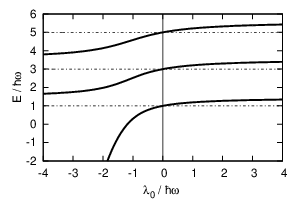
In this section we present the energy spectrum (in the center of mass frame) of two trapped particles interacting via a Gaussian-shaped potential in 2D, which results from Eq.(17). From now on we fix the harmonic oscillator length to . We first set and explore the dependence of the energy levels on the parameter . The energies of the first three states versus are plotted in Fig.(2). For the energies are always above the respective non-interacting values and the system is repulsive. As expected, at we recover the non-interacting values , which correspond to the poles of the left-hand side (lhs) of Eq.(17). For the particles are interacting attractively and the ground state energy quickly diverges to for .
The Gaussian-shaped two-body potential also allows us to study the role of the range, , of the interaction. In Fig.(3) we show the dependence of the ground-state energy on for three different values of the parameter . For repulsive interactions, i.e., , we find that with decreasing the ground-state energy logarithmically approaches the non-interacting value . This is in agreement with our discussion of the 2D delta potential in section III. We note that this behavior is also in agreement with the formal result in [31], where it is proven that in two and more dimensions the solutions of the Schrödinger equation are not affected by positive potentials with vanishing support. For attractive interactions () the dependence on is more pronounced and we observe that in the limit the energy of the ground state diverges to for any negative . This result is also consistent with previous studies, where it was observed that the attractive (non-regularized) delta potential yields a bound state with an infinitely negative energy. This is, in fact, the starting point for renormalization treatments [19, 32].

V Comparison with zero-range results
The energy spectrum of two harmonically trapped particles with a zero-range interaction in 2D has previously been obtained in the literature using a regularized delta potential [16], general scattering arguments [25], and modified boundary conditions [27]. In all three works the authors derive a transcendental equation for the energy, which can be written in the form
| (18) |
Here denotes the Digamma function, is the 2D scattering length, and is the harmonic oscillator length. The interaction strength is controlled through an interaction parameter defined as [16, 25]. The constant factor , which is slightly different within the works [16, 25, 27], depends on the exact form for the effective range expansion that the respective authors use (see the discussion at the end of [25]) and has no consequence on the following analysis.
In order to relate our finite-range result for the energy of two trapped interacting particles to the zero-range treatments, we employ a Taylor expansion of the lhs of Eq.(17) around [33]
| (19) |
Here is the Euler-Mascheroni constant and is again the Digamma function. By neglecting terms of order and after rearranging, we can rewrite Eq.(17) for as
| (20) |
with . Evidently, the above equation for the energy has the same form as the literature result in (18), and by an appropriate choice of and our ansatz reproduces the zero-range spectrum. By comparing the rhs of Eq.(20) and (18) we immediately see that (for weak interactions) the interaction parameter is equal to in our finite-range analysis [34]. Thus, the interaction parameter in 2D is proportional to the factor in front of the two-body potential [see Eq.(1)].
The Taylor expansion in (19) leads to two significant differences between the zero-range spectrum and the finite-range spectrum already presented in Fig.(2). First, when the interaction is repulsive, i.e., , Eq.(20) yields an additional deeply-bound state which is not present in the original finite-range spectrum (see also [35] for the case of hard spheres in three dimensions, where also a redundant state appears in the zero-range pseudopotential approximation). This state appears due to the different asymptotic behavior of both sides of (19) in the limit . While the lhs of (19) converges to 0, the expanded rhs diverges to , see Fig.(4). This also leads to a second difference. The finite-range result yields a bound state with an energy approaching for , while the zero-range equation yields a finite value which corresponds to the zero crossing appearing for negative in Fig.(2). This demonstrates that the short-ranged 2D Gaussian-shaped interaction potential and the zero-range potential approximate each other well except for the ground state.
Equating the rhs of Eq.(20) and (18) allows us to obtain a connection between the 2D scattering length, , and the parameters of the Gaussian-shaped potential and . Using from [25], and noticing that the authors use the definition of the harmonic oscillator length with the full mass, we obtain
| (21) |
for the 2D scattering length of a Gaussian-shaped potential of width . We find good quantitative agreement when we compare the above expression for with numerical values from [36]. For and the relative difference between our analytical estimate and the numerical value is about one percent. Even in the regime of and , where the accuracy of our treatment is limited, the relative difference in only about 8 percent.

VI Summary
We analyzed the problem of two harmonically trapped particles in 2D, which interact via a finite-ranged Gaussian-shaped two-body potential. We derived an approximative transcendental equation for the energy which is demonstrated to be highly accurate for the ground state. Moreover, our ansatz works well also for the excited states (see Appendix D). Using the Gaussian-shaped potential we were able to directly study the dependence of the ground-state energy on the range of the interaction. We found that the effect of the short-ranged interaction on the ground-state energy vanishes logarithmically with deceasing of the potential range, , for all positive interaction strengths. This study is complemented by a variational treatment which shows that in the limit of a (non-regularized) delta potential, i.e. , the energy spectrum of the two (repelling) particles can be made arbitrarily close to the respective non-interacting one by increasing the size of the Hilbert space. Finally, we established and discussed the connection between our finite-range result and earlier zero-range treatments reported in the literature.
Our analysis shows that a Gaussian-shaped two-body potential and its zero-range pseudopotential give similar results for both repulsive and attractive interactions except for the lowest eigenstate of the latter. Here, for repulsion the zero-range pseudopotential leads to an additional dimer bound state which is not connected to the unperturbed system when the interaction is switched off. Consequently, this dimer state is difficult to reach when the interaction is smoothly switched on. When going beyond two particles, analytical treatments quickly become inaccessible, leaving one only with a numerical recourse. For the numerical many-body simulations one usually prefers to use smooth, finite-ranged, model interaction potentials. Our results support the applicability of the Gaussian-shaped potential as a model of the two-body interaction in such simulations in two dimensions, see for example [36].
Acknowledgements.
We thank Axel Lode and Kaspar Sakmann for very helpful discussions. Financial support by the Deutsche Forschungsgemeinschaft (DFG) also within the framework of the Enable fund of the excellence initiative at Heidelberg university is acknowledged.References
- [1] D. J. Bishop and J. D. Reppy, Phys. Rev. Lett. 40, 1727 (1978).
- [2] P. Minnhagen, Rev. Mod. Phys. 59, 1001 (1987).
- [3] M.-C. Cha, M. P. A. Fisher, S. M. Girvin, M. Wallin, and A. P. Young, Phys. Rev. B 44, 6883 (1991).
- [4] G. T. Seidler, T. F. Rosenbaum, and B. W. Veal, Phys. Rev. B 45, 10162 (1992).
- [5] N. Marković, C. Christiansen, A. M. Mack, W. H. Huber, and A. M. Goldman, Phys. Rev. B 60, 4320 (1999).
- [6] K. S. Novoselov, Rev. Mod. Phys. 83, 837 (2011).
- [7] S. Das Sarma, S. Adam, E. H. Hwang, and E. Rossi, Rev. Mod. Phys. 83, 407 (2011).
- [8] D. S. Petrov, D. M. Gangardt, and G. V. Shlyapnikov, J. Phys. IV 116, 5 (2004).
- [9] A. Görlitz, J. M. Vogels, A. E. Leanhardt, C. Raman, T. L. Gustavson, J. R. Abo-Shaeer, A. P. Chikkatur, S. Gupta, S. Inouye, T. Rosenband, et al., Phys. Rev. Lett. 87, 130402 (2001).
- [10] S. Burger, F. S. Cataliotti, C. Fort, P. Maddaloni, F. Minardi, and M. Inguscio, Europhys. Lett. 57, 1 (2002).
- [11] D. Rychtarik, B. Engeser, H.-C. Nägerl, and R. Grimm, Phys. Rev. Lett. 92, 173003 (2004).
- [12] Z. Hadzibabic, S. Stock, B. Battelier, V. Bretin, and J. Dalibard, Phys. Rev. Lett. 93, 180403 (2004).
- [13] N. L. Smith, W. H. Heathcote, G. Hechenblaikner, E. Nugent, and C. J. Foot, J. Phys. B 38, 223 (2005).
- [14] K. Martiyanov, V. Makhalov, and A. Turlapov, Phys. Rev. Lett. 105, 030404 (2010).
- [15] R. Jackiw, Diverse Topics in Theoretical and Mathematical Physics (World Scientific, Singapore, 1995).
- [16] T. Busch, B.-G. Englert, K. Rza̧żewski, and M. Wilkens, Found. Phys. 28, 549 (1998).
- [17] L. R. Mead and J. Godines, Am. J. Phys. 59, 935 (1991).
- [18] R. M. Cavalcanti, Revista Brasilleira de Ensino de Fisica 21, 336 (1998).
- [19] S.-L. Neyo, Am. J. Phys. 68, 571 (1999).
- [20] A. Sütő, J. Stat. Phys. 109, 1051 (2002).
- [21] B. D. Esry and C. H. Greene, Phys. Rev. A 60, 1451 (1999).
- [22] V. S. Araujo, F. A. B. Coutinho, and J. F. Perez, Am. J. Phys. 72, 203 (2004).
- [23] S. Albeverio, F. Gesztesy, R. Hoegn-Krohn, and H. Holden, Solvable Models in Quantum Mechanics (AMS Chelsea, Providence, 2004).
- [24] K. Wódkiewicz, Phys. Rev. A 43, 68 (1991).
- [25] A. Farrell and B. P. van Zyl, J. Phys. A 43, 015302 (2010).
- [26] T. K. Lim and P. A. Maurone, Phys. Rev. B 22, 1467 (1980).
- [27] X.-J. Liu, H. Hu, and P. D. Drummond, Phys. Rev. B 82, 054524 (2010).
- [28] M. Abramowitz and A. Stegun, eds., Handbook of Mathematical Functions (Dover, New York, 1972).
- [29] M. L. Boas, Mathematical Methods in the Physical Sciences (John Wiley and Sons, New York, 1983).
- [30] W. Magnus, F. Oberhettinger, and F. G. Tricomy, Higher Transcendental Functions (McGraw Hill, New York, 1953).
- [31] C. N. Friedman, J. Funct. Anal. 10, 346 (1972).
- [32] H. Lee, H. Hsu, and L. E. Reichl, Phys. Rev. B 71, 045307 (2005).
- [33] S. Wolfram, Mathematica 8 (Wolfram Research Inc., Champaign, IL, 2011).
- [34] We can also obtain this directly by substituting (21) in and expanding for small , which leads to .
- [35] M. Block and M. Holthaus, Phys. Rev. A 65, 052102 (2002).
- [36] J. Christensson, C. Forssén, S. Åberg, and S. M. Reimann, Phys. Rev. A 79, 012707 (2009).
- [37] S. Flügge, Practical Quantum Mechanics I, vol. 1 (Springer, Berlin, 1971).
Appendix A Evaluation of the matrix elements
Here we outline the calculation of the matrix elements in Eq.(7) of the main text. The radial part of the zero angular momentum eigenfunctions of the 2D harmonic oscillator can be written in terms of the Laguerre polynomials . With the eigenstates read [37]
| (22) |
We need to evaluate the integral
| (23) |
We start by setting and rewriting
| (24) |
Now we define a new variable and obtain
| (25) |
To get rid of the factor in the argument of we use the known multiplication formula for Laguerre polynomials [28]
| (26) |
By substituting the above expression for and into the integral of Eq.(25), and by making use of the orthogonality of the Laguerre polynomials with respect to the weight function , we obtain
| (27) |
We can write the above expression as
| (28) |
In order to express the sum in terms of the Gauss hypergeometric function , we rewrite the above expression using the Pochhammer symbols for the rising factorial [28]
| (29) |
We can now directly use the definition of [28] and obtain
| (30) |
Finally, by changing back to the original variables, we arrive at Eq.(7) of the main text.
Appendix B Variational energy
Here we show that the approach in Section II A for the energy spectrum of the non-regularized delta potential is essentially a variational treatment with and . For this purpose, let us consider just as a parameter which fulfills Eq.(11) for a given and fixed finite . The variational energy then reads
| (31) |
We thus see that the variational energy is indeed equal to . In the last step we used the normalization condition for the wavefunction .
Appendix C Ansatz for in the finite-range case
Here we discuss the ansatz for the expansion coefficients in Eq.(13). We stress that the approach is general. Let us consider a Hamilton operator
| (32) |
and assume that the eigenstates and eigenenergies of are known. We denote them by with . For an eigenstate of the full Hamilton operator we can write
or equivalently
| (33) |
After projection on an unperturbed state we express the above equation in the form
| (34) |
From here we obtain a symbolic expression for the expansion coefficients
| (35) |
Until now we have not used any approximations. Of course, the above expression is only an implicit one, because the unknown state , which is itself dependent on , appears on the rhs. Our ansatz in Eq.(13) of the main text consists in taking only a “first-order approximation” for the expansion coefficients, i.e. we substitute in (35) and obtain
| (36) |
Of course, we can also substitute into Eq.(36) and obtain similar expressions which might be more efficient when studying excited states.
Appendix D Numerical comparison
In this section we compare energies obtained by solving Eq.(17) with the numerical values determined by the full direct diagonalization of the Hamiltonian using the matrix elements in Eq.(7). In Tab.(1) we show the relative difference between both values, i.e. , where denotes the value obtained from direct diagonalization and denotes the energy obtained by solving Eq.(17). The comparison is performed for the ground state (GS) and several excited states with zero angular momentum [see the first column in Tab.(1)]. We observe an excellent agreement between the values from both methods, with in the order of and below, see Tab.(1).
We also perform a study for a fixed width, , and variable . The results are shown in Fig.(5), where we plot the values of the ground-state energy as obtained from Eq.(17) and direct diagonalization. The values obtained from Eq.(17) are in excellent agreement with the ones from direct diagonalization for up to . Analogous behavior was also found for the excited states.
| GS | ||||
|---|---|---|---|---|
| 1st | ||||
| 2nd | ||||
| 4th | ||||
| 8th | ||||
| 16th |
