QCD Phase Diagram with 2-flavor Lattice Fermion FormulationsThanks: RIKEN-MP-57

Lattice QCD has played an important role in study of the non-perturbative aspects of QCD. However, its application to the finite density system has not been established due to serious difficulty of the sign problem. In this report we propose a new framework of investigating the 2-flavor QCD with finite temperature and density by using the Karsten-Wilczek (KW) lattice fermion [1], which possesses only two species doublers, i.e. minimally doubled fermion. This lattice formulation lifts degeneracy of 16 species without breaking its chiral symmetry by introducing a species-dependent imaginary chemical potential, instead of a species-dependent mass term introduced in the Wilson fermion formalism. Because of the chemical potential term, its discrete symmetry is not sufficient to be applied to fully Lorentz symmetric system, i.e. zero temperature and density, but enough to study the in-medium QCD. To show the usefulness of the KW fermion, we study strong-coupling lattice QCD with temperature and density.

The KW fermion is a kind of minimally doubled fermions, involving only two species doublers by introducing a species-dependent imaginary chemical potential, which we call “flavored chemical potential”. This term preserves its chiral symmetry and ultra-locality [2], but breaks some of discrete spacetime symmetries [3, 4]. We then need three counter terms to take a correct Lorentz symmetric continuum limit: dimension-3, $\bar{\psi}i\gamma_{4}\psi=i\psi^{\dagger}\psi$, and dimension-4 terms, $\bar{\psi}\gamma_{4}\partial_{4}\psi$, $F_{j4}F_{j4}$ [5]. The fermionic part of KW fermion action with the counter terms is given by

The second term in the first line including $i\gamma_{4}$ is the flavored chemical potential term, which we also call Karsten-Wilczek(KW) term. We here introduce a parameter $r$ in analogy to Wilson fermion. $\mu_{3}$ and $d_{4}$ are parameters for the dimension-3 and dimension-4 counter terms, respectively. The corresponding Dirac operator in the momentum space yields

which has only two zeros at $\bar{p}=(0,0,0,\frac{1}{a}\mathrm{arcsin}\left(-\frac{\mu_{3}}{1+d_{4}}\right))$ when $-1-d_{4}<\mu_{3}<1+d_{4}$ with $r=1$. When we expand the Dirac operator around the zeros, its dispersion relation is not Lorentz symmetric. As shown in Ref.[2], the tuning condition for the correct dispersion relation is given by $(1+d_{4})^{2}=1+\mu_{3}^{2}$ at the tree level. Moreover, it is shown that $\mu_{3}$ has to be tuned to control imaginary chemical potential in $\mathcal{O}(1/a)$.

Symmetries of the lattice action (1) are chiral symmetry, cubic symmetry corresponding to permutation of spatial three axes, CT and P [3]:

1. 1.

   $\mathrm{U}\,(1)$ chiral symmetry ($\gamma_{5}\otimes\tau_{3}$ [6, 7, 8])

2. 2.

   Cubic symmetry

3. 3.

   CT

4. 4.

   P

It is notable that these symmetries are the same as those of the finite-density lattice QCD: As an example, we look into the naive lattice action with chemical potential, which is given by

The 4th direction hopping term, involving chemical potential, breaks the hypercubic symmetry into the spatial cubic symmetry, and also C, P, and T into CT and P, which are the same symmetries of (1). It means that, even if we introduce chemical potential as (3) to KW fermion, the symmetries are unchanged. The KW fermion with the exponential form chemical potential is given by,

From the viewpoint of the universality class, these two theories, (3) and (4), should belong to the same class.

Here we remark the way of introducing chemical potential. It was pointed out in [9] that a naive form of the chemical potential, $\mu\psi^{\dagger}\psi=\mu\bar{\psi}\gamma_{4}\psi$, violates the Abelian gauge invariance and requires a counter term to make thermodynamical quantities finite. On the other hand, in the KW fermion, the flavored chemical potential term is introduced in this naive form. It leads to necessity of tuning $\mu_{3}$ to deal with $\mathcal{O}(1/a)$ additive renormalization of chemical potential, as with the mass renormalization in the Wilson fermion. This renormalization effect is relevant to the phase diagram in the $(\mu_{3}$-$g^{2})$ parameter plane, as discussed in [2].

We study QCD phase diagram in the framework of the strong-coupling lattice QCD with KW-type minimally doubled fermion. We extend the strong-coupling analysis with this lattice fermion [10] to the finite temperature and density system [11, 12, 13]. The effective potential in terms of the meson field is obtained by performing the 1-link integral in the strong coupling limit $(g^{2}\to\infty)$, and then introducing auxiliary fields to eliminate the 4-point interactions. In the case with KW fermion, we have to consider both of the scalar $\sigma=\langle\bar{\psi}\psi\rangle$ and vector $\pi_{4}=\langle\bar{\psi}i\gamma_{4}\psi\rangle$ condensates. Identifying $\bar{\psi}\gamma_{4}=\psi^{\dagger}$, the latter corresponds to the imaginary density $i\langle\psi^{\dagger}\psi\rangle$. For the case with $\mathrm{SU}\,(N_{c})$ gauge group and $d=D+1$ dimensions in the finite temperature and density, we obtain the the following effective potential,

In particular, the determinant part for $N_{c}=3$ is given by

with

Here the baryon chemical potential is defined as $\mu_{B}=3\mu$. Remark that the next-leading order terms in $\mathcal{O}(1/\sqrt{D})$ are omitted in the derivation. See [14] for the detailed calculation.

In the zero temperature case, we can solve the equilibrium condition analytically. For $D=3$ ($d=4$) with $m=0$ and $r=1$ the potential is given by

In this case there are two local minima of the free energy as a function of $\sigma$ at $\sigma=0$ and $\sigma=\sigma_{0}$. This $\sigma_{0}$ can be determined by the gap equation, $\partial\mathcal{F}_{\rm eff}/\partial\sigma\Big|_{\sigma=\sigma_{0}}=0$,

Comparing these two local minima, we can show that the global minimum changes from $\sigma=\sigma_{0}$ to $\sigma=0$ at the critical chemical potential as

This chiral phase transition is of 1st order because the order parameter $\sigma$ changes discontinuously at this critical chemical potential. We can also evaluate the baryon density $\rho_{B}=-\partial\mathcal{F}_{\rm eff}/\partial\mu_{B}$ at $T=0$. It turns out to be empty $\rho_{B}=0$ when $\mu_{B}<\mu_{B}^{\rm critical}$. On the other hand, when $\mu_{B}>\mu_{B}^{\rm critical}$, it is saturated as $\rho_{B}=1$.

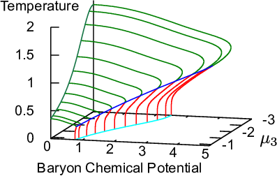
We then discuss the phase diagram with respect to chiral symmetry. We now concentrate on the case with $r=1$ for simplicity because the effective potential (5) is independent of $\pi_{4}$ in such a case. The 2nd order chiral phase boundary is given by the condition, such that the coefficient of $\sigma^{2}$ in the effective potential (5) becomes zero. When the order of the phase transition is changed from 2nd to 1st, the coefficient of $\sigma^{4}$ as well as $\sigma^{2}$ should vanish. The left panel of Fig. 1 shows the phase boundary of the chiral transition with $r=1$, $\mu_{3}=-0.9$ and $m=0$ for $d_{4}=0$. The counter term parameter is taken from the physical region $-\sqrt{32/7}<\mu_{3}+3<\sqrt{32/7}$ [2]. The order of the phase transition is changed from 2nd to 1st at the tricritical point $(\mu_{B}^{\rm tri},T^{\rm tri})=(0.804,0.234)$. We also depict $\sigma$ condensate and the baryon density $\rho_{B}=-\partial\mathcal{F}_{\rm eff}/\partial\mu_{B}$ as functions of $\mu_{B}$ with several fixed $T$ in Fig. 2. We find that there are 1st ($T<T^{\mathrm{tri}}$) and 2nd ($T>T^{\mathrm{tri}}$) order phase transitions for $\sigma$, followed by the phase transition of the density $\rho_{B}$. For $m\not=0$, we can show that the crossover transition instead appears with the 2nd order critical point.

These results are qualitatively consistent with those with strong-coupling lattice QCD with staggered fermions, while there are some quantitative differences. For example, the KW phase diagram is suppressed in $T$ direction compared to that in staggered. We here compare the ratio of the transition baryon chemical potential at $T=0$ to the critical temperature at $\mu_{B}=0$, $R^{0}=\mu_{c}(T=0)/T_{c}(\mu_{B}=0)$. In staggered fermion, this ratio is $R^{0}_{\mathrm{st}}\simeq 3\times 0.56/(5/3)\sim 1$ [12, 13], while $R^{0}_{\mathrm{KW}}\simeq 0.767/0.356\sim 2.2$. In the real world, this ratio is larger, $R^{0}\gtrsim M_{N}/170~\mathrm{MeV}\sim 5.5$. When the finite coupling and Polyakov loop effects are taken into account for staggered fermion, $T_{c}(\mu_{B}=0)$ decreases, $\mu_{c}(T=0)$ stays almost constant, then $R^{0}$ value increases [15]. Larger $R^{0}$ with KW fermion in the strong coupling limit may suggest smaller finite coupling corrections in the phase boundary. Another interesting point is the location of the tricritical point. In KW fermion, the ratio is $R^{\mathrm{tri}}_{\mathrm{KW}}=0.804/0.234\simeq 3.4$, while $R^{\mathrm{tri}}_{\mathrm{st}}=1.73/0.866\simeq 2.0$ for unrooted staggered fermion [12, 13]. It would be too brave to discuss this value, but $R^{\mathrm{tri}}_{\mathrm{KW}}$ is consistent with the recent Monte-Carlo simulations (see references in [16]), which implies that the critical point does not exist in the low baryon chemical potential region, $\mu_{B}/T\lesssim 3$. These observations reveal usefulness of KW fermion for research on QCD phase diagram.

Apart from the phase transitions, the $\mu_{B}$ dependence of $\sigma$ and $\rho_{B}$ seems to have some characteristics in Fig. 2. At $T=0.3>T^{\mathrm{tri}}$ with m=0, $\sigma$ and $\rho_{B}$ undergoes the 2nd-order phase transition at $\mu_{B}\simeq 0.5$, and at a larger $\mu_{B}$ ($\mu_{B}\simeq 1.15$), increasing rate of $\rho_{B}$ as a function of $\mu_{B}$ becomes higher again. At lower temperature, $T=0.2<T^{\mathrm{tri}}$, partial restoration of the chiral symmetry is seen before the first order phase transition. Since we have not taken care of the diquark condensate, these continuous changes are not related to the color superconductor. Other types of matter, such as quarkyonic matter [17], partial chiral restored matter [15], or nuclear matter, may be related to the above characteristics.

In this report we focus on the case with $r=1$ and $d_{4}=0$ for simplicity. It is shown in [14] that effects of these parameters are just quantitative.

We have proposed a new framework for investigating the two-flavor finite-($T$,$\mu$) QCD phase diagram. We have shown that the discrete symmetries of KW fermion strongly suggest its applicability to the in-medium lattice QCD. To support our idea, we study the strong-coupling lattice QCD in the medium and derive the phase diagram of chiral symmetry for finite temperature and chemical potential. We have obtained the phase diagram with 1st, 2nd-order and crossover critical lines, which is qualitatively in agreement to results from the model study.

References

- [1] L. H. Karsten, Phys. Lett. B104 (1981) 315; F. Wilczek, Phys. Rev. Lett. 59 (1987) 2397.
- [2] T. Misumi, JHEP 1208 (2012) 068, arXiv:1206.0969 [hep-lat].
- [3] P. F. Bedaque, M. I. Buchoff, B. C. Tiburzi, and A. Walker-Loud, Phys. Lett. B662 (2008) 449, arXiv:0801.3361 [hep-lat]; Phys. Rev. D78 (2008) 017502, arXiv:0804.1145 [hep-lat].
- [4] T. Kimura and T. Misumi, Prog. Theor. Phys. 124 (2010) 415–432, arXiv:0907.1371 [hep-lat]; Prog. Theor. Phys. 123 (2010) 63–78, arXiv:0907.3774 [hep-lat].
- [5] S. Capitani, J. Weber, and H. Wittig, Phys. Lett. B681 (2009) 105, arXiv:0907.2825 [hep-lat]; S. Capitani, M. Creutz, J. Weber, and H. Wittig, JHEP 09 (2010) 027, arXiv:1006.2009 [hep-lat].
- [6] M. Creutz, T. Kimura, and T. Misumi, JHEP 12 (2010) 041, arXiv:1011.0761 [hep-lat].
- [7] B. C. Tiburzi, Phys. Rev. D82 (2010) 034511, arXiv:1006.0172 [hep-lat].
- [8] L. Drissi, E. Saidi, and M. Bousmina, J. Math. Phys. 52 (2011) 022306, arXiv:1101.1061 [hep-lat]; L. B. Drissi and E. H. Saidi, Phys. Rev. D84 (2011) 014509, arXiv:1103.1316 [hep-lat].
- [9] P. Hasenfratz and F. Karsch, Phys. Lett. B125 (1983) 308.
- [10] T. Kimura, S. Komatsu, T. Misumi, T. Noumi, S. Torii, and S. Aoki, JHEP 01 (2012) 048, arXiv:1111.0402 [hep-lat].
- [11] Y. Nishida, K. Fukushima, and T. Hatsuda, Phys. Rept. 398 (2004) 281–300, arXiv:hep-ph/0306066 [hep-ph].
- [12] K. Fukushima, Prog. Theor. Phys. Suppl. 153 (2004) 204–219, arXiv:hep-ph/0312057 [hep-ph].
- [13] Y. Nishida, Phys. Rev. D69 (2004) 094501, arXiv:hep-ph/0312371.
- [14] T. Misumi, T. Kimura, and A. Ohnishi, arXiv:1206.1977 [hep-lat].
- [15] K. Miura, T. Z. Nakano, A. Ohnishi, and N. Kawamoto, Phys. Rev. D80 (2009) 074034, arXiv:0907.4245 [hep-lat]; K. Miura, T. Z. Nakano, and A. Ohnishi, Prog. Theor. Phys. 122 (2009) 1045–1054, arXiv:0806.3357 [nucl-th]; T. Z. Nakano, K. Miura, and A. Ohnishi, Prog. Theor. Phys. 123 (2010) 825–851, arXiv:0911.3453 [hep-lat].
- [16] A. Ohnishi, Prog. Theor. Phys. Suppl. 193 (2012) 1–10, arXiv:1112.3210 [nucl-th].
- [17] L. McLerran and R. D. Pisarski, Nucl. Phys. A796 (2007) 83–100, arXiv:0706.2191 [hep-ph].