Maximum likelihood estimator consistency for ballistic random walk in a parametric random environment.

Francis Comets Note: Laboratoire Probabilités et Modèles Aléatoires, Université Paris Diderot, UMR CNRS 7599, E-mail: comets@math.univ-paris-diderot.fr; $ˆ†$ Laboratoire Statistique et Génome, Université d’Évry Val d’Essonne, UMR CNRS 8071, USC INRA, E-mail: ${$mikael.falconnet, catherine.matias$}$@genopole.cnrs.fr; $ˆ‡$ Département Informatique, IUT de Fontainebleau, E-mail: oleg.loukianov@u-pec.fr; ^§ Laboratoire Analyse et Probabilités, Université d’Évry Val d’Essonne, E-mail: dasha.loukianova@univ-evry.fr Mikael Falconnet Oleg Loukianov Dasha Loukianova^§ Catherine Matias

Abstract

We consider a one dimensional ballistic random walk evolving in an i.i.d. parametric random environment. We provide a maximum likelihood estimation procedure of the parameters based on a single observation of the path till the time it reaches a distant site, and prove that the estimator is consistent as the distant site tends to infinity. We also explore the numerical performances of our estimation procedure.

Key words : Ballistic regime, maximum likelihood estimation, random walk in random environment. MSC 2000 : Primary 62M05, 62F12; secondary 60J25.

1 Introduction

Random walks in random environments (RWRE) have attracted much attention lately, mostly in the physics and probability theory literature. These processes were introduced originally by Chernov (1967) to model the replication of a DNA sequence. The idea underlying Chernov’s model is that the protein that moves along the DNA strand during replication performs a random walk whose transition probabilities depend on the sequence letters, thus modeled as a random environment. Since then, RWRE have been developed far beyond this original motivation, resulting into a wealth of fine probabilistic results. Some recent surveys on the subject include Hughes (1996) and Zeitouni (2004).

Recently, these models have regained interest from biophysics, as they fit the description of some physical experiments that unzip the double strand of a DNA molecule. More precisely, some fifteen years ago, the first experiments on unzipping a DNA sequence have been conducted, relying on several different techniques (see Baldazzi et al., 2006; Baldazzi et al., 2007, and the references therein). By that time, these experiments primarily took place in the quest for alternative (cheaper,faster or both) sequencing methods. When conducted in the presence of bounding proteins, such experiments also enabled the identification of specific locations at which proteins and enzymes bind to the DNA (Koch et al., 2002). Nowadays, similar experiments are conducted in order to investigate molecular free energy landscapes with unprecedented accuracy (Alemany et al., 2012; Huguet et al., 2009). Among other biophysical applications, one can mention the study of the formation of DNA or RNA hairpins (Bizarro et al., 2012).

Despite the emergence of data that is naturally modeled by RWRE, it appears that very few statistical issues on those processes have been studied so far. Very recently, Andreoletti and Diel (2012) considered a problem inspired by an experiment on DNA unzipping (Baldazzi et al., 2006; Baldazzi et al., 2007; Cocco and Monasson, 2008), where the aim is to predict the sequence of bases relying on the observation of several unzipping of one finite length DNA sequence. Up to some approximations, the problem boils down to considering independent and identically distributed (i.i.d.) replicates of a one dimensional nearest neighbour path (i.e. the walk has $\pm 1$ increments) in the same finite and two-sites dependent environment, up to the time each path reaches some value $M$ (the sequence length). In this setup, the authors consider both a discrete time and a continuous time model. They provide estimates of the values of the environment at each site, which corresponds to estimating the sequence letters of the DNA molecule. Moreover, they obtain explicit formula for the probability to be wrong for a given estimator, thus evaluating the quality of the prediction.

In the present work, we study a different problem, also motivated by some DNA unzipping experiments: relying on an arbitrary long trajectory of a transient one-dimensional nearest neighbour path, we would like to estimate the parameters of the environment’s distribution. Our motivation comes more precisely from the most recent experiments, that aim at characterising free binding energies between base pairs relying on the unzipping of a synthetic DNA sequence (Ribezzi-Crivellari et al., 2011). In this setup, the environment is still considered as random as those free energies are unknown and need to be estimated. While our asymptotic setup is still far from corresponding to the reality of those experiments, our work might give some insights on statistical properties of estimates of those binding free energies.

The parametric estimation of the environment distribution has already been studied in Adelman and Enriquez (2004). In their work, the authors consider a very general RWRE and provide equations relying the distribution of some statistics of the trajectory to some moments of the environment distribution. In the specific case of a one-dimensional nearest neighbour path, those equations give moment estimators for the environment distribution parameters. It is worth mentioning that due to its great generality, the method is hard to understand at first, but it takes a simpler form when one considers the specific case of a one-dimensional nearest-neighbour path. Now, the method has two main drawbacks: first, it is not generic in the sense that it has to be designed differently for each parametric setup that is considered. Namely, the method relies on the choice of a one-to-one mapping between the parameters and some moments. Note that the injectivity of such a mapping might even not be simple to establish (see for instance the case of Example II below, further developed in Section 5.1). Second, from a statistical point of view, it is clear that some mappings will give better results than others. Thus the specific choice of a mapping has an impact on the estimator’s performances.

As an alternative, we propose here to consider maximum likelihood estimation of the parameters of the environment distribution. We consider a transient nearest neighbour path in a random environment, for which we are able to define some criterion - that we call a log-likelihood of the observed process, see (8) below. Our estimator is then defined as the maximiser of this criterion - thus a maximum likelihood estimator. When properly normalised, we prove that this criterion is convergent as the size of the path increases to infinity. This part of our work relies on using the link between RWRE and branching processes in random environments (BPRE). While this link is already well-known in the literature, we provide an explicit characterisation of the limiting distribution of the BPRE that corresponds to our RWRE (see theorem 4.5 below). Relying on this precise characterisation, we then further prove that the limit of our normalised criterion is finite in what is called the ballistic region, namely the set of parameters such that the path has a linear increase (see Section 2.1 below for more details). Then, following standard statistical results, we are able to establish the consistency of our estimator. We also provide synthetic experiments to compare the effective performances of our estimator and Adelman and Enriquez’s procedure. In the cases where Adelman and Enriquez’s estimator is easily settled, while the two methods exhibit the same performances with respect to their bias, our estimator exhibits a much smaller variance. We mention that establishing asymptotic normality of this estimator requires much more technicalities and is out of the scope of the present work. This point will be studied in a companion article, together with variance estimates and confidence intervals.

The article is organised as follows. Section 2.1 introduces our setup: the one dimensional nearest neighbour path, and recalls some well-known results about the behaviour of those processes. Then in Section 2.2, we present the construction of our M-estimator (i.e. an estimator maximising some criterion function), state the assumptions required on the model as well as our consistency result (Section 2.3). Section 3 presents some examples of environment distributions for which the model assumptions are satisfied so that our estimator is consistent. Now, the proof of our consistency result is presented in Section 4. The section starts by recalling the link between RWRE and BPRE (Section 4.1). Then, we state our core result: the explicit characterisation of the limiting distribution of the branching process that is linked with our path; and its corollary: the existence of a (possibly infinite) limit for the normalised criterion (Section 4.2). In Section 4.3 we first provide a technical result on the uniformity of this convergence, then establish that in the ballistic case, the limit of the normalised criterion is finite. An almost converse statement is also given (Lemma 4.9). To conclude this part, we prove in Section 4.4 that the limiting criterion identifies the true parameter value (under a natural identifiability assumption on the model parameter). Finally, numerical experiments are presented in Section 5.2, focusing on the three examples that were developed in Section 3. Note that we also provide an explicit description of the form of Adelman and Enriquez’s estimator in the particular case of the one-dimensional nearest neighbour path in Section 5.1.

2 Definitions, assumptions and results

2.1 Random walk in random environment

Let $\omega=\{\omega_{x}\}_{x\in\mathbb{Z}}$ be an independent and identically distributed (i.i.d.) collection of $(0,1)$ -valued random variables with distribution $\nu$ . The process $\omega$ represents a random environment in which the random walk will evolve. We suppose that the law $\nu=\nu_{\theta}$ depends on some unknown parameter $\theta\in\Theta,$ where $\Theta\subset\mathbb{R}^{d}$ is assumed to be a compact set. Denote by $\mathbb{P}^{\theta}=\nu_{\theta}^{\otimes\mathbb{Z}}$ the law on $(0,1)^{\mathbb{Z}}$ of the environment $\{\omega_{x}\}_{x\in\mathbb{Z}}$ and by $\mathbb{E}^{\theta}$ the expectation under this law.

For fixed environment $\omega$ , let $X=\{X_{t}\}_{t\in\mathbb{N}}$ be the Markov chain on $\mathbb{Z}$ starting at $X_{0}=0$ and with transition probabilities

P_{\omega}(X_{t+1}=y|X_{t}=x)=\left\{\begin{array}[]{lr}\omega_{x}&\mbox{if}\ y=x+1,\\ 1-\omega_{x}&\mbox{if}\ y=x-1,\\ 0&\mbox{otherwise}.\end{array}\right.

The symbol $P_{\omega}$ denotes the measure on the path space of $X$ given $\omega$ , usually called quenched law. The (unconditional) law of $X$ is given by

\mathbf{P}^{\theta}(\cdot)=\int P_{\omega}(\cdot)\mathrm{d}\mathbb{P}^{\theta}(\omega),

this is the so-called annealed law. We write $E_{\omega}$ and $\mathbf{E}^{\theta}$ for the corresponding quenched and annealed expectations, respectively. We start to recall some well-known asymptotic results. Introduce a family of i.i.d. random variables,

\rho_{x}=\frac{1-\omega_{x}}{\omega_{x}},\qquad x\in{\mathbb{Z}},

(1)

and assume that $\log\rho_{0}$ is integrable. Solomon (1975) proved the following classification:

(a)

if $\mathbb{E}^{\theta}(\log\rho_{0})<0$ , then

$\displaystyle{\lim_{t\rightarrow\infty}X_{t}=+\infty},\quad\mathbf{P}^{\theta}\mbox{-almost surely}.$

(b)

If $\mathbb{E}^{\theta}(\log\rho_{0})=0$ , then

\displaystyle{-\infty=\liminf_{t\rightarrow\infty}X_{t}<\limsup_{t\rightarrow\infty}X_{t}=+\infty},\quad\mathbf{P}^{\theta}\mbox{-almost surely}.

The case of $\mathbb{E}^{\theta}(\log\rho_{0})>0$ follows from (a) by changing the sign of $X$ . Note that the walk $X$ is $\mathbf{P}^{\theta}$ -almost surely transient in case (a) and recurrent in case (b).

In the present paper, we restrict to the case (a) when $X$ is transient to the right. Then, it was also found that the rate of its increase (with respect to time $t$ ) is either linear or slower than linear. The first case is called ballistic case and the second one sub-ballistic case. More precisely, letting $T_{n}$ be the first hitting time of the positive integer $n$ ,

T_{n}=\inf\{t\in\mathbb{N}\,:\,X_{t}=n\},

(2)

and assuming $\mathbb{E}^{\theta}(\log\rho_{0})<0$ all through, we have

(a1)

if $\mathbb{E}^{\theta}(\rho_{0})<1$ , then, $\mathbf{P}^{\theta}\mbox{-almost surely},$

$\frac{T_{n}}{n}\xrightarrow[n\rightarrow\infty]{}\frac{1+\mathbb{E}^{\theta}(\rho_{0})}{1-\mathbb{E}^{\theta}(\rho_{0})},$ (3)
(a2)

If $\mathbb{E}^{\theta}(\rho_{0})\geq 1$ , then $T_{n}/n\rightarrow+\infty$ $\mathbf{P}^{\theta}\mbox{-almost surely}$ , when $n$ tends to infinity.

2.2 Construction of a M-estimator

We address the following statistical problem: estimate the unknown parameter $\theta$ from a single observation of the RWRE path till the time it reaches a distant site. Assuming transience to the right, we then observe $X_{[0,T_{n}]}=\{X_{t}\,:\,t=0,1,\ldots,T_{n}\}$ , for some $n\geq 1$ .

If $\mathbf{x}_{[0,t]}:=(x_{0},\dots,x_{t})$ is a nearest neighbour path of length $t$ , we define for all $x\in\mathbb{Z},$

		$\displaystyle L(x,\mathbf{x}_{[0,t]}):=\sum_{s=0}^{t-1}\mathbf{1}\{x_{s}=x;\ x_{s+1}=x-1\},$		(4)
	and	$\displaystyle R(x,\mathbf{x}_{[0,t]}):=\sum_{s=0}^{t-1}\mathbf{1}\{x_{s}=x;\ x_{s+1}=x+1\},$		(5)

the number of left steps (resp. right steps) from site $x$ . (Here, $\mathbf{1}\{\cdot\}$ denotes the indicator function). We let also $v_{t}$ (resp. $V_{T_{n}}$ ) be the set of integers visited by the path $\mathbf{x}_{[0,t]}$ (resp. $X_{[0,T_{n}]}$ ). Consider now a nearest neighbour path $\mathbf{x}_{[0,t_{n}]}$ starting from 0 and first hitting site $n$ at time $t_{n}$ . It is straightforward to compute its quenched and annealed probabilities, respectively

P_{\omega}(X_{[0,T_{n}]}=\mathbf{x}_{[0,t_{n}]})=\prod_{x\in v_{t_{n}}}\omega^{R(x,\mathbf{x}_{[0,t_{n}]})}_{x}(1-\omega_{x})_{{\phantom{x}}}^{L(x,\mathbf{x}_{[0,t_{n}]})}

and

\mathbf{P}^{\theta}(X_{[0,t_{n}]}=\mathbf{x}_{[0,t_{n}]})=\prod_{x\in v_{t_{n}}}\int_{0}^{1}a^{R(x,\mathbf{x}_{[0,t_{n}]})}(1-a)^{L(x,\mathbf{x}_{[0,t_{n}]})}\mathrm{d}\nu_{\theta}(a).

Under the following assumption, these weights add up to 1 over all possible choices of $\mathbf{x}_{[0,t_{n}]}$ .

Assumption I.

(Transience to the right). For any $\theta\in\Theta$ , $\mathbb{E}^{\theta}|\log\rho_{0}|<\infty$ and

\mathbb{E}^{\theta}(\log\rho_{0})<0.

Introducing the short-hand notation

L_{x}^{n}:=L(x,X_{[0,T_{n}]})\quad\mbox{and}\quad R_{x}^{n}:=R(x,X_{[0,T_{n}]}),

we can express the (annealed) log-likelihood of the observations as

\tilde{\ell}_{n}(\theta)=\sum_{x=0}^{n-1}\log\int_{0}^{1}a^{R_{x}^{n}}(1-a)^{L_{x}^{n}}\mathrm{d}\nu_{\theta}(a)+\sum_{x<0,x\in V_{T_{n}}}\log\int_{0}^{1}a^{R_{x}^{n}}(1-a)^{L_{x}^{n}}\mathrm{d}\nu_{\theta}(a).

(6)

Note that as the random walk $X$ starts from $0$ (namely $X_{0}=0$ ) and is observed until the first hitting time $T_{n}$ of $n\geq 1$ , we have $R_{x}^{n}=L_{x+1}^{n}+1$ for $x=1,2,\ldots,n-1$ . We will perform this change in the first line of the right-hand side of (6). Also, since the walk is transient to the right (Assumption I), the second sum in the right-hand side (accounting for negative sites $x$ ) is almost surely bounded. Hence, this sum will not influence in a significant way the behaviour of the normalised log-likelihood, and we will drop it. Therefore, we are led to the following choice.

Definition 2.1.

Let $\phi_{\theta}$ be the function from $\mathbb{N}^{2}$ to $\mathbb{R}$ given by

\phi_{\theta}(x,y)=\log\int_{0}^{1}a^{x+1}(1-a)^{y}\mathrm{d}\nu_{\theta}(a).

(7)

The criterion function $\theta\mapsto\ell_{n}(\theta)$ is defined as

\ell_{n}(\theta)=\sum_{x=0}^{n-1}\phi_{\theta}(L_{x+1}^{n},L_{x}^{n}),

(8)

that is the first sum (dominant term) in (6).

We maximise this criterion function to obtain an estimator of the unknown parameter. To prove convergence of the estimator, some assumptions are further required.

Assumption II.

(Ballistic case). For any $\theta\in\Theta,\ \mathbb{E}^{\theta}(\rho_{0})<1$ .

As already mentioned, Assumption I is equivalent to the transience of the walk to the right, and together with Assumption II, it implies positive speed.

Assumption III.

(Continuity). For any $x,y\in\mathbb{N}$ , the map $\theta\mapsto\phi_{\theta}(x,y)$ is continuous on $\Theta$ .

Assumption III is equivalent to the map $\theta\mapsto\nu_{\theta}$ being continuous on $\Theta$ with respect to the weak topology.

Assumption IV.

(Identifiability). $\forall(\theta,\theta^{\prime})\in\Theta^{2},$ $\nu_{\theta}\neq\nu_{\theta^{\prime}}\iff\theta\neq\theta^{\prime}.$

Assumption V.

The collection of probability measures $\{\nu_{\theta}\,:\,\theta\in\Theta\}$ is such that

\inf_{\theta\in\Theta}\mathbb{E}^{\theta}[\log(1-\omega_{0})]>-\infty.

Note that under Assumption II we have $\mathbb{E}^{\theta}[\log\omega_{0}]>-\log 2$ for any $\theta\in\Theta$ . Assumptions III and V are technical and involved in the proof of the consistency of our estimator. Assumption IV states identifiability of the parameter $\theta$ with respect to the environment distribution $\nu_{\theta}$ and is necessary for estimation.

According to Assumption III, the function $\theta\mapsto\ell_{n}(\theta)$ is continuous on the compact parameter set $\Theta$ . Thus, it achieves its maximum, and we define the estimator $\widehat{\theta}_{n}$ as a maximiser.

Definition 2.2.

An estimator $\widehat{\theta}_{n}$ of $\theta$ is defined as a measurable choice

\widehat{\theta}_{n}\in\mathop{\rm Argmax}_{\theta\in\Theta}\ell_{n}(\theta).

(9)

Note that $\widehat{\theta}_{n}$ is not necessarily unique.

Remark 2.3.

The estimator $\widehat{\theta}_{n}$ is a $M$ -estimator, that is, the maximiser of some criterion function of the observations. The criterion $\ell_{n}$ is not exactly the log-likelihood for we neglected the contribution of the negative sites. However, with some abuse of notation, we call $\widehat{\theta}_{n}$ a maximum likelihood estimator.

2.3 Asymptotic consistency of the estimator in the ballistic case

From now on, we assume that the process $X$ is generated under the true parameter value ${\theta^{\star}}$ , an interior point of the parameter space $\Theta$ , that we want to estimate. We shorten to $\mathbf{P}^{\star}$ and $\mathbf{E}^{\star}$ (resp. $\mathbb{P}^{\star}$ and $\mathbb{E}^{\star}$ ) the annealed (resp. quenched) probability $\mathbf{P}^{{\theta^{\star}}}$ (resp. $\mathbb{P}^{{\theta^{\star}}}$ ) and corresponding expectation $\mathbf{E}^{{\theta^{\star}}}$ (resp. $\mathbb{E}^{\theta^{\star}}$ ) under parameter value ${\theta^{\star}}$ .

Theorem 2.4.

(Consistency). Under Assumptions I to V, for any choice of $\widehat{\theta}_{n}$ satisfying (9), we have

\lim_{n\rightarrow\infty}\widehat{\theta}_{n}={\theta^{\star}},

in $\mathbf{P}^{\star}$ -probability.

3 Examples

3.1 Environment with finite and known support

Example I.

Fix $a_{1}<a_{2}\in(0,1)$ and let $\nu=p\delta_{a_{1}}+(1-p)\delta_{a_{2}}$ , where $\delta_{a}$ is the Dirac mass located at $a$ . Here, the unknown parameter is the proportion $p\in\Theta\subset[0,1]$ (namely $\theta=p$ ). We suppose that $a_{1}$ , $a_{2}$ and $\Theta$ are such that Assumptions I and II are satisfied.

This example is easily generalised to $\nu$ having $m\geq 2$ support points namely $\nu=\sum_{i=1}^{m}p_{i}\delta_{a_{i}}$ , where $a_{1},\dots,a_{m}$ are distinct, fixed and known in $(0,1)$ , we let $p_{m}=1-\sum_{i=1}^{m-1}p_{i}$ and the parameter is now $\theta=(p_{1},\dots,p_{m-1})$ .

In the framework of Example I, we have

\phi_{p}(x,y)=\log[pa_{1}^{x+1}(1-a_{1})^{y}+(1-p)a_{2}^{x+1}(1-a_{2})^{y}],

(10)

and

\ell_{n}(p):=\ell_{n}(\theta)=\sum_{x=0}^{n-1}\log\Big[pa_{1}^{L_{x+1}^{n}+1}(1\!-\!a_{1})_{\phantom{1}}^{L_{x}^{n}}+(1\!-\!p)a_{2}^{L_{x+1}^{n}+1}(1\!-\!a_{2})_{\phantom{2}}^{L_{x}^{n}}\Big].

(11)

Now, it is easily seen that Assumptions III to V are satisfied. Coupling this point with the concavity of the function $p\mapsto\ell_{n}(p)$ implies that $\widehat{p}_{n}=\mathop{\rm Argmax}_{p\in\Theta}\ell_{n}(p)$ is well-defined and unique (as $\Theta$ is a compact set). There is no analytical expression for the value of $\widehat{p}_{n}$ . Nonetheless, this estimator may be easily computed by numerical methods. Finally, it is consistent from Theorem 2.4.

3.2 Environment with two unknown support points

Example II.

We let $\nu=p\delta_{a_{1}}+(1-p)\delta_{a_{2}}$ and now the unknown parameter is $\theta=(p,a_{1},a_{2})\in\Theta$ , where $\Theta$ is a compact subset of

(0,1)\times\{(a_{1},a_{2})\in(0,1)^{2}\,:\,a_{1}<a_{2}\}.

We suppose that $\Theta$ is such that Assumptions I and II are satisfied.

This case is particularly interesting as it corresponds to one of the setups in the DNA unzipping experiments, namely estimating binding energies with two types of interactions: weak or strong.

The function $\phi_{\theta}$ and the criterion $\ell_{n}(\cdot)$ are given by (10) and (11), respectively. It is easily seen that Assumptions III to V are satisfied in this setup, so that the estimator $\widehat{\theta}_{n}$ is well-defined. Once again, there is no analytical expression for the value of $\widehat{\theta}_{n}$ . Nonetheless, this estimator may also be easily computed by numerical methods. Thanks to Theorem 2.4, it is consistent.

3.3 Environment with Beta distribution

Example III.

We let $\nu$ be a Beta distribution with parameters $(\alpha,\beta)$ , namely

\mathrm{d}\nu(a)=\frac{1}{\mathrm{B}(\alpha,\beta)}a^{\alpha-1}(1-a)^{\beta-1}\mathrm{d}a,\quad\mathrm{B}(\alpha,\beta)=\int_{0}^{1}t^{\alpha-1}(1-t)^{\beta-1}\mathrm{d}t.

Here, the unknown parameter is $\theta=(\alpha,\beta)\in\Theta$ where $\Theta$ is a compact subset of

\{(\alpha,\beta)\in(0,+\infty)^{2}\,:\,\alpha>\beta+1\}.

As $\mathbb{E}^{\theta}(\rho_{0})=\beta/(\alpha-1)$ , the constraint $\alpha>\beta+1$ ensures that Assumptions I and II are satisfied.

In the framework of Example III, we have

\phi_{\theta}(x,y)=\log\frac{\mathrm{B}(x+1+\alpha,y+\beta)}{\mathrm{B}(\alpha,\beta)}

(12)

and

	$\displaystyle\ell_{n}(\theta)$	$\displaystyle=-n\log\mathrm{B}(\alpha,\beta)+\sum_{x=0}^{n-1}\log\mathrm{B}(L_{x+1}^{n}+\alpha+1,L_{x}^{n}+\beta)$
		$\displaystyle=\sum_{x=0}^{n-1}\log\frac{(L_{x\!+\!1}^{n}\!+\!\alpha)(L_{x\!+\!1}^{n}\!+\!\alpha\!-\!1)\ldots\alpha\times(L_{x}^{n}\!+\!\beta\!-\!1)(L_{x}^{n}\!+\!\beta\!-\!2)\ldots\beta}{(L_{x+1}^{n}\!+\!L_{x}^{n}\!+\!\alpha\!+\!\beta\!-\!1)(L_{x+1}^{n}\!+\!L_{x}^{n}\!+\!\alpha\!+\!\beta\!-\!2)\ldots(\alpha+\beta)}.$

In this case, it is easily seen that Assumptions III to V are satisfied, ensuring that $\widehat{\theta}_{n}$ is well-defined. Moreover, thanks to Theorem 2.4, it is consistent.

4 Consistency

The proof of Theorem 2.4 relies on classical theory about the convergence of maximum likelihood estimators, as stated for instance in the classical approach by Wald (1949) for i.i.d. random variables. We refer for instance to Theorem 5.14 in van der Vaart (1998) for a simple presentation of Wald’s approach and further stress that the proof is valid on a compact parameter space only. It relies on the two following ingredients.

Theorem 4.1.

Under Assumptions I to V, there exists a finite deterministic limit $\ell(\theta)$ such that

\frac{1}{n}\ell_{n}(\theta)\xrightarrow[n\rightarrow\infty]{}\ell(\theta)\quad\mbox{in }\mathbf{P}^{\star}\mbox{-probability},

and this convergence is "locally uniform" with respect to $\theta$ .

The sense of the local uniform convergence is specified in Lemma 4.7 in Subsection 4.3, and the value of $\ell(\theta)$ is given in (17).

Proposition 4.2.

Under Assumptions I to V, for any $\varepsilon>0$ ,

\sup_{\theta:\|\theta-{\theta^{\star}}\|\geq\varepsilon}\ell(\theta)<\ell({\theta^{\star}}).

Theorem 4.1 induces a pointwise convergence of the normalised criterion $\ell_{n}/n$ to some limiting function $\ell$ , and is weaker than assuming uniform convergence. Proposition 4.2 states that the former limiting function $\ell$ identifies the true value of the parameter ${\theta^{\star}}$ , as the unique point where it attains its maximum.

Here is the outline of the current section. In Subsection 4.1, we recall some preliminary results linking RWRE with branching processes in random environment (BPRE). In Subsection 4.2, we define the limiting function $\ell$ involved in Theorem 4.1 thanks to a law of large numbers (LLN) for Markov chains. In Subsections 4.3 and 4.4, we prove Theorem 4.1 and Proposition 4.2, respectively. It is important to note that the limiting function $\ell$ exists as soon as the walk is transient. However, it is finite in the ballistic case and everywhere infinite in the sub-ballistic regime of uniformly elliptic walks, see Lemma 4.9. This latter fact prevents the identification result stated in Proposition 4.2 and explains why we obtain consistency only in the ballistic regime. From all these ingredients, the consistency of $\widehat{\theta}_{n}$ , that is, the proof of Theorem 2.4 easily follows.

4.1 From RWRE to branching processes

We start by recalling some already known results linking RWRE with branching processes in random environment (BPRE). Indeed, it has been previously observed in Kesten et al. (1975) that for fixed environment $\omega=\{\omega_{x}\}_{x\in\mathbb{Z}}$ , under quenched distribution $P_{\omega},$ the sequence $L_{n}^{n},L_{n-1}^{n},\dots,L^{n}_{0}$ of the number of left steps performed by the process $X_{[0,T_{n}]}$ from sites $n,n-1,\dots,0$ , has the same distribution as the first $n$ generations of an inhomogeneous branching process with one immigrant at each generation and with geometric offspring.

More precisely, for any fixed value $n\in\mathbb{N}^{*}$ and fixed environment $\omega$ , consider a family of independent random variables $\{\xi_{k,i}\,:\,k\in\{1,\dots,n\},\,i\in\mathbb{N}\}$ such that for each fixed value $k\in\{1,\dots,n\}$ , the $\{\xi_{k,i}\}_{i\in\mathbb{N}}$ are i.i.d. with a geometric distribution on $\mathbb{N}$ of parameter $\omega_{n-k}$ , namely

\forall m\in\mathbb{N},\quad P_{\omega}(\xi_{k,i}=m)=(1-\omega_{n-k})^{m}\omega_{n-k}.

Then, let us consider the sequence of random variables $\{Z_{k}^{n}\}_{k=0,\dots,n}$ defined recursively by

Z_{0}^{n}=0,\quad\mbox{and for}\ k=0,\dots,n-1,\quad Z_{k+1}^{n}=\sum_{i=0}^{Z_{k}^{n}}\xi_{k+1,i}.

The sequence $\{Z_{k}^{n}\}_{k=0,\dots,n}$ forms an inhomogeneous BP with immigration (one immigrant per generation corresponding to the index $i=0$ in the above sum) and whose offspring law depends on $n$ (hence the superscript $n$ in notation $Z_{k}^{n}$ ). Then, we obtain that

(L_{n}^{n},L_{n-1}^{n},\dots,L_{0}^{n})\sim(Z_{0}^{n},Z_{1}^{n},\dots,Z_{n}^{n}),

where $\sim$ means equality in distribution. When the environment is random as well, and since $(\omega_{0},\dots,\omega_{n})$ has the same distribution as $(\omega_{n},\dots,\omega_{0})$ , it follows that under the annealed law $\mathbf{P}^{\star}$ , the sequence $L_{n}^{n},L_{n-1}^{n},\dots,L^{n}_{0}$ has the same distribution as a branching process in random environment (BPRE) $Z_{0},\dots,Z_{n},$ defined by

Z_{0}=0,\quad\mbox{and for }k=0,\dots,n,\quad Z_{k+1}=\sum_{i=0}^{Z_{k}}\xi^{\prime}_{k+1,i},

(13)

with $\{\xi^{\prime}_{k,i}\}_{k\in\mathbb{N}^{*};i\in\mathbb{N}}$ independent and

\forall m\in\mathbb{N},\quad P_{\omega}(\xi^{\prime}_{k,i}=m)=(1-\omega_{k})^{m}\omega_{k}.

Now, when the environment is assumed to be i.i.d., this BPRE is under annealed law a homogeneous Markov chain. We explicitly state this result because it is important; however its proof is immediate and therefore omitted.

Proposition 4.3.

Suppose that $\{\omega_{n}\}_{n\in\mathbb{N}}$ are i.i.d. with distribution $\nu_{\theta}$ . Then the sequence $\{Z_{n}\}_{n\in\mathbb{N}}$ is a homogeneous Markov chain whose transition kernel $Q_{\theta}$ is given by

Q_{\theta}(x,y)=\binom{x+y}{x}\mathrm{e}^{\phi_{\theta}(x,y)}=\binom{x+y}{x}\int_{0}^{1}a^{x+1}(1-a)^{y}\mathrm{d}\nu_{\theta}(a).

(14)

Finally, going back to (8) and the definition (7) of $\phi_{\theta}$ , the annealed log-likelihood satisfies the following equality

\ell_{n}(\theta)\sim\sum_{k=0}^{n-1}\phi_{\theta}(Z_{k},Z_{k+1})\mbox{ under }\mathbf{P}^{\star}.

(15)

Remark 4.4.

Up to an additive constant (not depending on $\theta$ ), the right-hand side of (15) is exactly the log-likelihood of the Markov chain $\{Z_{k}\}_{0\leq k\leq n}$ . Indeed, we have

\log Q_{\theta}(x,y)=\log\binom{x+y}{x}+\phi_{\theta}(x,y),\quad\forall x,y\in\mathbb{N}.

We prove in the next section a weak law of large numbers for $\{\phi_{\theta}(Z_{k},Z_{k+1})\}_{k\in\mathbb{N}}$ and according to (15), this is sufficient to obtain a weak convergence of $\ell_{n}(\theta)/n$ .

4.2 Existence of a limiting function

It was shown by Key (1987, Theorem 3.3,) that under Assumption I (and for a non-necessarily i.i.d. environment), the sequence $\{Z_{n}\}_{n\in\mathbb{N}}$ converges in annealed law to a limit random variable $\tilde{Z}_{0}$ which is almost surely finite. An explicit construction of $\tilde{Z}_{0}$ is given by Equation (2.2) in Roitershtein (2007). In fact, a complete stationary version $\{\tilde{Z}_{n}\}_{n\in\mathbb{Z}}$ of the sequence $\{Z_{n}\}_{n\in\mathbb{N}}$ is given and such a construction allows for an ergodic theorem. In the i.i.d. environment setup, we obtain more precise results than what is provided by Key (1987, Theorem 3.3,), as $\{Z_{n}\}_{n\in\mathbb{N}}$ is a Markov chain. Thus Theorem 4.5 below is specific to our setup: geometric offspring distribution, one immigrant per generation and i.i.d. environment. We specify the form of the limiting distribution of the sequence $\{Z_{n}\}_{n\in\mathbb{N}}$ and characterise its first moment. We later rely on these results to establish a strong law of large numbers for the sequence $\{\phi_{\theta}(Z_{k},Z_{k+1})\}_{k\in\mathbb{N}}$ .

Theorem 4.5.

Under Assumption I, for all $\theta\in\Theta$ the following assertions hold

i)

The Markov chain $\{Z_{n}\}_{n\in\mathbb{N}}$ is positive recurrent and admits a unique invariant probability measure $\pi_{\theta}$ satisfying

$\lim_{n\rightarrow\infty}\mathbf{P}^{\theta}(Z_{n}=k)=\pi_{\theta}(k),\quad\forall k\in\mathbb{N}.$
ii)

Moreover, for all $k\in\mathbb{N}$ , we have $\pi_{\theta}(k)=\mathbb{E}^{\theta}[S(1-S)^{k}]$ , where

$S:=(1+\rho_{1}+\rho_{1}\rho_{2}+\dots+\rho_{1}\dots\rho_{n}+\dots)^{-1}\in(0,1).$

In particular, we have $\sum_{k\in\mathbb{N}}k\pi_{\theta}(k)=\sum_{n\geq 1}(\mathbb{E}^{\theta}\rho_{0})^{n}$ , and the distribution $\pi_{\theta}$ has a finite first order moment only in the ballistic case.

Proof.

We introduce the quenched probability generating function of the random variables $\xi^{\prime}_{n,i}$ and $Z_{n}$ introduced in (13), respectively defined for any $u\in[0,1]$ by

H_{n}(u):=E_{\omega}\left(u^{\xi^{\prime}_{n,0}}\right)=\frac{\omega_{n}}{1-(1-\omega_{n})u},\quad\mbox{and}\quad F_{n}(u):=E_{\omega}\left(u^{Z_{n}}\right),

as well as the quantities $S_{n}$ and $\tilde{S}_{n}$ defined as

	$\displaystyle S_{n}^{-1}$	$\displaystyle=1+\rho_{n}+\rho_{n}\rho_{n-1}+\dots+\rho_{n}\dots\rho_{1},$
	$\displaystyle\tilde{S}_{n}^{-1}$	$\displaystyle=1+\rho_{1}+\rho_{1}\rho_{2}+\dots+\rho_{1}\dots\rho_{n}.$

According to (13), we have

F_{n+1}(u)=F_{n}[H_{n+1}(u)]\times H_{n+1}(u),

and by induction

F_{n}(u)=\frac{\omega_{1}\dots\omega_{n}}{A_{n}(\omega)-B_{n}(\omega)u},

where $A_{n}$ and $B_{n}$ satisfy the relations

\left\{\begin{array}[]{l}A_{n+1}(\omega)=A_{n}(\omega)-B_{n}(\omega)\times\omega_{n+1},\\ B_{n+1}(\omega)=A_{n}(\omega)\times(1-\omega_{n+1}).\end{array}\right.

A simple computation yields

A_{n}(\omega)=\omega_{1}\dots\omega_{n}\,S_{n}^{-1}\quad\mbox{ and }\quad B_{n}(\omega)=\omega_{1}\dots\omega_{n}(S_{n}^{-1}-1).

Finally, we have for any $u\in[0,1]$

F_{n}(u)=\frac{S_{n}}{1-(1-S_{n})u}.

This means that under quenched law $P_{\omega}$ , the random variable $Z_{n}$ follows a geometric distribution on $\mathbb{N}$ with parameter $S_{n}$ . Note that $S_{n}$ and $\tilde{S}_{n}$ have the same distribution under $\mathbb{P}^{\theta}$ , implying that $F_{n}(u)$ has the same distribution as

\frac{\tilde{S}_{n}}{1-(1-\tilde{S}_{n})u}.

Under Assumption I, we have $\mathbb{P}^{\theta}$ -a.s.

\lim_{n\rightarrow\infty}\frac{1}{n}\log(\rho_{1}\dots\rho_{n})=\lim_{n\rightarrow\infty}\frac{1}{n}\sum_{i=1}^{n}\log\rho_{i}=\mathbb{E}^{\theta}\log\rho_{0}:=m<0,

and hence

\mathbb{P}^{\theta}\left(\exists\ n(\omega),\ s.t.\ \forall n>n(\omega),\ \rho_{1}\dots\rho_{n}\leq\mathrm{e}^{nm/2}\right)=1.

Then, as $n\rightarrow+\infty$ , $\tilde{S}_{n}\searrow S=(1+\rho_{1}+\rho_{1}\rho_{2}+\dots)^{-1}$ $\mathbb{P}^{\theta}$ -a.s. with $\mathbb{P}^{\theta}(0<S<1)=1$ . As a consequence, the quenched probability generating function $F_{n}(u)$ converges in distribution under $\mathbb{P}^{\theta}$ to

F(u)=\frac{S}{1-(1-S)u},

the probability generating function of a geometric distribution with parameter $S$ . Under annealed law, for any $k\in\mathbb{N}$ we have

\mathbf{P}^{\theta}(Z_{n}=k)=\mathbb{E}^{\theta}P_{\omega}(Z_{n}=k)=\mathbb{E}^{\theta}\left[{S_{n}}\left(1-{S_{n}}\right)^{k}\right]=\mathbb{E}^{\theta}\left[\tilde{S}_{n}\left(1-\tilde{S}_{n}\right)^{k}\right].

Since $0<\tilde{S}_{n}<1$ , dominated convergence implies that for all $k\in\mathbb{N},$

\lim_{n\rightarrow+\infty}\mathbf{P}^{\theta}(Z_{n}=k)=\mathbb{E}^{\theta}\left[S\left(1-{S}\right)^{k}\right]:=\pi_{\theta}(k).

(16)

As an immediate consequence, we obtain

\sum_{k\in\mathbb{N}}k\pi_{\theta}(k)=\mathbb{E}^{\theta}\left(S^{-1}-1\right)=\sum_{n=1}^{\infty}(\mathbb{E}^{\theta}\rho_{0})^{n},

Moreover, by Fubini-Tonelli’s theorem and $\mathbb{P}^{\theta}(0<S<1)=1$ , we have

\sum_{k\in\mathbb{N}}\pi_{\theta}(k)=1\quad\mbox{ and }\quad\pi_{\theta}(k)>0,\quad\forall k\in\mathbb{N}.

Thus the measure $\pi_{\theta}$ on $\mathbb{N}$ is a probability measure and thanks to (16), it is invariant. We note that $\{Z_{n}\}_{n\in\mathbb{N}}$ is irreducible as the transitions $Q_{\theta}(x,y)$ defined by (14) are positive and the measure $\nu_{\theta}$ is not degenerate. Thus, the chain is positive recurrent and $\pi_{\theta}$ is unique (see for instance Norris, 1998, Theorem 1.7.7). This concludes the proof. ∎

Let us define $\{\tilde{Z}_{n}\}_{n\in\mathbb{N}}$ as the stationary Markov chain with transition matrix $Q_{{\theta^{\star}}}$ defined by (14) and initial distribution $\pi^{\star}:=\pi_{\theta^{\star}}$ introduced in Theorem 4.5. It will not be confused with $\{Z_{n}\}_{n\in\mathbb{N}}$ from (13). We let $\ell(\theta)$ be defined as

\ell(\theta)=\mathbf{E}^{\star}[\phi_{\theta}(\tilde{Z}_{0},\tilde{Z}_{1})]\in[-\infty,0],

(17)

where $\phi_{\theta}$ is defined according to (7). (Note that the quantity $\ell(\theta)$ may not necessarily be finite). As a consequence of the irreducibility of the chain $\{Z_{n}\}_{n\in\mathbb{N}}$ and Theorem 4.5, we obtain the following ergodic theorem (see for instance Norris, 1998, Theorem 1.10.2).

Proposition 4.6.

Under Assumption I, for all $\theta\in\Theta$ , the following ergodic theorem holds

\lim_{n\rightarrow\infty}\frac{1}{n}\sum_{k=0}^{n-1}\phi_{\theta}(Z_{k},Z_{k+1})=\ell(\theta)\quad\mathbf{P}^{\star}\mbox{-almost surely}.

4.3 Local uniform convergence and finiteness of the limit

According to (15) and Proposition 4.6, we obtain

\lim_{n\rightarrow\infty}\frac{1}{n}\ell_{n}(\theta)=\ell(\theta)\quad\mbox{in}\quad\mathbf{P}^{\star}\mbox{-probability}.

(18)

To achieve the proof of Theorem 4.1, it remains to prove that the convergence is "locally uniform" and that the limit $\ell(\theta)$ is finite for any value of $\theta$ . The local uniform convergence is given by Lemma 4.7 below while Proposition 4.8 gives a sufficient condition for the latter fact to occur.

Lemma 4.7.

Under Assumption I, the following local uniform convergence holds: for any open subset $U\subset\Theta$ ,

\frac{1}{n}\sum_{x=0}^{n-1}\sup_{\theta\in U}\phi_{\theta}(L_{x+1}^{n},L_{x}^{n})\xrightarrow[n\rightarrow\infty]{}\mathbf{E}^{\star}\Big(\sup_{\theta\in U}\phi_{\theta}(\tilde{Z}_{0},\tilde{Z}_{1})\Big)\quad\mbox{in }\mathbf{P}^{\star}\mbox{-probability }.

Proof of Lemma 4.7.

Let us fix an open subset $U\subset\Theta$ and note that

\frac{1}{n}\sum_{x=0}^{n-1}\sup_{\theta\in U}\phi_{\theta}(L_{x+1}^{n},L_{x}^{n})\sim\frac{1}{n}\sum_{k=0}^{n-1}\Phi_{U}(Z_{k},Z_{k+1}),

where we have $\Phi_{U}:=\sup_{\theta\in U}\phi_{\theta}$ . As the function $\Phi_{U}$ is non-positive, the expectation $\mathbf{E}^{\star}(\Phi_{U}(\tilde{Z}_{0},\tilde{Z}_{1}))$ exists and relying again on the ergodic theorem for Markov chains, we obtain the desired result. ∎

Proposition 4.8.

(Ballistic case). As soon as

\mathbb{E}^{\star}(\rho_{0})<1,

(19)

the limit $\ell(\theta)$ is finite for any value $\theta\in\Theta$ .

Proof of Proposition 4.8.

For all $x\in\mathbb{N},y\in\mathbb{N}$ , by using Jensen’s inequality, we may write

\log\int_{0}^{1}a^{x+1}(1-a)^{y}\mathrm{d}\nu_{\theta}(a)\geq(x+1)\mathbb{E}^{\theta}[\log(w_{0})]+y\mathbb{E}^{\theta}[\log(1-w_{0})].

(20)

This implies that for any $k\in\mathbb{N}$ ,

\phi_{\theta}(Z_{k},Z_{k+1})\geq(Z_{k}+1)\mathbb{E}^{\theta}[\log(w_{0})]+Z_{k+1}\mathbb{E}^{\theta}[\log(1-w_{0})],

and in particular

\frac{1}{n}\sum_{k=0}^{n-1}\phi_{\theta}(Z_{k},Z_{k+1})\geq\mathbb{E}^{\theta}[\log(w_{0})]\frac{1}{n}\sum_{k=0}^{n-1}(Z_{k}+1)+\mathbb{E}^{\theta}[\log(1-w_{0})]\frac{1}{n}\sum_{k=0}^{n-1}Z_{k+1}.

(21)

Now, as a consequence of Theorem 4.5, we know that in the ballistic case given by (19) the expectation $\mathbf{E}^{\star}(\tilde{Z}_{0})$ is finite. From the ergodic theorem, $\mathbf{P}^{\star}$ -almost surely,

\frac{1}{n}\sum_{k=0}^{n-1}(Z_{k}+1)\xrightarrow[n\rightarrow\infty]{}\mathbf{E}^{\star}(\tilde{Z}_{0})+1\quad\text{and}\quad\frac{1}{n}\sum_{k=0}^{n-1}Z_{k+1}\xrightarrow[n\rightarrow\infty]{}\mathbf{E}^{\star}(\tilde{Z}_{0}).

(22)

Combining this convergence with the lower bound in (21), we obtain $\ell(\theta)\in(-\infty,0]$ in this case. ∎

The next lemma specifies that condition (19) is necessary for $\ell(\theta)$ to be finite at least in a particular case.

Lemma 4.9.

(Converse result in the uniformly elliptic case). Assume that $\nu_{\theta}([\delta,1-\delta])=1$ for some $\delta>0$ and all $\theta\in\Theta$ (uniformly elliptic walk). Then, in the sub-ballistic case, that is $\mathbb{E}^{\star}(\rho_{0})\geq 1$ , the limit $\ell(\theta)$ is infinite for all parameter values.

Proof.

For any integers $x$ and $y$ and any $a$ in the support of $\nu_{\theta}$ , we have

0<\delta^{x+1}\leq a^{x+1}\leq(1-\delta)^{x+1},\quad\quad 0<\delta^{y}\leq(1-a)^{y}\leq(1-\delta)^{y},

and then

(x+y+1)\log(\delta)\leq\log\int_{0}^{1}a^{x+1}(1-a)^{y}\mathrm{d}\nu_{\theta}(a)\leq(x+y+1)\log(1-\delta).

This implies that for any $k\in\mathbb{N}$ ,

(Z_{k}+Z_{k+1}+1)\log(\delta)\leq\phi_{\theta}(Z_{k},Z_{k+1})\leq(Z_{k}+Z_{k+1}+1)\log(1-\delta),

and in particular

\frac{1}{n}\sum_{k=0}^{n-1}\phi_{\theta}(Z_{k},Z_{k+1})\leq\log(1-\delta)\frac{1}{n}\sum_{k=0}^{n-1}(Z_{k}+Z_{k+1}+1).

(23)

Combining the convergence (22) with the above upper bound implies that as soon as $\ell(\theta)>-\infty$ , we get $\mathbf{E}^{\star}(\tilde{Z}_{0})<+\infty$ and according to point $iii)$ in Theorem 4.5, this corresponds to the ballistic case (19). ∎

4.4 Identification of the true parameter value

Fix $\varepsilon>0$ . We want to prove that under Assumptions I to V,

\sup_{\theta:\|\theta-\theta^{\star}\|\geq\varepsilon}\ell(\theta)<\ell(\theta^{\star}).

First of all, note that according to Proposition 4.8, Assumption II ensures that $\ell(\theta)$ is finite for any value $\theta\in\Theta$ .

Now, we start by proving that for any $\theta\in\Theta,$ we have $\ \ell(\theta)\leq\ell({\theta^{\star}}).$ According to (17), we may write

\ell(\theta)-\ell({\theta^{\star}})=\mathbf{E}^{\star}[\phi_{\theta}(\tilde{Z}_{0},\tilde{Z}_{1})-\phi_{{\theta^{\star}}}(\tilde{Z}_{0},\tilde{Z}_{1})],

which may be rewritten as

\sum_{x\in\mathbb{N}}\pi^{\star}(x)\left[\sum_{y\in\mathbb{N}}\log\left(\frac{Q_{\theta}(x,y)}{Q_{{\theta^{\star}}}(x,y)}\right)Q_{{\theta^{\star}}}(x,y)\right].

Using Jensen’s inequality with respect to the logarithm function and the (conditional) distribution $Q_{{\theta^{\star}}}(x,\cdot)$ yields

\ell(\theta)-\ell({\theta^{\star}})\leq\sum_{x\in\mathbb{N}}\pi^{\star}(x)\log\Big(\sum_{y\in\mathbb{N}}\frac{Q_{\theta}(x,y)}{Q_{{\theta^{\star}}}(x,y)}Q_{{\theta^{\star}}}(x,y)\Big)=0.

(24)

The equality in (24) occurs if and only if for any $x\in\mathbb{N}$ , we have $Q_{\theta}(x,\cdot)=Q_{{\theta^{\star}}}(x,\cdot),$ which is equivalent to the probability measures $\nu_{\theta}$ and $\nu_{{\theta^{\star}}}$ having identical moments. Since their supports are included in the bounded set $(0,1)$ , these probability measures are then identical (see for instance Shiryaev, 1996, Chapter II, Paragraph 12, Theorem 7). Hence, the equality $\ell(\theta)=\ell({\theta^{\star}})$ yields $\nu_{\theta}=\nu_{{\theta^{\star}}}$ which is equivalent to $\theta={\theta^{\star}}$ from Assumption IV.

In other words, we proved that $\ell(\theta)\leq\ell({\theta^{\star}})$ with equality if and only if $\theta={\theta^{\star}}$ . To conclude the proof of Proposition 4.2, it suffices to establish that the function $\theta\mapsto\ell(\theta)$ is continuous.

From Inequality (20) and Assumption V, we know that there exists a positive constant $A$ such that for any $\theta\in\Theta$ ,

\left|\phi_{\theta}(\tilde{Z}_{0},\tilde{Z}_{1})\right|\leq A(1+\tilde{Z}_{0}+\tilde{Z}_{1}).

Under Assumption II, we know that $\mathbf{E}^{\star}(\tilde{Z}_{0})=\mathbf{E}^{\star}(\tilde{Z}_{1})$ is finite, and under Assumption III, the function $\theta\mapsto\phi_{\theta}(x,y)$ is continuous for any pair $(x,y)$ . We deduce that the function $\theta\mapsto\ell(\theta)$ is continuous.

5 Numerical performances

In this section, we explore the numerical performances of our estimation procedure and compare them with the performances of the estimator proposed by Adelman and Enriquez (2004). As this latter procedure is rather involved and far more general than ours, we start by describing its form in our specific context in Section 5.1. The simulation protocol as well as corresponding results are given in Section 5.2, where we focus on Examples I to III.

5.1 Estimation procedure of Adelman and Enriquez (2004)

The estimator proposed by Adelman and Enriquez (2004) is a moment estimator. It is based on collecting information on sites displaying some specified histories. We shortly explain it in our context: the one dimensional RWRE.

Let $H(t,x)$ denote the history of site $x$ at time $t$ defined as

H(t,x)=(L(x,X_{[0,t]}),R(x,X_{[0,t]})),

where $L(x,X_{[0,t]})$ and $R(x,X_{[0,t]})$ are respectively defined by (4) and (5), and represent the number of left and right steps performed by the walk at site $x$ until time $t$ . Note that $H(0,x)=(0,0)$ for any site $x$ .

We define $H(t)$ as the history of the currently occupied site $X_{t}$ at time $t$ , that is

H(t)=H(t,X_{t}).

For any $\mathbf{h}=(h_{-},h_{+})\in\mathbb{N}^{2}$ , let $\{K_{i}^{\mathbf{h}}\}_{i\geq 0}$ be the successive times where the history of the currently occupied site is $\mathbf{h}$ :

K_{0}^{\mathbf{h}}=\inf\{t\geq 0\,:\,H(t)=\mathbf{h}\},\quad K_{i+1}^{\mathbf{h}}=\inf\{t>K_{i}^{\mathbf{h}}\,:\,H(t)=\mathbf{h}\}.

Define $\Delta_{i}^{\mathbf{h}}$ with values in $\{-1,1\}$ as

\Delta_{i}^{\mathbf{h}}=X_{K_{i}^{\mathbf{h}}+1}-X_{K_{i}^{\mathbf{h}}},

which represents the move of the walk at time $K_{i}^{\mathbf{h}}$ , that is, the move at the $i$ th time where the history of the currently occupied site is $\mathbf{h}$ .

According to Proposition 4 and Corollary 2 in Adelman and Enriquez (2004), the random variables $\Delta_{i}^{\mathbf{h}}$ are i.i.d. and we have

		$\displaystyle\lim_{m\rightarrow\infty}\frac{1}{m}\sum_{i=1}^{m}\mathbf{1}_{\{\Delta_{i}^{\mathbf{h}}=1\}}=V_{1}(\mathbf{h})\quad\mathbf{P}^{\star}\mbox{-a.s.},$		(25)
	and	$\displaystyle\lim_{m\rightarrow\infty}\frac{1}{m}\sum_{i=1}^{m}\mathbf{1}_{\{\Delta_{i}^{\mathbf{h}}=-1\}}=V_{-1}(\mathbf{h})\quad\mathbf{P}^{\star}\mbox{-a.s.},$		(26)

where

V_{1}(\mathbf{h})=\frac{\mathbb{E}^{\star}[\omega_{0}^{1+h_{+}}(1-\omega_{0})^{h_{-}}]}{\mathbb{E}^{\star}[\omega_{0}^{h_{+}}(1-\omega_{0})^{h_{-}}]}\quad\mbox{and}\quad V_{-1}(\mathbf{h})=\frac{\mathbb{E}^{\star}[\omega_{0}^{h_{+}}(1-\omega_{0})^{1+h_{-}}]}{\mathbb{E}^{\star}[\omega_{0}^{h_{+}}(1-\omega_{0})^{h_{-}}]}.

The quantities $V_{1}(\mathbf{h})$ and $V_{-1}(\mathbf{h})$ are the annealed right and left transition probabilities from the currently occupied site with history $\mathbf{h}$ . In particular, in our case $V_{1}(\mathbf{h})+V_{-1}(\mathbf{h})=1$ . The consequence of the previous convergence result is that by letting the histories $\mathbf{h}$ vary, we can potentially recover all the moments of the distribution $\nu$ and thus this distribution itself. The strategy underlying Adelman and Enriquez’s approach is then to estimate some well-chosen moments $V_{1}(\mathbf{h})$ or $V_{-1}(\mathbf{h})$ so as to obtain a set of equations which has to be inverted to recover parameter estimates.

We thus define $M^{\mathbf{h}}_{n}$ and for $\varepsilon=\pm 1$ the estimators $\widehat{V}_{\varepsilon}^{n}(\mathbf{h})$ as

M^{\mathbf{h}}_{n}=\sup\{K_{i}^{\mathbf{h}}<T_{n}\,:\,i\geq 1\},\quad\widehat{V}_{\varepsilon}^{n}(\mathbf{h})=\frac{1}{M_{n}^{\mathbf{h}}}\sum_{i=1}^{M_{n}^{\mathbf{h}}}\mathbf{1}_{\{\Delta_{i}^{\mathbf{h}}=\varepsilon\}},\quad\varepsilon=\pm 1.

The quantity $\widehat{V}_{\varepsilon}^{n}(\mathbf{h})$ is either the proportion of sites from which the first move is to the right ( $\varepsilon=1$ ) or to the left ( $\varepsilon=-1$ ), among those with history $\mathbf{h}$ . (In particular, $\widehat{V}_{1}^{n}(\mathbf{h})+\widehat{V}_{-1}^{n}(\mathbf{h})=1$ .) Then, from (25) and (26) and the fact that $T_{n}$ goes to infinity $\mathbf{P}^{\star}$ -almost surely when $n$ grows to infinity, we get

\lim_{n\rightarrow\infty}\widehat{V}_{\varepsilon}^{n}(\mathbf{h})=V_{\varepsilon}(\mathbf{h})\quad\quad\mathbf{P}^{\star}\mbox{-almost surely}.

Hence, we can estimate ${\theta^{\star}}$ by the solution of an appropriate system of equations, as illustrated below.

Example I (continued).

In this case the parameter $\theta$ equals $p$ and we have

V_{1}(0,0)=\mathbb{E}^{\star}[\omega_{0}]=p^{\star}a_{1}+(1-p^{\star})a_{2}.

Hence, among the visited sites (namely sites with history $\mathbf{h}=(0,0)$ ), the proportion of those from which the first move is to the right gives an estimator for $p^{\star}a_{1}+(1-p^{\star})a_{2}$ . Using this observation, we can estimate $p^{\star}$ .

Example II (continued).

In this case the parameter $\theta$ equals $(p,a_{1},a_{2})$ and we may for instance consider

$\displaystyle V_{1}(0,0)$	$\displaystyle=p^{\star}a_{1}^{\star}+(1-p^{\star})a_{2}^{\star},$
$\displaystyle V_{1}(0,1)$	$\displaystyle=\{p^{\star}[a_{1}^{\star}]^{2}+(1-p^{\star})[a_{2}^{\star}]^{2}\}\cdot V_{1}(0,0)^{-1},$	(27)
$\displaystyle V_{1}(0,2)$	$\displaystyle=\{p^{\star}[a_{1}^{\star}]^{3}+(1-p^{\star})[a_{2}^{\star}]^{3}\}\cdot V_{1}(0,1)^{-1}.$

Hence, among the visited sites (sites with history $\mathbf{h}=(0,0)$ ), the proportion of those from which the first move is to the right gives an estimator for $p^{\star}a_{1}^{\star}+(1-p^{\star})a_{2}^{\star}$ . Among the sites visited at least twice from which the first move is to the right (sites with history $\mathbf{h}=(0,1)$ ), the proportion of those from which the second move is also to the right gives an estimator for $p^{\star}[a_{1}^{\star}]^{2}+(1-p^{\star})[a_{2}^{\star}]^{2}$ . Among the sites visited at least three times from which the first and second moves are to the right (sites with history $\mathbf{h}=(0,2)$ ), the proportion of those from which the third move is also to the right gives an estimator for $p^{\star}[a_{1}^{\star}]^{3}+(1-p^{\star})[a_{2}^{\star}]^{3}$ . Using these three observations, we can theoretically estimate $p^{\star}$ , $a_{1}^{\star}$ and $a_{2}^{\star}$ , as soon as the solution to this system of three nonlinear equations is unique. Note that inverting the mapping defined by (27) is not trivial. Moreover, while the moment estimators might have small errors, inverting the mapping might result in an increase of this error for the parameter estimates.

Example III (continued).

In this case, the parameter $\theta$ equals $(\alpha,\beta)$ and we have

V_{-1}(0,0)=\frac{\beta^{\star}}{\alpha^{\star}+\beta^{\star}}\quad\mbox{and}\quad V_{-1}(1,0)=\frac{\beta^{\star}+1}{\alpha^{\star}+\beta^{\star}+1}.

Hence, among the visited sites (sites with history $\mathbf{h}=(0,0)$ ), the proportion of those from which the first move is to the left gives an estimator for $\frac{\beta^{\star}}{\alpha^{\star}+\beta^{\star}}$ . Among the sites visited at least twice from which the first move is to the left (sites with history $\mathbf{h}=(1,0)$ ), the proportion of those from which the second move is also to the left gives an estimator for $\frac{\beta^{\star}+1}{\alpha^{\star}+\beta^{\star}+1}$ . Using these two observations, we can estimate $\alpha^{\star}$ and $\beta^{\star}$ .

5.2 Experiments

We now present the three simulation experiments corresponding respectively to Examples I to III. Note that in Example II, the set of Equations (27) may not be trivially inverted to obtain the parameter $\theta=(p,a_{1},a_{2})$ . In particular, we were not able to perform (even only numerically) the mapping inversion needed to compute Adelman and Enriquez’s estimator in this case. Thus, in the experiments presented below, we choose to only consider our estimation procedure in this case. The comparison with Adelman and Enriquez’s procedure is given only for Examples I and III. In those cases, while Adelman and Enriquez’s procedure may be easily performed, we already obtain much better estimates with our approach. Since inverting the set of Equations (27) will increase the uncertainty of the moment estimators, we claim that Adelman and Enriquez’s procedure would do even worse in this case.

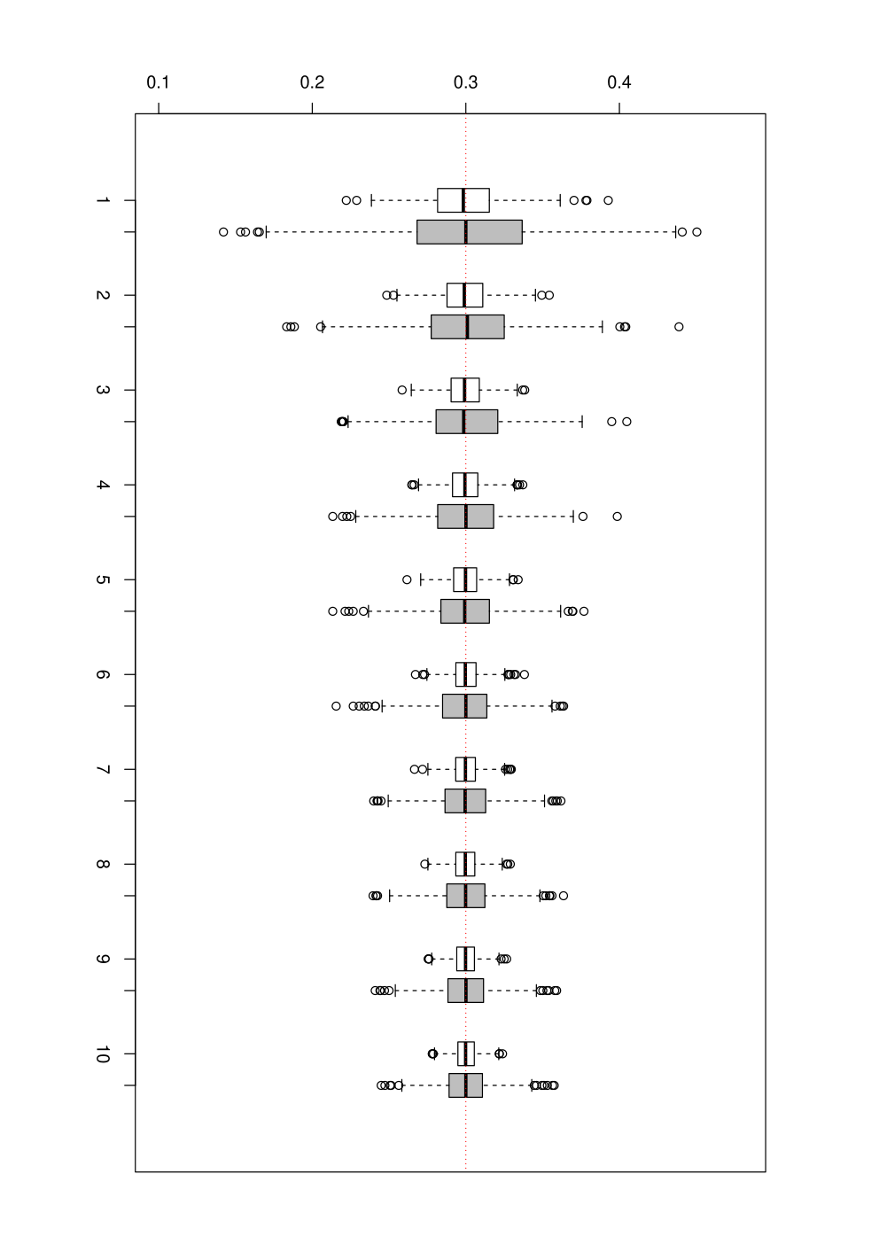
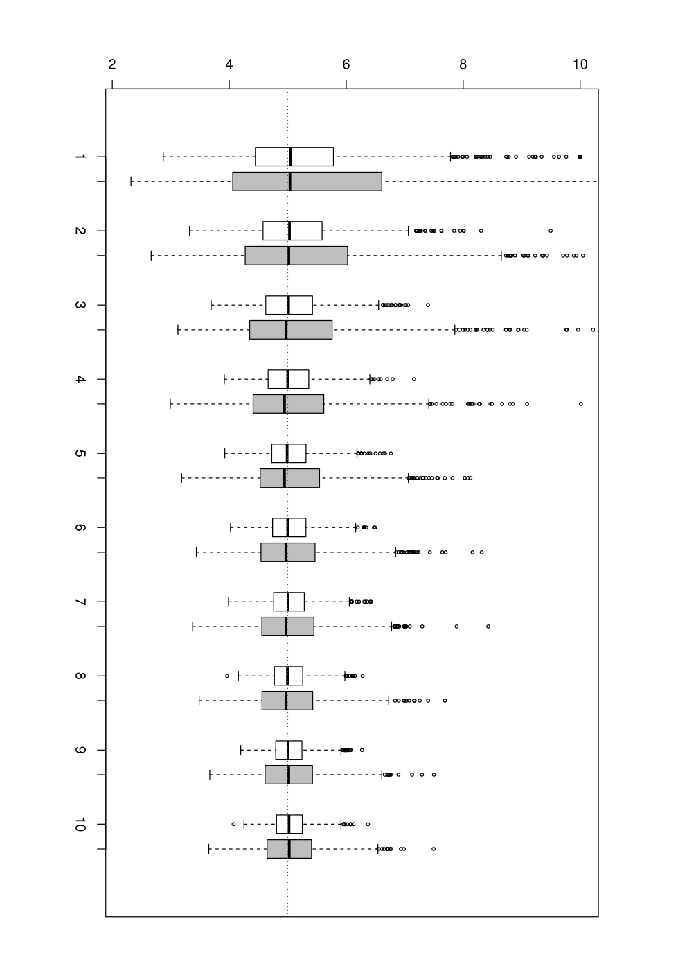
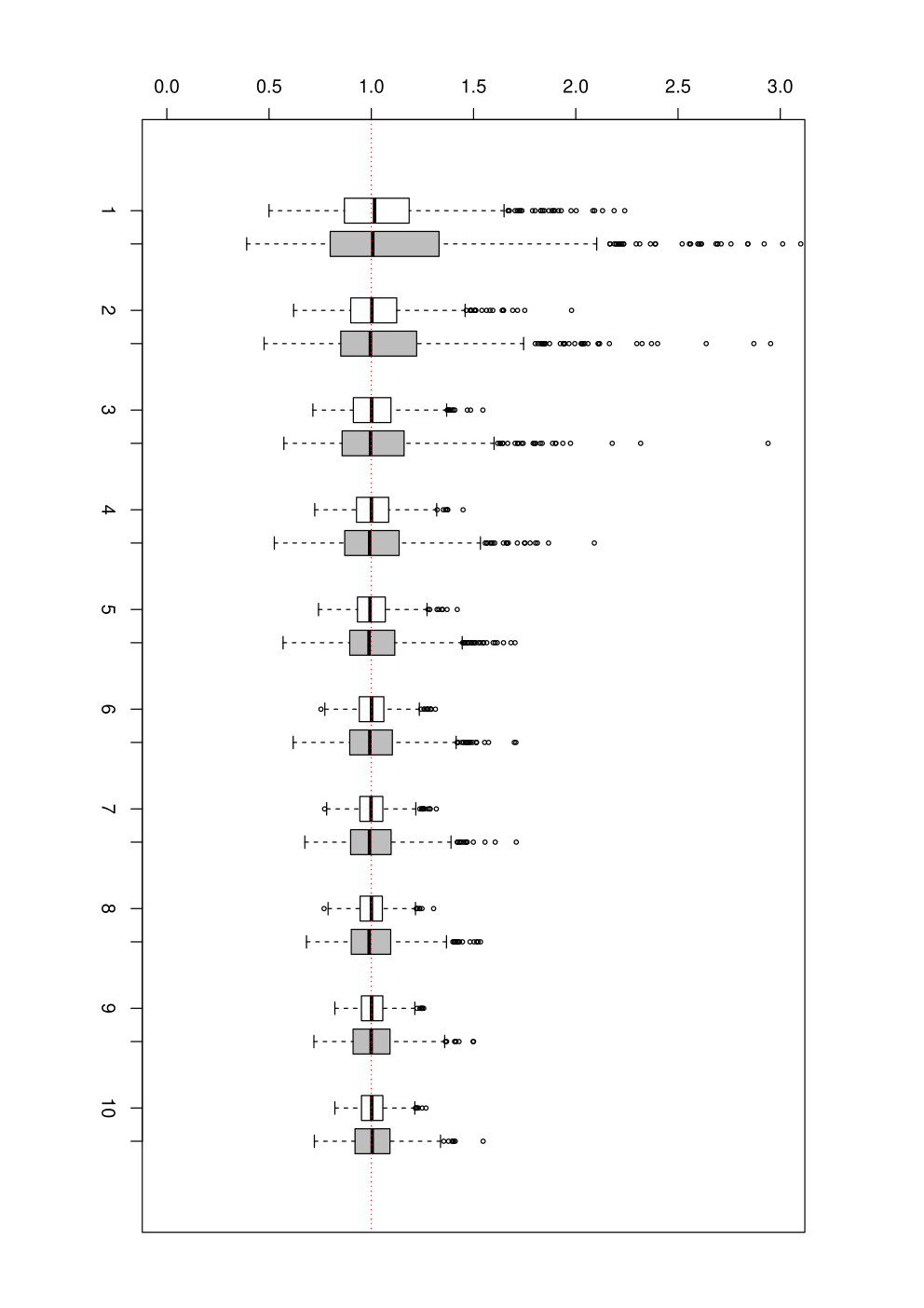
For each of the three simulations, we a priori fix a parameter value ${\theta^{\star}}$ as given in Table 1 and repeat 1 000 times the procedure described below. We first generate a random environment according to $\nu_{\theta^{\star}}$ on the set of sites $\{-10^{4},\dots,10^{4}\}$ . In fact, we do not use the environment values for all the $10^{4}$ negative sites, since only few of these sites are visited by the walk. However the computation cost is very low comparing to the rest of the estimation procedure, and the symmetry is convenient for programming purpose. Then, we run a random walk in this environment and stop it successively at the hitting times $T_{n}$ defined by (2), with $n\in\{10^{3}k;1\leq k\leq 10\}$ . For each stop, we estimate ${\theta^{\star}}$ according to our procedure and Adelman and Enriquez’s one (except for the second simulation). In all three cases, the parameters in Table 1 are chosen such that the RWRE is transient and ballistic to the right. Note that the length of the random walk is not $n$ but rather $T_{n}$ . This quantity varies considerably throughout the three setups and the different iterations. Figure 1 shows (frequency) histograms of the hitting times $T_{n}$ for some selected values $n$ ( $n=$ 1 000, 5 000 and 10 000), obtained from 1 000 iterations of the procedures in each of the three different setups.

Simulation	Fixed parameter	Estimated parameter
Example I	$(a_{1},a_{2})=(0.4,0.7)$	$p^{\star}=0.3$
Example II	-	$(a_{1}^{\star},a_{2}^{\star},p^{\star})=(0.4,0.7,0.3)$
Example III	-	$(\alpha^{\star},\beta^{\star})=(5,1)$

Table 1: Parameter values for each experiment.

Figure 2 shows the boxplots of our estimator and Adelman and Enriquez’s estimator obtained from 1 000 iterations of the procedures in the two Examples I and III, while Figure 3 only displays these boxplots for our estimator in Example II. First, we shall notify that in order to simplify the visualisation of the results, we removed in the boxplots corresponding to Example I (Bottom panel of Figure 2) about 0.8% of outliers values from our estimator, that where equal to 1. Indeed in those cases, the likelihood optimisation procedure did not converge, resulting in the arbitrary value $\hat{p}=1$ . In the same way for Example III, we removed from the figure parameter values of Adelman and Enriquez’s estimator that were too large. It corresponds to about 0.7% of values $\hat{\alpha}$ larger than 10 (for estimating $\alpha^{\star}=5$ ) and about 0.2% of values $\hat{\beta}$ larger than 3 (for estimating $\beta^{\star}=1$ ). In the following discussion, we neglect these rather rare numerical issues. We first observe that the accuracies of the procedures increase with the value of $n$ and thus the walk length $T_{n}$ . We also note that both procedures are unbiased. The main difference comes when considering the variance of each procedure (related to the width of the boxplots): our procedure exhibits a much smaller variance than Adelman and Enriquez’s one as well as a smaller number of outliers. We stress that Adelman and Enriquez’s estimator is expected to exhibit its best performances in Examples I and III that are considered here. Indeed, in these cases, inverting the system of equations that link the parameter to the moments distribution is particularly simple.

Refer to caption — Figure 1: Histograms of the hitting times $T_{n}$ obtained from 1 000 iterations in each of the two setups and for values $n$ equal to 1 000 (white), 5 000 (grey) and 10 000 (hatched). Top panel: Example I; bottom panel: Example III.

References

Adelman and Enriquez (2004) Adelman, O. and N. Enriquez (2004). Random walks in random environment: what a single trajectory tells. Israel J. Math. 142, 205–220.
Alemany et al. (2012) Alemany, A., A. Mossa, I. Junier, and F. Ritort (2012). Experimental free-energy measurements of kinetic molecular states using fluctuation theorems. Nat Phys 8(9), 688–694.
Andreoletti and Diel (2012) Andreoletti, P. and R. Diel (2012). DNA unzipping via stopped birth and death processes with unknown transition probabilities. Applied Mathematics Research eXpress.
Baldazzi et al. (2007) Baldazzi, V., S. Bradde, S. Cocco, E. Marinari, and R. Monasson (2007). Inferring DNA sequences from mechanical unzipping data: the large-bandwidth case. Phys. Rev. E 75, 011904.
Baldazzi et al. (2006) Baldazzi, V., S. Cocco, E. Marinari, and R. Monasson (2006). Inference of DNA sequences from mechanical unzipping: an ideal-case study. Phys. Rev. Lett. 96, 128102.
Bizarro et al. (2012) Bizarro, C. V., A. Alemany, and F. Ritort (2012). Non-specific binding of na+ and mg2+ to RNA determined by force spectroscopy methods. Nucleic Acids Research.
Chernov (1967) Chernov, A. (1967). Replication of a multicomponent chain by the lightning mechanism. Biofizika 12, 297–301.
Cocco and Monasson (2008) Cocco, S. and R. Monasson (2008). Reconstructing a random potential from its random walks. EPL (Europhysics Letters) 81(2), 20002.
Hughes (1996) Hughes, B. D. (1996). Random walks and random environments. Vol. 2. Oxford Science Publications. New York: The Clarendon Press Oxford University Press. Random environments.
Huguet et al. (2009) Huguet, J. M., N. Forns, and F. Ritort (2009, Dec). Statistical properties of metastable intermediates in DNA unzipping. Phys. Rev. Lett. 103, 248106.
Kesten et al. (1975) Kesten, H., M. V. Kozlov, and F. Spitzer (1975). A limit law for random walk in a random environment. Compositio Math. 30, 145–168.
Key (1987) Key, E. S. (1987). Limiting distributions and regeneration times for multitype branching processes with immigration in a random environment. Ann. Probab. 15(1), 344–353.
Koch et al. (2002) Koch, S. J., A. Shundrovsky, B. C. Jantzen, and M. D. Wang (2002). Probing protein-DNA interactions by unzipping a single DNA double helix. Biophysical Journal 83(2), 1098 – 1105.
Norris (1998) Norris, J. R. (1998). Markov chains, Volume 2 of Cambridge Series in Statistical and Probabilistic Mathematics. Cambridge: Cambridge University Press.
Ribezzi-Crivellari et al. (2011) Ribezzi-Crivellari, M., M. Wagner, and F. Ritort (2011). Bayesian approach to the determination of the kinetic parameters of DNA hairpins under tension. Journal of Nonlinear Mathematical Physics 18(supp02), 397–410.
Roitershtein (2007) Roitershtein, A. (2007). A note on multitype branching processes with immigration in a random environment. Ann. Probab. 35(4), 1573–1592.
Shiryaev (1996) Shiryaev, A. N. (1996). Probability (Second ed.), Volume 95 of Graduate Texts in Mathematics. New York: Springer-Verlag.
Solomon (1975) Solomon, F. (1975). Random walks in a random environment. Ann. Probability 3, 1–31.
van der Vaart (1998) van der Vaart, A. W. (1998). Asymptotic statistics, Volume 3 of Cambridge Series in Statistical and Probabilistic Mathematics. Cambridge: Cambridge University Press.
Wald (1949) Wald, A. (1949). Note on the consistency of the maximum likelihood estimate. Ann. Math. Statistics 20, 595–601.
Zeitouni (2004) Zeitouni, O. (2004). Random walks in random environment. In Lectures on probability theory and statistics, Volume 1837 of Lecture Notes in Math., pp. 189–312. Berlin: Springer.