跳到论文正文
W Papers独立论文阅读器 arXiv:1210.6305 论文正文 计算阅读时间 · 0%
引用这篇论文根据当前论文元数据生成,正式投稿前建议核对。


License: arXiv.org perpetual non-exclusive license
arXiv:1210.6305v1 [math.AG] 23 Oct 2012

COMPATIBLY SPLIT SUBVARIETIES OF THE HILBERT SCHEME OF POINTS IN THE PLANE

A Dissertation

Presented to the Faculty of the Graduate School

of Cornell University

in Partial Fulfillment of the Requirements for the Degree of

Doctor of Philosophy

by

Jenna Beth Rajchgot

January 2013

©\copyright 2013 Jenna Beth Rajchgot
ALL RIGHTS RESERVED

COMPATIBLY SPLIT SUBVARIETIES OF THE HILBERT SCHEME OF POINTS IN THE PLANE

Jenna Beth Rajchgot, Ph.D.

Cornell University 2013

Let kk be an algebraically closed field of characteristic p>2p>2. By a result of Kumar and Thomsen (see [KT01]), the standard Frobenius splitting of 𝔸k2\mathbb{A}^{2}_{k} induces a Frobenius splitting of Hilbn​(𝔸k2)\textrm{Hilb}^{n}(\mathbb{A}_{k}^{2}). In this thesis, we investigate the question, “what is the stratification of Hilbn​(𝔸k2)\textrm{Hilb}^{n}(\mathbb{A}_{k}^{2}) by all compatibly Frobenius split subvarieties?”

We provide the answer to this question when n≤4n\leq 4 and give a conjectural answer when n=5n=5. We prove that this conjectural answer is correct up to the possible inclusion of one particular one-dimensional subvariety of Hilb5​(𝔸k2)\textrm{Hilb}^{5}(\mathbb{A}^{2}_{k}), and we show that this particular one-dimensional subvariety is not compatibly split for at least those primes pp satisfying 2<p≤232<p\leq 23.

Next, we restrict the splitting of Hilbn​(𝔸k2)\textrm{Hilb}^{n}(\mathbb{A}_{k}^{2}) (now for arbitrary nn) to the affine open patch U⟨x,yn⟩U_{\langle x,y^{n}\rangle} and describe all compatibly split subvarieties of this patch and their defining ideals. We find degenerations of these subvarieties to Stanley-Reisner schemes, explicitly describe the associated simplicial complexes, and use these complexes to prove that certain compatibly split subvarieties of U⟨x,yn⟩U_{\langle x,y^{n}\rangle} are Cohen-Macaulay.

BIOGRAPHICAL SKETCH

Jenna Rajchgot was raised in Thornhill, Ontario, Canada, a suburb of Toronto. She graduated from Thornhill Secondary School in 2003 and went on to study mathematics at Queen’s University in Kingston, Ontario. She graduated from Queen’s with a B.Sc.H. degree in the spring of 2007. The following August, she entered the math Ph.D. program at Cornell University. She completed her dissertation in August 2012 under the supervision of Professor Allen Knutson.

ACKNOWLEDGEMENTS

This thesis could not have been written without the constant guidance of my advisor, Allen Knutson. Allen helped me every step of the way; he provided the motivating problem, patiently explained relevant background material, and offered numeous helpful suggestions at our frequent meetings. I learned more mathematics from Allen than from any other source and I have a greater appreciation of the subject thanks to him. I feel very fortunate to have worked under Allen’s supervision and I’m pleased to thank him here.

I would also like to thank my other committee members, Tara Holm and Mike Stillman, for helpful discussions, for interesting courses and seminars, and for commenting on previous drafts of this thesis.

I am grateful to David Speyer for graciously allowing an unpublished theorem and proof of his to be included in this thesis. I also wish to thank Allen Knutson, Thomas Lam, and David Speyer for permitting me to include an unpublished version of their algorithm for finding compatibly split subvarieties.

Over my five years at Cornell, I had the pleasure of working with a number of students and postdocs in the mathematics department. I would especially like to acknowledge Mathias Lederer as I had many enjoyable and enlightening conversations with him. In addition, Mathias kindly taught me to use a program that he wrote for computing on open patches of Hilbert schemes of points. This program was very useful when performing computations relevant to this thesis.

On a personal note, I would like to thank my friends, especially Amy, Joeun, Kathryn, Michelle, and Voula, for providing me a great deal of encouragement while I was writing this thesis, and for making my five years in Ithaca very enjoyable.

Finally, I would like to thank my parents Percy and Rochelle, my brother Jason, and my partner Cameron Franc for all of their love and support.

I was supported by the Cornell mathematics department and by the Natural Sciences and Engineering Research Council of Canada (NSERC).

TABLE OF CONTENTS

INTRODUCTION

Let kk be an algebraically closed field of characteristic p>2p>2, and let XX be a quasiprojective smooth surface defined over kk. The Hilbert scheme of nn points on XX, denoted Hilbn​(X)\textrm{Hilb}^{n}(X), is the 2​n2n-dimensional smooth scheme (see [Fog68]) which parametrizes all dimension-00, degree-nn subschemes of XX. If XX is Frobenius split, then Hilbn​(X)\textrm{Hilb}^{n}(X) is Frobenius split (see [KT01]). More specifically, if XX is Frobenius split compatibly with the anticanonical divisor DD, then Hilbn​(X)\textrm{Hilb}^{n}(X) is Frobenius split compatibly with the anticanonical divisor described set-theoretically by

{q∈Hilbn​(X)|Supp​(q)∩D≠∅}.\{q\in\textrm{Hilb}^{n}(X)~|~\textrm{Supp}(q)\cap D\neq\emptyset\}.

In this thesis, we are interested in the case X=𝔸k2X=\mathbb{A}_{k}^{2} and D={xy=0}D=\{xy=0\}. Our motivating problem is to understand the stratification of Hilbn​(𝔸k2)\textrm{Hilb}^{n}(\mathbb{A}_{k}^{2}) by all of its finitely many (see [KM09], [Sch09]) compatibly split subvarieties (with respect to this particular splitting).

Refer to caption
Figure 1: The compatibly split subvarieties of Hilb2​(𝔸k2)\textrm{Hilb}^{2}(\mathbb{A}^{2}_{k})

To gain some intuition, we consider the n=2n=2 case. The stratification of Hilb2​(𝔸k2)\textrm{Hilb}^{2}(\mathbb{A}^{2}_{k}) by all compatibly split subvarieties is shown in Figure 1. We have drawn a “stratum representative” (see Subsection 2.1.2) to correspond to an entire compatibly split subvariety. For example, the picture where the two points are at the origin and on a diagonal line represents the punctual Hilbert scheme, denoted Hilb02​(𝔸k2)\textrm{Hilb}^{2}_{0}(\mathbb{A}^{2}_{k}), which parametrizes dimension-00, length-22 subschemes of 𝔸k2\mathbb{A}^{2}_{k} that are supported at the origin. Note that Hilb02​(𝔸k2)≅ℙk1\textrm{Hilb}^{2}_{0}(\mathbb{A}^{2}_{k})\cong\mathbb{P}^{1}_{k}.

To gain further intuition into our problem, we remark (see Proposition 2.1.1) that finding all compatibly split subvarieties of Hilbn​(𝔸k2)\textrm{Hilb}^{n}(\mathbb{A}_{k}^{2}) is equivalent to finding all compatibly split subvarieties Z⊆Hilbm​(𝔸k2)Z\subseteq\textrm{Hilb}^{m}(\mathbb{A}^{2}_{k}) for m≤nm\leq n, where ZZ is a subvariety the punctual Hilbert scheme Hilb0m​(𝔸k2)\textrm{Hilb}^{m}_{0}(\mathbb{A}^{2}_{k}). More precisely, for sufficiently large primes pp, Y⊆Hilbn​(𝔸k2)Y\subseteq\textrm{Hilb}^{n}(\mathbb{A}_{k}^{2}) is a compatibly split subvariety if and only if YY is the closure in Hilbn​(𝔸k2)\textrm{Hilb}^{n}(\mathbb{A}_{k}^{2}) of the (set-theoretic) image of a map

i:Hilbr(“punctured y-axis”)×Hilbs(“punctured x-axis”)×Hilbt(𝔸k2∖{xy=0})×Zi:\textrm{Hilb}^{r}(\textrm{``punctured y-axis''})\times\textrm{Hilb}^{s}(\textrm{``punctured x-axis''})\times\textrm{Hilb}^{t}(\mathbb{A}^{2}_{k}\setminus\{xy=0\})\times Z
→Hilbn​(𝔸k2)\rightarrow\textrm{Hilb}^{n}(\mathbb{A}_{k}^{2})
(I1,I2,I3,I4)↦I1∩I2∩I3∩I4(I_{1},I_{2},I_{3},I_{4})\mapsto I_{1}\cap I_{2}\cap I_{3}\cap I_{4}

for some r,s,t≥0r,s,t\geq 0 with r+s+t≤nr+s+t\leq n and for some compatibly split Z⊆Hilbn−r−s−t​(𝔸k2)Z\subseteq\textrm{Hilb}^{n-r-s-t}(\mathbb{A}^{2}_{k}) with the property that Z⊆Hilb0n−r−s−t​(𝔸k2)Z\subseteq\textrm{Hilb}^{n-r-s-t}_{0}(\mathbb{A}^{2}_{k}). Of course, in order to understand all compatibly split subvarieties of Hilbn​(𝔸k2)\textrm{Hilb}^{n}(\mathbb{A}_{k}^{2}), we must still compute all of these Z⊆Hilb0m​(𝔸k2)Z\subseteq\textrm{Hilb}_{0}^{m}(\mathbb{A}^{2}_{k}), m≤nm\leq n.

One method for finding all compatibly split subvarieties for small nn is to utilize an algorithm of Allen Knutson, Thomas Lam, and David Speyer. We explain this algorithm in the Frobenius splitting background section and use it in Subsection 2.2.1 to produce the stratification of Hilb2​(𝔸k2)\textrm{Hilb}^{2}(\mathbb{A}^{2}_{k}) pictured above. In Subsection 2.2.2, we use other tools (primarily the moment polyhedron of Hilbn​(𝔸k2)\textrm{Hilb}^{n}(\mathbb{A}_{k}^{2})) to produce all compatibly split subvarieties of Hilbn​(𝔸k2)\textrm{Hilb}^{n}(\mathbb{A}_{k}^{2}) for n≤4n\leq 4, as well as provide a conjectural list of all compatibly split subvarieties of Hilb5​(𝔸k2)\textrm{Hilb}^{5}(\mathbb{A}^{2}_{k}). We prove that this conjectural list is correct up to the possible inclusion of one particular one-dimensional subvariety of Hilb5​(𝔸k2)\textrm{Hilb}^{5}(\mathbb{A}^{2}_{k}), and we show that this particular one-dimensional subvariety is not compatibly split for at least those primes pp satisfying 2<p≤232<p\leq 23.

After the discussion of the n=5n=5 case, we restict our attention to the open affine patch

U⟨x,yn⟩={I∈Hilbn​(𝔸k2)|{1,y,…,yn−1}​ is a ​k​-vector space basis of ​k​[x,y]/I}.U_{\langle x,y^{n}\rangle}=\{I\in\textrm{Hilb}^{n}(\mathbb{A}_{k}^{2})~|~\{1,y,\dots,y^{n-1}\}\textrm{ is a }k\textrm{-vector space basis of }k[x,y]/I\}.

This patch has an induced Frobenius splitting and so we may ask the question, “what are all of the compatibly split subvarieties of U⟨x,yn⟩U_{\langle x,y^{n}\rangle} with the induced splitting?” In Section 2.3, we answer this question for general nn. We describe the defining ideals of these subvarieties and we find degenerations to Stanley-Reisner schemes. We provide an explicit description of the simplicial complexes associated to these Stanley-Reisner schemes and use these complexes to prove that certain compatibly split subvarieties of U⟨x,yn⟩U_{\langle x,y^{n}\rangle} are Cohen-Macaulay.

This thesis has two chapters. Chapter 1 discusses relevant background material, an unpublished result of David E Speyer, and the unpublished Knutson-Lam-Speyer algorithm for finding compatibly split subvarieties. Chapter 2 addresses the material described above.

Macaulay 2 [GS] was used to perform numerous computations leading to the results appearing in Chapter 2 of this thesis. Sage [S+] (with the FLINT library) was used to perform some of the computations appearing in the discussion of the compatibly split subvarieties of Hilb5​(𝔸k2)\textrm{Hilb}^{5}(\mathbb{A}^{2}_{k}).

Chapter 1 Background

1.1 The Hilbert scheme of points in the plane

1.1.1 Basic notions

Material in this subsection is taken primarily from [Nak99, Chapter 1].

Let kk be an algebraically closed field. The Hilbert scheme of 𝐧\mathbf{n} points in the affine plane, Hilbn​(𝔸k2)\textrm{Hilb}^{n}(\mathbb{A}_{k}^{2}), is the scheme parametrizing all zero-dimensional, length-nn subschemes of 𝔸k2\mathbb{A}^{2}_{k}. More precisely, Hilbn​(𝔸k2)\textrm{Hilb}^{n}(\mathbb{A}_{k}^{2}) represents the contravariant functor

ℋ​i​l​b𝔸k2n:Schemes→Sets\mathcal{H}ilb^{n}_{\mathbb{A}_{k}^{2}}:\textrm{Schemes}\rightarrow\textrm{Sets}

ℋilb𝔸k2n(U)={Z⊆U×𝔸k2Z​is a closed subscheme andπ:Z→U​is flat with dimension-​0​,​length-​n​fibers}.\mathcal{H}ilb^{n}_{\mathbb{A}_{k}^{2}}(U)=\left\{Z\subseteq U\times\mathbb{A}_{k}^{2}~\begin{array}[]{|c}$Z$~\textrm{is a closed subscheme and}\\ \pi:Z\rightarrow U~\textrm{is flat with dimension-}0\textrm{,}~\textrm{length-}n~\textrm{fibers}\\ \end{array}\right\}.
Example 1.1.1.
  1. 1.

    The Hilbert scheme of 11 point in the plane is isomorphic to 𝔸k2\mathbb{A}^{2}_{k}.

  2. 2.

    A zero-dimensional, length-22 subscheme of 𝔸k2\mathbb{A}^{2}_{k} is determined by either (i) two distinct unordered locations (x1,y1),(x2,y2)∈𝔸k2(x_{1},y_{1}),(x_{2},y_{2})\in\mathbb{A}^{2}_{k}, or (ii) one location (x,y)∈𝔸k2(x,y)\in\mathbb{A}^{2}_{k} along with a projective vector v∈ℙk1v\in\mathbb{P}^{1}_{k}. Indeed, Hilb2​(𝔸k2)≅B​lΔ​(𝔸k2×𝔸k2)/S2\textrm{Hilb}^{2}(\mathbb{A}^{2}_{k})\cong Bl_{\Delta}({\mathbb{A}^{2}_{k}\times\mathbb{A}^{2}_{k}})/S_{2} where B​lΔ​(𝔸k2×𝔸k2)Bl_{\Delta}({\mathbb{A}^{2}_{k}\times\mathbb{A}^{2}_{k}}) denotes the blow-up of 𝔸k2×𝔸k2\mathbb{A}^{2}_{k}\times\mathbb{A}^{2}_{k} along the diagonal locus Δ:={((x,y),(x,y))|(x,y)∈𝔸k2}\Delta:=\{((x,y),(x,y))~|~(x,y)\in\mathbb{A}^{2}_{k}\}.

Consider the action of the symmetric group SnS_{n} on (𝔸k2)n(\mathbb{A}^{2}_{k})^{n} by permuting the various copies of 𝔸2\mathbb{A}^{2}. Taking the quotient of (𝔸k2)n(\mathbb{A}^{2}_{k})^{n} by SnS_{n} yields the Chow variety, the scheme of nn unlabelled locations in the plane. This scheme is often denoted by Sn​(𝔸k2)S^{n}(\mathbb{A}^{2}_{k}). An element of Sn​(𝔸k2)S^{n}(\mathbb{A}^{2}_{k}) is written as a sum

∑(x,y)∈𝔸k2a(x,y)​[(x,y)]\sum_{(x,y)\in\mathbb{A}^{2}_{k}}a_{(x,y)}[(x,y)]

where the coefficients {a(x,y)|(x,y)∈𝔸k2}\{a_{(x,y)}~|~(x,y)\in\mathbb{A}^{2}_{k}\} are non-negative integers that sum to nn.

Definition 1.1.2.

The Hilbert-Chow morphism

Ψ:Hilbn​(𝔸k2)→Sn​(𝔸k2)\Psi:\textrm{Hilb}^{n}(\mathbb{A}_{k}^{2})\rightarrow S^{n}(\mathbb{A}_{k}^{2})

is the map which takes each zero-dimensional, length-nn subscheme of 𝔸k2\mathbb{A}^{2}_{k} to its support with multiplicities. That is,

Ψ:Z↦∑x∈𝔸k2length​(Zx)​[x].\Psi:Z\mapsto\sum_{x\in\mathbb{A}^{2}_{k}}\textrm{length}(Z_{x})[x].

Notice that SnS_{n} acts freely on the open set V⊆(𝔸k2)nV\subseteq(\mathbb{A}^{2}_{k})^{n} where all of the nn locations are distinct. Thus, the Chow variety is smooth along V/SnV/S_{n}. Sn​(𝔸k2)S^{n}(\mathbb{A}^{2}_{k}) is singular along the closed subvariety where at least two points collide.

Theorem 1.1.3.

[Fog68]

  1. 1.

    Ψ:Hilbn​(𝔸k2)→(𝔸k2)n/Sn\Psi:\textrm{Hilb}^{n}(\mathbb{A}_{k}^{2})\rightarrow(\mathbb{A}_{k}^{2})^{n}/S_{n} defined in Definition 1.1.2 is a birational, projective morphism of schemes. It is an isomorphism over the open set where all points are distinct.

  2. 2.

    Hilbn​(𝔸k2)\textrm{Hilb}^{n}(\mathbb{A}_{k}^{2}) is connected and smooth. Thus, the Hilbert-Chow morphism is a resolution of singularities.

As a corollary, Hilbn​(𝔸k2)\textrm{Hilb}^{n}(\mathbb{A}_{k}^{2}) is irreducible. In addition, because the Chow variety is 2​n2n-dimensional and the Hilbert-Chow morphism is birational, Hilbn​(𝔸k2)\textrm{Hilb}^{n}(\mathbb{A}_{k}^{2}) is also 2​n2n-dimensional.

1.1.2 An open cover

In this subsection, we describe an open cover of Hilbn​(𝔸k2)\textrm{Hilb}^{n}(\mathbb{A}_{k}^{2}) indexed by the colength-nn monomial ideals. Our main references for this material are [Hai98], [MS05, Chapter 18], and [Led11].

Definition 1.1.4.

Let λ\lambda be a colength-nn monomial ideal. Define Uλ⊆Hilbn​(𝔸k2)U_{\lambda}\subseteq\textrm{Hilb}^{n}(\mathbb{A}_{k}^{2}) to be the set of ideals II such that the monomials outside of λ\lambda form a kk-vector space basis for k⁡[x,y]/Ik[x,y]/I.

Notice that the set of all UλU_{\lambda} cover Hilbn​(𝔸k2)\textrm{Hilb}^{n}(\mathbb{A}_{k}^{2}). Indeed, if I∈Hilbn​(𝔸k2)I\in\textrm{Hilb}^{n}(\mathbb{A}_{k}^{2}) and >> is a term order, the initial ideal init>​(I)\textrm{init}_{>}(I) (see Subsection 1.4.1 for relevant definitions) is a colength-nn monomial ideal and the nn monomials outside of init>​(I)\textrm{init}_{>}(I) form a kk-vector space basis for k⁡[x,y]/Ik[x,y]/I. Thus, I∈Uinit>​(I)I\in U_{\textrm{init}_{>}(I)}.

Any ideal I∈UλI\in U_{\lambda} has a unique set of generators of the form

{xrys−∑xh​yl∉λch,lr,sxhyl|xrys∈λ,ch,lr,s∈k}.\left\{x^{r}y^{s}-\sum_{x^{h}y^{l}\notin\lambda}c^{r,s}_{h,l}x^{h}y^{l}~|~x^{r}y^{s}\in\lambda,c^{r,s}_{h,l}\in k\right\}.

Thus, the ch,lr,sc^{r,s}_{h,l} are coordinates on UλU_{\lambda}. Furthermore, if g∈Ig\in I, then x⋅g∈Ix\cdot g\in I and y⋅g∈Iy\cdot g\in I. These conditions yield relations in the various ch,lr,sc^{r,s}_{h,l}. To be precise, suppose that g=xr​ys−∑xh​yl∉λch,lr,s​xh​ylg=x^{r}y^{s}-\sum_{x^{h}y^{l}\notin\lambda}c^{r,s}_{h,l}x^{h}y^{l} is an element of II. Then,

x⋅g=xr+1​ys−∑xh​yl∉λch,lr,s​xh+1​yl​(∗)x\cdot g=x^{r+1}y^{s}-\sum_{x^{h}y^{l}\notin\lambda}c^{r,s}_{h,l}x^{h+1}y^{l}~~~(*)

is also in II. Notice that some of the xh+1​ylx^{h+1}y^{l} appearing in (∗)(*) are in λ\lambda. We can therefore replace these xh+1​yl∈λx^{h+1}y^{l}\in\lambda using xh+1​yl−∑xh′​yl′ch′,l′h+1,l​xh′​yl′∈Ix^{h+1}y^{l}-\sum_{x^{h^{\prime}}y^{l^{\prime}}}c^{h+1,l}_{h^{\prime},l^{\prime}}x^{h^{\prime}}y^{l^{\prime}}\in I to see that

xr+1ys−(∑xh+1​yl∉λch,lr,sxh+1yl+∑xh+1​yl∈λch,lr,s∑xh′​yl′ch′,l′h+1,lxh′yl′)(∗∗)x^{r+1}y^{s}-\left(\sum_{x^{h+1}y^{l}\notin\lambda}c^{r,s}_{h,l}x^{h+1}y^{l}+\sum_{x^{h+1}y^{l}\in\lambda}c^{r,s}_{h,l}\sum_{x^{h^{\prime}}y^{l^{\prime}}}c^{h+1,l}_{h^{\prime},l^{\prime}}x^{h^{\prime}}y^{l^{\prime}}\right)~~~(**)

is an element of II. On the other hand,

xr+1ys−∑xh​yl∉λch,lr+1,sxhyl(∗∗∗)x^{r+1}y^{s}-\sum_{x^{h}y^{l}\notin\lambda}c^{r+1,s}_{h,l}x^{h}y^{l}~~~(***)

is also in II. Equating coefficients in (∗∗)(**) with those in (∗∗∗)(***) yield relations amongst various ch,lr,sc^{r,s}_{h,l}. Let JλJ_{\lambda} denote the ideal generated by these relations, along with the relations obtained by interchanging the roles of xx and yy in the above computation.

Proposition 1.1.5.

The sets UλU_{\lambda} are open affine subvarieties that cover Hilbn​(𝔸k2)\textrm{Hilb}^{n}(\mathbb{A}_{k}^{2}). The affine coordinate ring is given by k[{ch,lr,s|xrys∈λ,xhyl∉λ}]/Jλk[\{c^{r,s}_{h,l}~|~x^{r}y^{s}\in\lambda,~x^{h}y^{l}\notin\lambda\}]/J_{\lambda}.

Example 1.1.6.

Let λ=⟨x,yn⟩\lambda=\langle x,y^{n}\rangle. Then U⟨x,yn⟩U_{\langle x,y^{n}\rangle} consists of all I∈Hilbn​(𝔸k2)I\in\textrm{Hilb}^{n}(\mathbb{A}_{k}^{2}) such that {1,y,…,yn−1}\{1,y,\dots,y^{n-1}\} is a kk-vector space basis for k⁡[x,y]/Ik[x,y]/I. In addition, each I∈U⟨x,yn⟩I\in U_{\langle x,y^{n}\rangle} is generated by the set of polynomials

{xr​ys−c0,n−1r,s​yn−1−⋯−c0,1r,s​y−c0,0r,s|xr​ys∈⟨x,yn⟩}.\{x^{r}y^{s}-c^{r,s}_{0,n-1}y^{n-1}-\cdots-c^{r,s}_{0,1}y-c^{r,s}_{0,0}~|~x^{r}y^{s}\in\langle x,y^{n}\rangle\}.

Notice that not all of these generators are necessary. In fact, each I∈U⟨x,yn⟩I\in U_{\langle x,y^{n}\rangle} is minimally generated by a set of the form

G={yn−c0,n−10,n​yn−1−⋯−c0,10,n​y−c0,00,n,x−c0,n−11,0​yn−1−⋯−c0,11,0​y−c0,01,0}.G=\{y^{n}-c^{0,n}_{0,n-1}y^{n-1}-\cdots-c^{0,n}_{0,1}y-c^{0,n}_{0,0},~x-c^{1,0}_{0,n-1}y^{n-1}-\cdots-c^{1,0}_{0,1}y-c^{1,0}_{0,0}\}.

Indeed, with respect to the Lex term order with x≫yx\gg y, GG is a Gröbner basis with initial ideal ⟨x,yn⟩\langle x,y^{n}\rangle. Thus, I∈U⟨x,yn⟩I\in U_{\langle x,y^{n}\rangle} if and only if init​(I)=⟨x,yn⟩\textrm{init}(I)=\langle x,y^{n}\rangle.

The number of generators of the coordinate ring of UλU_{\lambda} can be reduced significantly from that in Proposition 1.1.5.

Definition 1.1.7.

Let λ\lambda be a colength-nn monomial ideal. The standard set of λ\mathbf{\lambda}, which we denote by SλS_{\lambda}, is the set of all (i,j)∈ℕ2(i,j)\in\mathbb{N}^{2} such that xi​yjx^{i}y^{j} is a monomial outside of λ\lambda. The border of λ\mathbf{\lambda}, which we denote by BλB_{\lambda}, is the set of all (i,j)∈ℕ2∖Sλ(i,j)\in\mathbb{N}^{2}\setminus S_{\lambda} such that (i−1,j)∈Sλ(i-1,j)\in S_{\lambda} or (i,j−1)∈Sλ(i,j-1)\in S_{\lambda}.

Example 1.1.8.

Let λ=⟨x2,x​y2,y3⟩∈Hilb5​(𝔸k2)\lambda=\langle x^{2},xy^{2},y^{3}\rangle\in\textrm{Hilb}^{5}(\mathbb{A}^{2}_{k}). The monomials outside of λ\lambda are {1,x,y,x​y,y2}\{1,x,y,xy,y^{2}\}. Therefore, Sλ={(0,0),(1,0),(0,1),(1,1),(0,2)}S_{\lambda}=\{(0,0),(1,0),(0,1),(1,1),(0,2)\} and Bλ={(2,0),(2,1),(1,2),(0,3)}B_{\lambda}=\{(2,0),(2,1),(1,2),(0,3)\}.

Often, we draw the Young diagram (using French notation) associated to the monomial ideal λ\lambda instead of writing down the standard set. Notice that the Young diagram and the standard set give equivalent information.

Theorem 1.1.9.

Let λ\lambda be a colength-nn monomial ideal. Let SλS_{\lambda} denote its standard set and let BλB_{\lambda} denote its border. The coordinate ring of UλU_{\lambda} is generated by those ch​lr​sc^{rs}_{hl} such that (r,s)∈Bλ(r,s)\in B_{\lambda} and (h,l)∈Sλ(h,l)\in S_{\lambda}.

Before concluding this subsection, we note that for many colength-nn monomial ideals λ\lambda, UλU_{\lambda} is isomorphic to 𝔸k2​n\mathbb{A}^{2n}_{k}. For example, when n≤4n\leq 4, UλU_{\lambda} is always isomorphic to 𝔸k2​n\mathbb{A}^{2n}_{k}.

1.1.3 A torus action

The torus T2=𝔾m2T^{2}=\mathbb{G}_{m}^{2} acts algebraically on 𝔸k2\mathbb{A}^{2}_{k} by (t1,t2)⋅(x,y)=(t1​x,t2​y)(t_{1},t_{2})\cdot(x,y)=(t_{1}x,t_{2}y). This induces an action on Hilbn​(𝔸k2)\textrm{Hilb}^{n}(\mathbb{A}_{k}^{2}). That is, if I∈Hilbn​(𝔸k2)I\in\textrm{Hilb}^{n}(\mathbb{A}_{k}^{2}), then

(t1,t2)⋅I=⟨f(t1−1x,t2−1y)|f(x,y)∈I⟩.(t_{1},t_{2})\cdot I=\langle f(t_{1}^{-1}x,t_{2}^{-1}y)~|~f(x,y)\in I\rangle.

Notice that the T2T^{2}-fixed points of Hilbn​(𝔸k2)\textrm{Hilb}^{n}(\mathbb{A}_{k}^{2}) are the colength-nn monomial ideals.

Lemma 1.1.10.

Each UλU_{\lambda} is invariant under the T2T^{2}-action. As an element of the coordinate ring, ch,lr,sc^{r,s}_{h,l} has T2T^{2}-weight (h−r,l−s)(h-r,l-s).

Proof.

Suppose I∈UλI\in U_{\lambda} and xr​ys−∑xh​yl∉λch,lr,s​xh​ylx^{r}y^{s}-\sum_{x^{h}y^{l}\notin\lambda}c^{r,s}_{h,l}x^{h}y^{l} is a generator of II. Then,

(t1,t2)⋅(xr​ys−∑xh​yl∉λch,lr,s​xh​yl)=t1−r​t2−s​xr​ys−∑xh​yl∉λch,lr,s​t1−h​t2−l​xh​yl=t1−r​t2−s​(xr​ys−∑xh​yl∉λt1r−h​t2s−l​ch,lr,s​xh​yl)\begin{array}[]{ccc}(t_{1},t_{2})\cdot(x^{r}y^{s}-\sum_{x^{h}y^{l}\notin\lambda}c^{r,s}_{h,l}x^{h}y^{l})&=&t_{1}^{-r}t_{2}^{-s}x^{r}y^{s}-\sum_{x^{h}y^{l}\notin\lambda}c^{r,s}_{h,l}t_{1}^{-h}t_{2}^{-l}x^{h}y^{l}\\ &=&t_{1}^{-r}t_{2}^{-s}(x^{r}y^{s}-\sum_{x^{h}y^{l}\notin\lambda}t_{1}^{r-h}t_{2}^{s-l}c^{r,s}_{h,l}x^{h}y^{l})\end{array}

So, as an element of the coordinate ring of UλU_{\lambda}, ch,lr,sc^{r,s}_{h,l} has weight (h−r,l−s)(h-r,l-s).

Uλ=Spec⁡(k⁡[{ch,lr,s}]/Jλ)U_{\lambda}=\Spec(k[\{c^{r,s}_{h,l}\}]/J_{\lambda}) is T2T^{2}-invariant because JλJ_{\lambda} is T2T^{2}-homogeneous by construction. ∎

We can use the torus action to prove that Hilbn​(𝔸k2)\textrm{Hilb}^{n}(\mathbb{A}_{k}^{2}) is non-singular. To begin, notice that every ideal I∈Hilbn​(𝔸k2)I\in\textrm{Hilb}^{n}(\mathbb{A}_{k}^{2}) has a T2T^{2}-fixed point in the closure of its orbit. (Indeed, with respect to any monomial order, init​(I)∈T2⋅I¯\textrm{init}(I)\in\overline{T^{2}\cdot I}. As init​(I)\textrm{init}(I) is a colength-nn monomial ideal, it is a T2T^{2}-fixed point.) Therefore, if the Hilbert scheme is singular anywhere, it must also be singular at one of the T2T^{2}-fixed points. We will now show that Hilbn​(𝔸k2)\textrm{Hilb}^{n}(\mathbb{A}_{k}^{2}) is non-singular at each T2T^{2}-fixed point.

Definition 1.1.11.

Let λ\lambda be a colength-nn monomial ideal and let SλS_{\lambda} denote its standard set. For each x∈Sλx\in S_{\lambda}, we define the arm, a⁡(x)a(x), and leg, l⁡(x)l(x), as follows: For x=(i,j)∈Sλx=(i,j)\in S_{\lambda},

a⁡(x):={#⁡(i,r)∈Sλ|r>j},l⁡(x):={#⁡(r,j)∈Sλ|r>i}.a(x):=\{\#(i,r)\in S_{\lambda}~|~r>j\},~~~~~l(x):=\{\#(r,j)\in S_{\lambda}~|~r>i\}.
Proposition 1.1.12.

Let λ\lambda be a T2T^{2}-fixed point of Hilbn​(𝔸k2)\textrm{Hilb}^{n}(\mathbb{A}_{k}^{2}). The tangent space Tλ​Hilbn​(𝔸k2)T_{\lambda}\textrm{Hilb}^{n}(\mathbb{A}_{k}^{2}) is a 2​n2n-dimensional T2T^{2}-representation with T2T^{2}-weights

{(−l⁡(x),a⁡(x)+1)|x∈Sλ}∪{(l⁡(x)+1,−a⁡(x))|x∈Sλ}.\{(-l(x),a(x)+1)~|~x\in S_{\lambda}\}\cup\{(l(x)+1,-a(x))~|~x\in S_{\lambda}\}.

We sketch Haiman’s proof (see [Hai98]) of this result.

Proof (sketch).

We show that the Zariski cotangent space 𝔪λ/𝔪λ2\mathfrak{m}_{\lambda}/\mathfrak{m}_{\lambda}^{2} has dimension at most 2​n2n using the following procedure.

  1. 1.

    Work in the open patch UλU_{\lambda} and note that 𝔪λ\mathfrak{m}_{\lambda} is generated by all of the ch,lr,sc^{r,s}_{h,l} in the coordinate ring of UλU_{\lambda}.

  2. 2.

    Let SλS_{\lambda} denote the standard set of λ\lambda. Identify each ch,lr,sc^{r,s}_{h,l} with the vector from (r,s)(r,s) to (h,l)(h,l). Notice that the position of the tail of this vector is an element of ℕ2∖Sλ\mathbb{N}^{2}\setminus S_{\lambda} and that the position of the head of this vector is an element of SλS_{\lambda}.

  3. 3.

    Say that one arrow can be translated to another if there exists a sequence of horizontal and vertical shifts moving the first arrow to the second such that the position of the tail always remains an element of ℕ2∖Sλ\mathbb{N}^{2}\setminus S_{\lambda} and the position of the head is always of the form (a−c,b−d)(a-c,b-d) where (a,b)∈Sλ(a,b)\in S_{\lambda} and (c,d)∈ℤ≥02(c,d)\in\mathbb{Z}_{\geq 0}^{2}. (That is, it is permissible for the head of the arrow to lie below the xx-axis or to the left of the yy-axis.) Show that ch1,l1r1,s1≡ch2,l2r2,s2​(mod ​𝔪λ2)c^{r_{1},s_{1}}_{h_{1},l_{1}}\equiv c^{r_{2},s_{2}}_{h_{2},l_{2}}~(\textrm{mod }\mathfrak{m}_{\lambda}^{2}) if the arrow associated to ch1,l1r1,s1c^{r_{1},s_{1}}_{h_{1},l_{1}} can be translated to the arrow associated to ch2,l2r2,s2c^{r_{2},s_{2}}_{h_{2},l_{2}}. Show that ch,kr,s≡0​(mod ​𝔪λ2)c^{r,s}_{h,k}\equiv 0~(\textrm{mod }\mathfrak{m}_{\lambda}^{2}) if ch,kr,sc^{r,s}_{h,k} can be translated such that the head of the arrow lies below the xx-axis or to the left of the yy-axis.

  4. 4.

    Notice that every arrow can be translated such that one of the following occurs: (i) the head crosses an axis, or (ii) there is an x=(i,j)∈Sλx=(i,j)\in S_{\lambda} such that the head of the arrow is at (i+l⁡(x),j)(i+l(x),j) and the tail is at (i,j+a⁡(x)+1)(i,j+a(x)+1), or (iii) there is an x=(i,j)∈Sλx=(i,j)\in S_{\lambda} such that the head of the arrow is at (i,j+a⁡(x))(i,j+a(x)) and the tail is at (i+l⁡(x)+1,j)(i+l(x)+1,j).

This procedure yields 2​n2n (i.e. 22 for each x∈Sλx\in S_{\lambda}) elements which span 𝔪λ/𝔪λ2\mathfrak{m}_{\lambda}/\mathfrak{m}_{\lambda}^{2}. Thus, the cotangent space is at most 2​n2n-dimensional. Because each T2T^{2}-fixed point lies in the closure of the smooth, 2​n2n-dimensional locus where all points are distinct, the tangent space at each T2T^{2}-fixed point is also at least 2​n2n-dimensional. Furthermore, we can see from the generators constructed above that the Zariski cotangent space has T2T^{2}-weights

{−(−l⁡(x),a⁡(x)+1)|x∈Sλ}∪{−(l⁡(x)+1,−a⁡(x))|x∈Sλ}.\{-(-l(x),a(x)+1)~|~x\in S_{\lambda}\}\cup\{-(l(x)+1,-a(x))~|~x\in S_{\lambda}\}.

∎

Therefore, Hilbn​(𝔸k2)\textrm{Hilb}^{n}(\mathbb{A}_{k}^{2}) is non-singular at each of the T2T^{2}-fixed points. It follows that Hilbn​(𝔸k2)\textrm{Hilb}^{n}(\mathbb{A}_{k}^{2}) is non-singular everywhere.

1.2 Frobenius splitting

In this section, our main source is the textbook [BK05]. As in the text, we let kk be an algebraically closed field of characteristic p>0p>0 and let (X,𝒪X)(X,\mathcal{O}_{X}) be a separated scheme of finite type over kk.

1.2.1 Basic notions

Recall that the absolute Frobenius morphism, F:X→XF:X\rightarrow X, is defined to be the identity map on points and the pt​hp^{th} power map on functions. Then, F♯:𝒪X→F∗​𝒪XF^{\sharp}:\mathcal{O}_{X}\rightarrow F_{*}\mathcal{O}_{X} is an 𝒪X\mathcal{O}_{X}-linear map where the module structure on F∗​𝒪XF_{*}\mathcal{O}_{X} is given by a⋅b=ap​ba\cdot b=a^{p}b for any local sections a,b of 𝒪X\mathcal{O}_{X}.

Definition 1.2.1.

A scheme (X,𝒪X)(X,\mathcal{O}_{X}) is Frobenius split by the 𝒪X\mathcal{O}_{X}-linear map ϕ:F∗​𝒪X→𝒪X\phi:F_{*}\mathcal{O}_{X}\rightarrow\mathcal{O}_{X} if ϕ∘F♯=1𝒪X\phi\circ F^{\sharp}=1_{\mathcal{O}_{X}}. The map ϕ\phi is called a splitting.

This definition of “Frobenius split” is a little bit different than [BK05, Definition 1.1.3]. In the book, a scheme XX is called Frobenius split if there exists a map ϕ:F∗​𝒪X→𝒪X\phi:F_{*}\mathcal{O}_{X}\rightarrow\mathcal{O}_{X} such that ϕ∘F♯=1𝒪X\phi\circ F^{\sharp}=1_{\mathcal{O}_{X}}. We call such schemes Frobenius splittable. We reserve the phrase “XX is Frobenius split” for when XX comes with a fixed splitting.

The next proposition follows immediately.

Proposition 1.2.2.

[BK05, Proposition 1.2.1] If XX is Frobenius split then XX is reduced.

Proof.

We proceed by contradiction. Suppose XX is Frobenius split by ϕ:𝒪X→F∗​𝒪X\phi:\mathcal{O}_{X}\rightarrow F_{*}\mathcal{O}_{X}. Let U⊆XU\subseteq X be an affine open subscheme and suppose that 𝒪X​(U)\mathcal{O}_{X}(U) has a nilpotent element aa. Let n>1n>1 be the integer such that an=0a^{n}=0 but an−1≠0a^{n-1}\neq 0. Then an−1=ϕ⁡((an−1)p)=ϕ⁡(0)=0a^{n-1}=\phi((a^{n-1})^{p})=\phi(0)=0, a contradiction. ∎

Definition 1.2.3.

Let XX by Frobenius split by ϕ:F∗​𝒪X→𝒪X\phi:F_{*}\mathcal{O}_{X}\rightarrow\mathcal{O}_{X}. A closed subscheme Y⊆XY\subseteq X is compatibly split if ϕ⁡(F∗​ℐY)⊆ℐY\phi(F_{*}\mathcal{I}_{Y})\subseteq\mathcal{I}_{Y}.

Again, this definition differs slightly from [BK05, Definition 1.1.3] because we specify that XX comes with a fixed splitting.

Proposition 1.2.4.

[BK05, Proposition 1.2.1] Let XX be Frobenius split by ϕ:F∗​𝒪X→𝒪X\phi:F_{*}\mathcal{O}_{X}\rightarrow\mathcal{O}_{X}. Then intersections, unions, and components of compatibly split subschemes are compatibly split.

Proof.

Let Y1Y_{1} and Y2Y_{2} be compatibly split subschemes of XX with ideal sheaves ℐY1\mathcal{I}_{Y_{1}} and ℐY2\mathcal{I}_{Y_{2}}. Then,

ϕ⁡(F∗​ℐY1∩Y2)=ϕ⁡(F∗​ℐY1)+ϕ⁡(F∗​ℐY2)⊆ℐY1+ℐY2,and\phi(F_{*}\mathcal{I}_{Y_{1}\cap Y_{2}})=\phi(F_{*}\mathcal{I}_{Y_{1}})+\phi(F_{*}\mathcal{I}_{Y_{2}})\subseteq\mathcal{I}_{Y_{1}}+\mathcal{I}_{Y_{2}},~\textrm{and}
ϕ⁡(F∗​ℐY1∪Y2)=ϕ⁡(F∗​ℐY1)∩ϕ⁡(F∗​ℐY2)⊆ℐY1∩ℐY2.\phi(F_{*}\mathcal{I}_{Y_{1}\cup Y_{2}})=\phi(F_{*}\mathcal{I}_{Y_{1}})\cap\phi(F_{*}\mathcal{I}_{Y_{2}})\subseteq\mathcal{I}_{Y_{1}}\cap\mathcal{I}_{Y_{2}}.

Thus, intersections and unions of compatibly split subschemes are compatibly split.

Next, suppose that Y1=D∪EY_{1}=D\cup E where DD is an irreducible component of Y1Y_{1}. To show that DD is compatibly split, we show that ϕ⁡(ℐY1​(U):ℐE​(U))⊆ℐY1​(U):ℐE​(U)\phi(\mathcal{I}_{Y_{1}}(U):\mathcal{I}_{E}(U))\subseteq\mathcal{I}_{Y_{1}}(U):\mathcal{I}_{E}(U) for any affine open subscheme UU. Let a∈ℐY1​(U):ℐE​(U)a\in\mathcal{I}_{Y_{1}}(U):\mathcal{I}_{E}(U) and let b∈ℐE​(U)b\in\mathcal{I}_{E}(U). Then

b​ϕ​(a)=ϕ⁡(bp​a)∈ϕ⁡(ℐY1​(U))⊆ℐY1​(U)b\phi(a)=\phi(b^{p}a)\in\phi(\mathcal{I}_{Y_{1}}(U))\subseteq\mathcal{I}_{Y_{1}}(U)

since Y1Y_{1} is compatibly split. ∎

Thus, given a Frobenius split scheme XX and a compatibly split subscheme DD, we can intersect the components of DD, decompose the intersection, intersect the new components, and so on to create a list of many compatibly split subvarieties of XX. This process is the core of the Knutson-Lam-Speyer algorithm for finding compatibly split subvarieties of a Frobenius split scheme (X,ϕ)(X,\phi) (see Subsection 1.2.5). The algorithm also makes use of the following proposition.

Proposition 1.2.5.

[BK05, similar to Exercise 1.2.E (4)] Let XX be irreducible and Frobenius split by ϕ:F∗​𝒪X→𝒪X\phi:F_{*}\mathcal{O}_{X}\rightarrow\mathcal{O}_{X}.

  1. 1.

    Let Xnon-R1X_{\textrm{non-R1}} denote the codimension-11 component of the singular locus of XX, with its reduced subscheme structure. Then, Xnon-R1X_{\textrm{non-R1}} is compatibly split.

  2. 2.

    Let ν:X~→X\nu:\widetilde{X}\rightarrow X be the normalization of XX. There is an induced Frobenius splitting of X~\widetilde{X} that compatibly splits ν−1​(Xnon-R1)\nu^{-1}(X_{\textrm{non-R1}}).

Proof.

We follow the hint provided in the textbook.

It suffices to show that the proposition holds for any affine open subscheme U⊆XU\subseteq X. So, suppose that U=Spec⁡AU=\Spec A and that ν:Spec⁡B→Spec⁡A\nu:\Spec B\rightarrow\Spec A is the normalization of Spec⁡A\Spec A. Let E⊆Spec⁡AE\subseteq\Spec A denote the set over which ν\nu fails to be an isomorphism and let I⊆AI\subseteq A be the conductor ideal,

I:={a∈A|a​B⊆A}.I:=\{a\in A~|~aB\subseteq A\}.

Then E=Spec⁡(A/I)E=\Spec(A/I). Furthermore, II is compatibly split. Indeed, let a∈Ia\in I and b∈Bb\in B. Then

ϕ⁡(a)​b=ϕ⁡(a​bp)∈ϕ⁡(A)⊆A.\phi(a)b=\phi(ab^{p})\in\phi(A)\subseteq A.

Since Xnon-R1∩UX_{\textrm{non-R1}}\cap U is a union of some of the components of EE, Xnon-R1∩UX_{\textrm{non-R1}}\cap U is compatibly split. This proves 1.

Now ϕ\phi extends to a splitting ϕ~\tilde{\phi} of Frac​(A)\textrm{Frac}(A) by setting ϕ~​(a1/a2):=ϕ⁡(a2p−1​a1)a2\tilde{\phi}(a_{1}/a_{2}):=\frac{\phi(a_{2}^{p-1}a_{1})}{a_{2}}. Thus, ϕ\phi extends to a splitting of BB so long as each ϕ~​(b)\tilde{\phi}(b), b∈Bb\in B, is integral over AA.

To do this, we first show that ϕ~​(b)​I⊆I\tilde{\phi}(b)I\subseteq I. So, suppose a∈Ia\in I and b,b′∈Bb,b^{\prime}\in B. Then,

(ϕ~​(b)​a)​b′=ϕ~​(b​(a​b′)p)=ϕ~​(ap​(b​(b′)p))∈ϕ~​(A)=ϕ⁡(A)⊆A(\tilde{\phi}(b)a)b^{\prime}=\tilde{\phi}(b(ab^{\prime})^{p})=\tilde{\phi}(a^{p}(b(b^{\prime})^{p}))\in\tilde{\phi}(A)=\phi(A)\subseteq A

since ap∈Ia^{p}\in I and b​(b′)p∈Bb(b^{\prime})^{p}\in B. Thus, ϕ~​(b)​I⊆I\tilde{\phi}(b)I\subseteq I. Then for any n≥0n\geq 0, ϕ~​(b)n​I⊆I\tilde{\phi}(b)^{n}I\subseteq I (by induction). It follows that ϕ~​(b)\tilde{\phi}(b) is integral over AA. Indeed, if a∈Ia\in I then ϕ~​(b)​a,ϕ~​(b)2​a,…\tilde{\phi}(b)a,\tilde{\phi}(b)^{2}a,\dots are all in II. Because AA is Noetherian, there is some NN such that ϕ~​(b)N+1​a=c1​ϕ~​(b)​a+⋯+cN​ϕ~​(b)N​a\tilde{\phi}(b)^{N+1}a=c_{1}\tilde{\phi}(b)a+\cdots+c_{N}\tilde{\phi}(b)^{N}a, ci∈Ac_{i}\in A. Since AA is a domain, ϕ~​(b)N+1−(c1​ϕ~​(b)+⋯+cN​ϕ~​(b)N)=0\tilde{\phi}(b)^{N+1}-(c_{1}\tilde{\phi}(b)+\cdots+c_{N}\tilde{\phi}(b)^{N})=0. Thus, ϕ~​(b)∈B\tilde{\phi}(b)\in B and ϕ\phi extends to a splitting of BB.

Finally, ν−1​(E)\nu^{-1}(E) is compatibly split since II is also the ideal of ν−1​(E)\nu^{-1}(E). As ν−1​(Xnon-R1∩U)\nu^{-1}(X_{\textrm{non-R1}}\cap U) is a union of some of the components of ν−1​(E)\nu^{-1}(E), ν−1​(Xnon-R1∩U)\nu^{-1}(X_{\textrm{non-R1}}\cap U) is compatibly split in Spec⁡B\Spec B. ∎

We end this subsection with a proposition regarding open subschemes of a Frobenius split scheme.

Proposition 1.2.6.

[BK05, Lemma 1.1.7] Suppose XX is Frobenius split by ϕ:F∗​𝒪X→𝒪X\phi:F_{*}\mathcal{O}_{X}\rightarrow\mathcal{O}_{X}, and V⊆XV\subseteq X is an open subscheme. Then VV has an induced Frobenius splitting. Furthermore, if YY is a compatibly split subvariety of XX, then Z=Y∩VZ=Y\cap V is a compatibly split subvariety of VV with the induced splitting.

If YY is a reduced closed subscheme of XX such that Y∩VY\cap V is dense in YY and compatibly split by ϕ|V\phi|_{V}, then YY is compatibly split by ϕ\phi.

Proof.

That ϕ|V:F∗​𝒪V→𝒪V\phi|_{V}:F_{*}\mathcal{O}_{V}\rightarrow\mathcal{O}_{V} is a splitting is clear since ϕ:F∗​𝒪X→𝒪X\phi:F_{*}\mathcal{O}_{X}\rightarrow\mathcal{O}_{X} is a morphism of sheaves. Furthermore, if Y⊆XY\subseteq X is compatibly split then so is Z=Y∩VZ=Y\cap V since ϕ|V​(F∗​ℐY|V)⊆ℐY|V\phi|_{V}(F_{*}\mathcal{I}_{Y}|_{V})\subseteq\mathcal{I}_{Y}|_{V}.

Next suppose that Z⊆VZ\subseteq V is compatibly split by ϕ|V\phi|_{V}. Then Z=Y∩VZ=Y\cap V for some subscheme Y⊆XY\subseteq X. Assume that YY is reduced and that ZZ is dense in YY. We now show that ϕ⁡(F∗​ℐY)⊆ℐY\phi(F_{*}\mathcal{I}_{Y})\subseteq\mathcal{I}_{Y}.

To begin, notice that ℐY⊆ϕ⁡(F∗​ℐY)\mathcal{I}_{Y}\subseteq\phi(F_{*}\mathcal{I}_{Y}) and that ℐY′=ϕ⁡(F∗​ℐY)\mathcal{I}_{Y^{\prime}}=\phi(F_{*}\mathcal{I}_{Y}) for some subscheme Y′⊆XY^{\prime}\subseteq X. Then Y∩V=Y′∩VY\cap V=Y^{\prime}\cap V since ϕ|V\phi|_{V} compatibly splits Y∩VY\cap V. Thus, ℐY′\mathcal{I}_{Y^{\prime}} vanishes on Y∩VY\cap V. As YY is reduced and Y∩VY\cap V is dense it YY, it follows that ℐY′\mathcal{I}_{Y^{\prime}} vanishes on YY. So, ℐY=ℐY′\mathcal{I}_{Y}=\mathcal{I}_{Y^{\prime}} and YY is compatibly split. ∎

1.2.2 Splittings of affine space

In this subsection, we compile some useful results concerning splittings of affine space.

Remark.

[BK05, Remarks 1.1.4] When X=Spec⁡RX=\Spec R is an affine scheme, a Frobenius splitting of XX is a map ϕ:R→R\phi:R\rightarrow R satisfying the following three properties

(1)  ϕ⁡(a+b)=ϕ⁡(a)+ϕ⁡(b)\phi(a+b)=\phi(a)+\phi(b),    (2)  ϕ⁡(ap​b)=a​ϕ​(b)\phi(a^{p}b)=a\phi(b),    (3)  ϕ⁡(1)=1\phi(1)=1,

for any a,b∈Ra,b\in R. Indeed, (1) and (2) taken together is equivalent to the linearity of ϕ\phi (noting that the module structure on the first copy of RR is given by a⋅b=ap​ba\cdot b=a^{p}b). If (2) holds, then ϕ⁡(ap)=a​ϕ​(1)\phi(a^{p})=a\phi(1), for any a∈Ra\in R. Therefore ϕ\phi splits the Frobenius endomorphism if and only if ϕ⁡(1)=1\phi(1)=1.

Definition 1.2.7.

[BK05, Example 1.3.1] Let Tr:k⁡[x1,…,xn]→k⁡[x1,…,xn]\textrm{Tr}:k[x_{1},\dots,x_{n}]\rightarrow k[x_{1},\dots,x_{n}] be the additive function defined on monomials as follows:

Tr​(m)={(x1⋯xnm)1/px1⋯xn,if (x1⋯xnm) is a pt​h power0,else\textrm{Tr}(m)=\left\{\begin{array}[]{ll}\frac{(x_{1}\cdots x_{n}m)^{1/p}}{x_{1}\cdots x_{n}},&\textrm{if }(x_{1}\cdots x_{n}m)\textrm{ is a }p^{th}\textrm{ power}\\ 0,&\textrm{else}\end{array}\right.

Notice that Tr(g⋅)\textrm{Tr}(g\cdot), g∈k⁡[x1,…,xn]g\in k[x_{1},\dots,x_{n}] is a splitting of 𝔸kn\mathbb{A}^{n}_{k} if Tr​(g⋅1)=1\textrm{Tr}(g\cdot 1)=1. In fact, all splittings of affine space have the form Tr(g⋅)\textrm{Tr}(g\cdot) for some g∈k⁡[x1,…,xn]g\in k[x_{1},\dots,x_{n}].

Let f∈k⁡[x1,…,xn]f\in k[x_{1},\dots,x_{n}]. The following theorem provides one sufficient condition for Tr(fp−1⋅)\textrm{Tr}(f^{p-1}\cdot) to be a splitting of 𝔸n\mathbb{A}^{n}. We make use of this result later.

Theorem 1.2.8.

[LMP98] Let f∈k⁡[x1,…,xn]f\in k[x_{1},\dots,x_{n}] be a degree nn polynomial such that, under some weighting of the variables, init​(f)=∏ixi\textrm{init}(f)=\prod_{i}{x_{i}}. Then Tr(fp−1⋅)\textrm{Tr}(f^{p-1}\cdot) is a Frobenius splitting of k⁡[x1,…,xn]k[x_{1},\dots,x_{n}] that compatibly splits the hypersurface {f=0}\{f=0\}.

Remark.

If f∈k⁡[x1,…,xn]f\in k[x_{1},\dots,x_{n}] is a degree nn polynomial such that, under some weighting of the variables, init​(f)=∏ixi\textrm{init}(f)=\prod_{i}{x_{i}}, then the divisor {f=0}\{f=0\} is said to have residual normal crossings (see [LMP98]).

We conclude this subsection by stating two theorems of Knutson concerning residual normal crossings divisors. Note that we make use of both theorems when discussing the compatibly split subvarieties of the affine open patch U⟨x,yn⟩⊆Hilbn​(𝔸k2)U_{\langle x,y^{n}\rangle}\subseteq\textrm{Hilb}^{n}(\mathbb{A}_{k}^{2}).

Theorem 1.2.9.

[Knu09b, Theorem 2] Let f∈k⁡[x1,…,xn]f\in k[x_{1},\dots,x_{n}] be a degree nn polynomial and suppose that there is a weighting of the variables such that ∏i=1nxi\prod_{i=1}^{n}{x_{i}} is a term of the initial form init​(f)\textrm{init}(f). Then,

  1. 1.

    Tr​(fp−1)=Tr​(init​(f)p−1)\textrm{Tr}(f^{p-1})=\textrm{Tr}(\textrm{init}(f)^{p-1}), so Tr(fp−1⋅)\textrm{Tr}(f^{p-1}\cdot) defines a Frobenius splitting iff Tr(init(f)p−1⋅)\textrm{Tr}(\textrm{init}(f)^{p-1}\cdot) does.

  2. 2.

    Assume hereafter that Tr(fp−1⋅)\textrm{Tr}(f^{p-1}\cdot) and Tr(init(f)p−1⋅)\textrm{Tr}(\textrm{init}(f)^{p-1}\cdot) define Frobenius splittings. If II is a compatibly split ideal with respect to the first splitting, then init​(I)\textrm{init}(I) is compatibly split with respect to the second splitting.

  3. 3.

    Let 𝒴f\mathcal{Y}_{f} and 𝒴init​(f)\mathcal{Y}_{\textrm{init}(f)} denote the poset of (irreducible) varieties compatibly split by Tr(fp−1⋅)\textrm{Tr}(f^{p-1}\cdot) and Tr((init(f))p−1⋅)\textrm{Tr}((\textrm{init}(f))^{p-1}\cdot), partially ordered by inclusion. Then the map

    πf,init:𝒴init​(f)→𝒴f,Y′↦unique min. ​Y​ such that init​(Y)⊇Y′\pi_{f,\textrm{init}}:\mathcal{Y}_{\textrm{init}(f)}\rightarrow\mathcal{Y}_{f},~~~~~~~~Y^{\prime}\mapsto\textrm{unique min. }Y\textrm{ such that }\textrm{init}(Y)\supseteq Y^{\prime}

    is well-defined, order-preserving, and surjective.

Theorem 1.2.10.

[Knu09b] Let f∈k⁡[x1,…,xn]f\in k[x_{1},\dots,x_{n}] and suppose there is weighting of the variables such that init​(f)=∏i=1nxi\textrm{init}(f)=\prod_{i=1}^{n}{x_{i}}. By the previous theorem, Tr(fp−1⋅)\textrm{Tr}(f^{p-1}\cdot) Frobenius splits 𝔸kn\mathbb{A}^{n}_{k}. Let Y1Y_{1} and Y2Y_{2} be compatibly split subvarieties (with respect to this splitting). Then,

  1. 1.

    init​(Y1∩Y2)=(init​Y1)∩(init​Y2)\textrm{init}(Y_{1}\cap Y_{2})=(\textrm{init}~Y_{1})\cap(\textrm{init}~Y_{2}), and

  2. 2.

    if Y1⊉WY_{1}\nsupseteq W and init​Y1⊇init​W\textrm{init}~Y_{1}\supseteq\textrm{init}~W, then WW is not compatibly split.

Proof.

1. is [Knu09b, Corollary 2].

To prove 2., we proceed by contradiction and suppose that WW is compatibly split. Then so is W∩Y1W\cap Y_{1}, and

init​(W∩Y1)=(init​W)∩(init​Y1)(by 1.)=init​W(by assumption)\begin{array}[]{cccc}\textrm{init}(W\cap Y_{1})&=&(\textrm{init}~W)\cap(\textrm{init}~Y_{1})&~~\textrm{(by 1.)}\\ &=&\textrm{init}~W&~~\textrm{(by assumption)}\end{array}

Thus, W∩Y1=WW\cap Y_{1}=W (by Lemma 1.4.9) and so W⊆Y1W\subseteq Y_{1}, a contradiction. ∎

1.2.3 Frobenius splittings and anticanonical sections

Let XX be a regular variety. In this subsection, we discuss the relationship between Frobenius splittings of XX and sections of the (p−1)st(p-1)^{\textrm{st}} power of XX’s anticanonical sheaf.

Theorem 1.2.11.

[BK05, Section 1.3] Let XX be a regular variety.

  1. 1.

    The absolute Frobenius F:X→XF:X\rightarrow X is finite and flat.

  2. 2.

    There is an isomorphism Hom𝒪X​(F∗​𝒪X,𝒪X)≅H0​(X,F∗​(ωX1−p))\textrm{Hom}_{\mathcal{O}_{X}}(F_{*}\mathcal{O}_{X},\mathcal{O}_{X})\cong H^{0}(X,F_{*}(\omega_{X}^{1-p})), where ωX\omega_{X} is XX’s canonical sheaf.

Thus, certain sections of F∗​(ωX1−p)F_{*}(\omega_{X}^{1-p}) determine Frobenius splittings of XX. We call such sections splitting sections. (Note: As only some elements of Hom𝒪X​(F∗​𝒪X,𝒪X)\textrm{Hom}_{\mathcal{O}_{X}}(F_{*}\mathcal{O}_{X},\mathcal{O}_{X}) are splittings, only some sections of F∗​(ωX1−p)F_{*}(\omega_{X}^{1-p}) are splitting sections.)

Theorem 1.2.12.

[BK05, Theorem 1.3.8] Let XX be a nonsingular variety. Let ϵ\epsilon be the evaluation map

ϵ:ℋ​o​m𝒪X​(F∗​𝒪X,𝒪X)→𝒪X,ϕ↦ϕ⁡(1).\epsilon:\mathcal{H}om_{\mathcal{O}_{X}}(F_{*}\mathcal{O}_{X},\mathcal{O}_{X})\rightarrow\mathcal{O}_{X},~~\phi\mapsto\phi(1).

Then, ϵ\epsilon can be identified with the map

τ^:F∗​(ωX1−p)→𝒪X,\hat{\tau}:F_{*}(\omega_{X}^{1-p})\rightarrow\mathcal{O}_{X},

given at any closed point x∈Xx\in X by

τ^​(f​(d​t1∧⋯∧d​tn)−1)=Tr​(f), for all ​f∈𝒪X,x.\hat{\tau}(f(dt_{1}\wedge\cdots\wedge dt_{n})^{-1})=\textrm{Tr}(f),\textrm{ for all }f\in\mathcal{O}_{X,x}.

Here t1,…,tnt_{1},\dots,t_{n} is a system of local coordinates at xx. Thus, an element σ∈H0​(X,ωX1−p)\sigma\in H^{0}(X,\omega_{X}^{1-p}) determines a splitting of XX if and only if τ^​(σ)=1\hat{\tau}(\sigma)=1.

Definition 1.2.13.

[BK05, Exercise 1.3.E (2)] If ϕ∈Hom𝒪X​(F∗​𝒪X,𝒪X)\phi\in\textrm{Hom}_{\mathcal{O}_{X}}(F_{*}\mathcal{O}_{X},\mathcal{O}_{X}) is splitting of a regular variety XX, and ϕ\phi corresponds (via the isomorphism in Theorem 1.2.11) to σp−1\sigma^{p-1}, σ∈H0​(X,F∗​(ωX−1))\sigma\in H^{0}(X,F_{*}(\omega_{X}^{-1})), then we call the splitting ϕ\phi a (𝐩−𝟏)𝐬𝐭\mathbf{(p-1)^{st}} power.

Remarks.
  1. 1.

    The particular splitting of Hilbn​(𝔸k2)\textrm{Hilb}^{n}(\mathbb{A}_{k}^{2}) that we are concerned with is a (p−1)s​t(p-1)^{st} power.

  2. 2.

    Warning: Just because a splitting of XX is a (p−1)s​t(p-1)^{st} power, it does not necessarily imply that the induced splitting of a compatibly split subvariety is also a (p−1)s​t(p-1)^{st} power! See the remark at the end of Subsection 2.2.1 for more detail in the case of Hilb2​(𝔸k2)\textrm{Hilb}^{2}(\mathbb{A}^{2}_{k}).

Proposition 1.2.14.

[BK05, Proposition 1.3.11] Let XX be a regular variety. If σ∈H0​(X,ωX−1)\sigma\in H^{0}(X,\omega_{X}^{-1}) is such that σp−1\sigma^{p-1} determines a splitting of XX, then the subscheme of zeros of σ\sigma is compatibly split. In particular, this scheme is reduced.

We make use of the next lemma in Chapter 2.

Lemma 1.2.15.

Let XX be a regular variety defined over a field kk of characteristic p>0p>0 and let σ1,σ2∈H0​(X,ωX−1)\sigma_{1},\sigma_{2}\in H^{0}(X,\omega_{X}^{-1}). If (i) both of σ1p−1\sigma_{1}^{p-1} and σ2p−1\sigma_{2}^{p-1} are splitting sections of XX, (ii) σ1\sigma_{1} and σ2\sigma_{2} vanish in the same locations, and (iii) there are no non-constant, non-vanishing functions on XX, then σ1p−1=σ2p−1\sigma_{1}^{p-1}=\sigma_{2}^{p-1}.

Proof.

By Proposition 1.2.14, the subschemes of zeros of σ1\sigma_{1} and of σ2\sigma_{2} are reduced. Therefore, since σ1\sigma_{1} and σ2\sigma_{2} vanish in the same location and there are no non-constant, non-vanishing functions on XX, we get that σ1=c​σ2\sigma_{1}=c\sigma_{2} for some nonzero c∈kc\in k. Thus, σ1p−1=cp−1​σ2p−1\sigma_{1}^{p-1}=c^{p-1}\sigma_{2}^{p-1}, and we see that both σ2p−1\sigma_{2}^{p-1} and cp−1​σ2p−1c^{p-1}\sigma_{2}^{p-1} are splitting sections. This can only occur if cp−1=1c^{p-1}=1. Therefore, σ1p−1=σ2p−1\sigma_{1}^{p-1}=\sigma_{2}^{p-1} as desired. ∎

Many of the above ideas can be extended to normal varieties.

Definition 1.2.16.

Let XX be a normal variety with regular locus XregX_{\textrm{reg}}.

  1. 1.

    [BK05, Remark 1.3.12] Let i:Xreg→Xi:X_{\textrm{reg}}\rightarrow X be the inclusion of the regular locus. Define ωX:=i∗​ωXreg\omega_{X}:=i_{*}\omega_{X_{\textrm{reg}}}. This is the canonical sheaf of XX.

  2. 2.

    A divisor D⊆XD\subseteq X is called anticanonical if D∩XregD\cap X_{\textrm{reg}} is anticanonical in XregX_{\textrm{reg}}.

Theorem 1.2.17.

[KM09] (Kumar-Mehta Lemma) Let XX be an irreducible normal variety which is Frobenius split by σ∈H0​(X,F∗​(ωX1−p))\sigma\in H^{0}(X,F_{*}(\omega_{X}^{1-p})). If YY is compatibly split then YY is contained in the singular locus of XX, or Y⊆V⁡(σ)Y\subseteq V(\sigma), where V⁡(σ)V(\sigma) denotes the subscheme of zeros of σ\sigma.

Using the ideas presented so far, we can find all compatibly split subvarieties of 𝔸kn\mathbb{A}^{n}_{k} with the standard splitting, Tr((x1⋯xn)p−1⋅)\textrm{Tr}((x_{1}\cdots x_{n})^{p-1}\cdot).

Example 1.2.18.

The anticanonical section (x1x2⋯xn)dd​x1∧dd​x2∧⋯∧dd​xn(x_{1}x_{2}\cdots x_{n})\frac{d}{dx_{1}}\wedge\frac{d}{dx_{2}}\wedge\cdots\wedge\frac{d}{dx_{n}} determines the standard Frobenius splitting of 𝔸kn\mathbb{A}^{n}_{k}. By intersecting the components of the divisor {x1x2⋯xn=0}\{x_{1}x_{2}\cdots x_{n}=0\}, decomposing the intersections, intersecting the new components, etc., we obtain the collection of coordinate subspaces. This is precisely the set of compatibly split subvarieties of 𝔸kn\mathbb{A}^{n}_{k}. (Proof: We proceed by induction on nn. By Theorem 1.2.17, all compatibly split subvarieties of 𝔸kn\mathbb{A}^{n}_{k} are contained inside of some {xi=0}\{x_{i}=0\}. Therefore, it suffices to show that the compatibly split subvarieties of each {xi=0}\{x_{i}=0\} (with the induced splitting) are the coordinate subspaces. As the induced splitting of each {xi=0}=Spec(k[x1,…,xi−1,xi+1,…,xn])\{x_{i}=0\}=\Spec(k[x_{1},\dots,x_{i-1},x_{i+1},\dots,x_{n}]) is the standard splitting, we may apply induction to get the desired result.)

Using this example, we get the following corollary of [Knu09b, Theorem 2].

Corollary 1.2.19.

[Knu09b] Let f∈k⁡[x1,…,xn]f\in k[x_{1},\dots,x_{n}] be a degree nn polynomial and suppose that there is a weighting of the variables such that init​(f)=∏i=1nxi\textrm{init}(f)=\prod_{i=1}^{n}{x_{i}}. Then Tr(fp−1⋅)\textrm{Tr}(f^{p-1}\cdot) defines a Frobenius splitting, and if II is compatibly split with respect to this splitting, then init​(I)\textrm{init}(I) is a squarefree monomial ideal.

1.2.4 Split morphisms and a result of David E Speyer

Definition 1.2.20.

Let XX and YY be Frobenius split by ϕX\phi_{X} and ϕY\phi_{Y} respectively. Let f:X→Yf:X\rightarrow Y be a morphism of schemes. Then ff is a split morphism if f♯∘ϕY=ϕX∘f♯f^{\sharp}\circ\phi_{Y}=\phi_{X}\circ f^{\sharp}. In this case, we say that the splittings on XX and YY are compatible.

Proposition 1.2.21.

Let f:X→Yf:X\rightarrow Y be a surjective morphism of integral schemes and suppose that XX is Frobenius split by ϕX\phi_{X}.

  1. 1.

    There is at most one splitting of YY making ff a split morphism.

  2. 2.

    Suppose ϕY\phi_{Y} is a Frobenius splitting of YY that makes ff a split morphism. If ZZ is a compatibly split subscheme of XX then the scheme-theoretic image f⁡(Z)f(Z) is a compatibly split subscheme of YY, and f|Z:Z→f⁡(Z)f|_{Z}:Z\rightarrow f(Z) is a split morphism.

  3. 3.

    Suppose YY and WW are Frobenius split by ϕY\phi_{Y} and ϕW\phi_{W}. If f:X→Yf:X\rightarrow Y and g:Y→Wg:Y\rightarrow W are split morphisms, then so is their composition g∘fg\circ f.

Proof.

We begin by remarking that f#:𝒪Y→f∗​𝒪Xf^{\#}:\mathcal{O}_{Y}\rightarrow f_{*}\mathcal{O}_{X} is injective because each of XX and YY are integral, and ff is surjective.

  1. 1.

    Suppose that ϕ1\phi_{1} and ϕ2\phi_{2} are two splittings of YY which make ff a split morphism. Then, ϕX∘f#=f#∘ϕ1\phi_{X}\circ f^{\#}=f^{\#}\circ\phi_{1} and ϕX∘f#=f#∘ϕ2\phi_{X}\circ f^{\#}=f^{\#}\circ\phi_{2}. Therefore, f#∘(ϕ1−ϕ2)=0f^{\#}\circ(\phi_{1}-\phi_{2})=0 and since f#f^{\#} is injective, ϕ1=ϕ2\phi_{1}=\phi_{2}.

  2. 2.

    We consider the case X=Spec⁡SX=\Spec S and Y=Spec⁡RY=\Spec R. Let Z=Spec⁡S/IZ=\Spec S/I be a compatibly split subvariety of XX and let π:S→S/I\pi:S\rightarrow S/I be the quotient map. To show that f⁡(Z)f(Z) is a compatibly split subvariety of YY, we show that ker​(π∘f#)\textrm{ker}(\pi\circ f^{\#}) is a compatibly split ideal of RR. Equivalently, we show that (π∘f#)​(ϕY​(ker​(π∘f#)))=0∈S/I(\pi\circ f^{\#})(\phi_{Y}(\textrm{ker}(\pi\circ f^{\#})))=0\in S/I. Now,

    (π∘f#∘ϕY)​(ker​(π∘f#))=(π∘ϕX∘f#)​(ker​(π∘f#))⊆π⁡(ϕX​(ker​(π)))⊆π⁡(ker​(π))=0(\pi\circ f^{\#}\circ\phi_{Y})(\textrm{ker}(\pi\circ f^{\#}))=(\pi\circ\phi_{X}\circ f^{\#})(\textrm{ker}(\pi\circ f^{\#}))\subseteq\pi(\phi_{X}(\textrm{ker}(\pi)))\subseteq\pi(\textrm{ker}(\pi))=0

    where the equality holds because ff is a split morphism, and the second inclusion holds because ker⁡(π)=I\ker(\pi)=I is a compatibly split ideal of SS. Thus, ker​(π∘f#)\textrm{ker}(\pi\circ f^{\#}) is a compatibly split ideal of RR.

    That f|Z:Z→f⁡(Z)f|_{Z}:Z\rightarrow f(Z) is a split morphism then follows immediately.

  3. 3.

    (g∘f)#∘ϕW=f#∘g#∘ϕW=f#∘ϕY∘g#=ϕX∘f#∘g#(g\circ f)^{\#}\circ\phi_{W}=f^{\#}\circ g^{\#}\circ\phi_{W}=f^{\#}\circ\phi_{Y}\circ g^{\#}=\phi_{X}\circ f^{\#}\circ g^{\#}.

∎

Sometimes it’s easier to prove that a morphism is split by working on an open subscheme.

Lemma 1.2.22.

Let f:X→Yf:X\rightarrow Y be a surjective morphism of (irreducible) Frobenius split varieties. Let U⊆XU\subseteq X and V⊆YV\subseteq Y be open subschemes such that ff restricts to a surjective morphism f|U:U→Vf|_{U}:U\rightarrow V. Suppose further that U⊆XU\subseteq X and V⊆YV\subseteq Y are given the induced Frobenius splittings. Then ff is a split morphism if and only if f|Uf|_{U} is a split morphism.

Proof.

The forward direction is clear. So, assume that f|U:U→Vf|_{U}:U\rightarrow V is a surjective, split morphism. Suppose W⊆YW\subseteq Y is an open set. If s∈𝒪Y​(W)s\in\mathcal{O}_{Y}(W), we must show that (f#∘ϕY)​(s)=(ϕX∘f#)​(s)(f^{\#}\circ\phi_{Y})(s)=(\phi_{X}\circ f^{\#})(s). We have

((f|U)#∘ϕV)​(s|V∩W)=(f#∘ϕY)​(s|V∩W)=[(f#∘ϕY)​(s)]|U∩f−1​(W)((f|_{U})^{\#}\circ\phi_{V})(s|_{V\cap W})=(f^{\#}\circ\phi_{Y})(s|_{V\cap W})=[(f^{\#}\circ\phi_{Y})(s)]|_{U\cap f^{-1}(W)}

and

(ϕU∘(f|U)#)​(s|V∩W)=(ϕX∘f#)​(s|V∩W)=[(ϕX∘f#)​(s)]|U∩f−1​(W).(\phi_{U}\circ(f|_{U})^{\#})(s|_{V\cap W})=(\phi_{X}\circ f^{\#})(s|_{V\cap W})=[(\phi_{X}\circ f^{\#})(s)]|_{U\cap f^{-1}(W)}.

Because f|U:U→Vf|_{U}:U\rightarrow V is split, (ϕU∘(f|U)#)​(s|V∩W)=((f|U)#∘ϕV)​(s|V∩W)(\phi_{U}\circ(f|_{U})^{\#})(s|_{V\cap W})=((f|_{U})^{\#}\circ\phi_{V})(s|_{V\cap W}). Therefore,

[(f#∘ϕY)​(s)]|f−1​(W)∩U=[(ϕX∘f#)​(s)]|f−1​(W)∩U.[(f^{\#}\circ\phi_{Y})(s)]|_{f^{-1}(W)\cap U}=[(\phi_{X}\circ f^{\#})(s)]|_{f^{-1}(W)\cap U}.

As f−1​(W)∩Uf^{-1}(W)\cap U is open and dense in f−1​(W)f^{-1}(W), it follows that (f#∘ϕY)​(s)=(ϕX∘f#)​(s)(f^{\#}\circ\phi_{Y})(s)=(\phi_{X}\circ f^{\#})(s). Therefore f:X→Yf:X\rightarrow Y is a split morphism. ∎

We now provide some examples of split morphisms.

Example 1.2.23.

[BK05, Examples 1.1.10]

  1. 1.

    Let XX be a non-singular affine variety and let GG be a finite group which acts on XX. Let π:X→X/G\pi:X\rightarrow X/G denote the quotient map. If XX is Frobenius split and pp does not divide |G||G|, then there is a unique induced splitting of X/GX/G making π\pi a split map.

  2. 2.

    Suppose that f:X→Yf:X\rightarrow Y is a finite surjective map of varieties, that YY is normal, and that XX is split by ϕ\phi. If pp does not divide deg​(f)\textrm{deg}(f), then there is a unique splitting ϕY\phi_{Y} of YY making ff a split map.

Lemma 1.2.24.

Let XX and YY be non-singular varieties. Suppose that f:X→Yf:X\rightarrow Y is surjective and étale (so we can identify anticanonical sheaves), and that all maps on residue fields κ⁡(y)→κ⁡(x)\kappa(y)\rightarrow\kappa(x) (where y∈Yy\in Y and x∈Xx\in X is one of yy’s preimages) are isomorphisms. Suppose that σY∈H0​(Y,F∗​(ωY1−p))\sigma_{Y}\in H^{0}(Y,F_{*}(\omega_{Y}^{1-p})) is a splitting section of YY. Then,

  1. 1.

    f∗​(σY)f^{*}(\sigma_{Y}) is a splitting section of XX.

  2. 2.

    If XX is Frobenius split by the splitting section f∗​(σY)f^{*}(\sigma_{Y}), then f:X→Yf:X\rightarrow Y is a split morphism.

Proof.
  1. 1.

    Let y∈Yy\in Y and let x∈Xx\in X be any of yy’s preimages. Then the induced map on completed local rings 𝒪^Y,y→𝒪^X,x\hat{\mathcal{O}}_{Y,y}\rightarrow\hat{\mathcal{O}}_{X,x} is an isomorphism. Identify 𝒪^Y,y\hat{\mathcal{O}}_{Y,y} with k⁡[[s1,…,sn]]k[[s_{1},\dots,s_{n}]] and 𝒪^X,x\hat{\mathcal{O}}_{X,x} with k⁡[[t1,…,tn]]k[[t_{1},\dots,t_{n}]] such that the induced map on completed local rings sends sis_{i} to tit_{i}. Suppose that g⁡(s1,…,sn)∈k⁡[[s1,…,sn]]g(s_{1},\dots,s_{n})\in k[[s_{1},\dots,s_{n}]] is the local expansion of σY\sigma_{Y} at yy. Then, g⁡(t1,…,tn)∈k⁡[[t1,…,tn]]g(t_{1},\dots,t_{n})\in k[[t_{1},\dots,t_{n}]] is the local expansion of f∗​(σY)f^{*}(\sigma_{Y}) at xx. Because σX\sigma_{X} is a splitting section of YY, we can apply [BK05, Theorem 1.8] (see Theorem 1.2.12) to see that Tr​(g⁡(s1,…,sn))=1\textrm{Tr}(g(s_{1},\dots,s_{n}))=1. Then, Tr​(g⁡(t1,…,tn))\textrm{Tr}(g(t_{1},\dots,t_{n})) is also 11 and f∗​(σY)f^{*}(\sigma_{Y}) is a splitting section of XX.

  2. 2.

    This follows by identifying 𝒪^Y,y\hat{\mathcal{O}}_{Y,y} with k⁡[[s1,…,sn]]k[[s_{1},\dots,s_{n}]] and 𝒪^X,x\hat{\mathcal{O}}_{X,x} with k⁡[[t1,…,tn]]k[[t_{1},\dots,t_{n}]] as done in the proof of item 1.

∎

Example 1.2.25.

[BK05, see Exercise 1.3 (8)] Let XX and YY be Frobenius split with splittings ϕX\phi_{X} and ϕY\phi_{Y} respectively. Then, the tensor product

ϕ:F∗​𝒪X×Y→𝒪X×Y,f1⊗f2↦ϕX​(f1)⊗ϕY​(f2)\phi:F_{*}\mathcal{O}_{X\times Y}\rightarrow\mathcal{O}_{X\times Y},~~~f_{1}\otimes f_{2}\mapsto\phi_{X}(f_{1})\otimes\phi_{Y}(f_{2})

is a splitting of X×YX\times Y. If XX and YY are non-singular and ϕX\phi_{X} (respectively ϕY\phi_{Y}) corresponds to the section σX∈H0​(X,ωX1−p)\sigma_{X}\in H^{0}(X,\omega_{X}^{1-p}) (respectively σY∈H0​(Y,ωY1−p)\sigma_{Y}\in H^{0}(Y,\omega_{Y}^{1-p})), then ϕ\phi corresponds to σX⊠σY∈H0​(X×Y,ωX×Y1−p)\sigma_{X}\boxtimes\sigma_{Y}\in H^{0}(X\times Y,\omega_{X\times Y}^{1-p}).

The projection morphisms π1:X×Y→X\pi_{1}:X\times Y\rightarrow X and π2:X×Y→Y\pi_{2}:X\times Y\rightarrow Y are split morphisms.

Remark.

[BK05, see Exercise 1.3 (8)] Let all schemes and Frobenius splittings be as in the above example. It is useful to note that if Z1Z_{1} is a compatibly split subscheme of XX and Z2Z_{2} is a compatibly split subscheme of YY, then Z1×Z2Z_{1}\times Z_{2} is compatibly split in X×YX\times Y.

Example 1.2.26.

Let SS be a graded ring and let X=Proj​(S)X=\textrm{Proj}(S) be Frobenius split by ϕ:F∗​𝒪X→𝒪X\phi:F_{*}\mathcal{O}_{X}\rightarrow\mathcal{O}_{X}. Define Xaff:=Spec⁡𝒪X​(X)X_{\textrm{aff}}:=\Spec\mathcal{O}_{X}(X). Because 𝒪X\mathcal{O}_{X} is a split sheaf, 𝒪X​(X)\mathcal{O}_{X}(X) is a split ring. Furthermore, the structure map π:X→Xaff\pi:X\rightarrow X_{\textrm{aff}} is a split map. To see this, consider any ab∈𝒪Xaff​(U)\frac{a}{b}\in\mathcal{O}_{X_{\textrm{aff}}}(U) for a,b∈𝒪X​(X)a,b\in\mathcal{O}_{X}(X). Then, if ϕXaff\phi_{X_{\textrm{aff}}} denotes the induced splitting of XaffX_{\textrm{aff}}, we have:

(π♯∘ϕXaff)​(ab)=π♯​(ϕXaff​(a​bp−1)b)=(ϕ∘π♯)​(ab)(\pi^{\sharp}\circ\phi_{X_{\textrm{aff}}})\left(\frac{a}{b}\right)=\pi^{\sharp}\left(\frac{\phi_{X_{\textrm{aff}}}(ab^{p-1})}{b}\right)=(\phi\circ\pi^{\sharp})\left(\frac{a}{b}\right)

The last equality follows because ϕ\phi agrees with ϕXaff\phi_{X_{\textrm{aff}}} on 𝒪X​(X)\mathcal{O}_{X}(X).

The remainder of this subsection concerns an unpublished theorem of David E Speyer. He graciously allowed his theorem and proof to be included in this thesis. Both the theorem and proof were communicated to Allen Knutson via email, and most of what appears below is taken directly from the emailed document. (However, this document contains slightly different proofs of Speyer’s first two lemmas (Lemma 1.2.28 and Lemma 1.2.29), Lemma 1.2.31 did not appear as a separate lemma in the emailed document, and there is a little bit of additional explanation at the end of Proposition 1.2.30.)

Theorem 1.2.27.

(Speyer) Let f:Y→Xf:Y\to X be a finite map of varieties over Spec⁡ℤ\Spec\mathbb{Z}. Then there is an integer NN such that, for any p>Np>N, any choice of compatible Frobenius splittings on X/pX/p and Y/pY/p, and any compatibly split subvariety VV of X/pX/p, the reduction of f−1​(V)f^{-1}(V) is compatibly split.

This theorem applies, in particular, when YY is the integral closure of XX.

We begin with some lemmas about field extensions in characteristic pp.

Lemma 1.2.28.

Let L/KL/K be a finite dimensional extension of characteristic p>0p>0 fields. Then TrL/K⁡(xp)=TrL/K⁡(x)p\Tr_{L/K}(x^{p})=\Tr_{L/K}(x)^{p}.

Proof.

If L/KL/K is not separable, then both sides are zero, so assume that L/KL/K is separable. Let x∈L/Kx\in L/K and consider the intermediate extension K⁡(x)/KK(x)/K. Then, the minimal polynomial of xx in K⁡(x)/KK(x)/K agrees with the characteristic polynomial of multiplication by xx. (Indeed, suppose that 1,x,…,xd1,x,\dots,x^{d} is a basis of K⁡(x)/KK(x)/K. Then, the minimal polynomial of xx is λd+1−c1​λd−c2​λd−1−⋯−cd​λ−cd+1\lambda^{d+1}-c_{1}\lambda^{d}-c_{2}\lambda^{d-1}-\cdots-c_{d}\lambda-c_{d+1} for some c1,…,cd+1∈Kc_{1},\dots,c_{d+1}\in K, and multiplication by xx is given by the (d+1)×(d+1)(d+1)\times(d+1)-matrix that has 11s along the subdiagonal, [c1,…,cd+1]t[c_{1},\dots,c_{d+1}]^{t} as the last column, and 00s elsewhere. The characteristic polynomial of this matrix is λd+1−c1​λd−c2​λd−1−⋯−cd​λ−cd+1\lambda^{d+1}-c_{1}\lambda^{d}-c_{2}\lambda^{d-1}-\cdots-c_{d}\lambda-c_{d+1}.) This polynomial has all distinct roots by the separability assumption and so multiplication by xx has all distinct eigenvalues. Writing the matrix of multiplication by xx in an eigenbasis, we see that TrK⁡(x)/K⁡(xp)=TrK⁡(x)/K⁡(x)p\Tr_{K(x)/K}(x^{p})=\Tr_{K(x)/K}(x)^{p}. Then,

TrL/K(xp)=TrK⁡(x)/K∘TrL/K⁡(x)(xp)=TrK⁡(x)/K([L:K(x)]xp)=[L:K(x)]TrK⁡(x)/K(xp)\Tr_{L/K}(x^{p})=\Tr_{K(x)/K}\circ\Tr_{L/K(x)}(x^{p})=\Tr_{K(x)/K}([L:K(x)]x^{p})=[L:K(x)]\Tr_{K(x)/K}(x^{p})

and

TrL/K(x)p=TrK⁡(x)/K([L:K(x)]x)p=[L:K(x)]pTrK⁡(x)/K(x)p=[L:K(x)]TrK⁡(x)/K(xp).\Tr_{L/K}(x)^{p}=\Tr_{K(x)/K}([L:K(x)]x)^{p}=[L:K(x)]^{p}\Tr_{K(x)/K}(x)^{p}=[L:K(x)]\Tr_{K(x)/K}(x^{p}).

∎

The next lemma is crucial.

Lemma 1.2.29.

Let L/KL/K be a finite dimensional extension of characteristic pp fields and let ϕ\phi be a splitting of LL which restricts to a splitting of KK. Then TrL/K∘ϕ=ϕ∘TrL/K\Tr_{L/K}\circ\phi=\phi\circ\Tr_{L/K}.

Proof.

If L/KL/K is not separable, then both sides are zero, so assume that L/KL/K is separable. Suppose that ℓ1,…,ℓd\ell_{1},\dots,\ell_{d} is a basis for LL over KK. Then, ℓ1p,…,ℓdp\ell_{1}^{p},\dots,\ell_{d}^{p} is too. Any x∈L/Kx\in L/K can be written as ∑i=1dci​ℓip\sum_{i=1}^{d}c_{i}\ell_{i}^{p}, for some ci∈Kc_{i}\in K. Then,

(TrL/K∘ϕ)​(x)=TrL/K⁡(∑i=1dϕ⁡(ci)​ℓi)=∑i=1dϕ⁡(ci)​TrL/K⁡(ℓi)(\Tr_{L/K}\circ\phi)(x)=\Tr_{L/K}(\sum_{i=1}^{d}\phi(c_{i})\ell_{i})=\sum_{i=1}^{d}\phi(c_{i})\Tr_{L/K}(\ell_{i})

where the second equality holds because ϕ\phi preserves KK by assumption. On the other hand,

(ϕ∘TrL/K)​(x)=ϕ⁡(∑i=1dci​TrL/K⁡(ℓip))=ϕ⁡(∑i=1dci​TrL/K​(ℓi)p)=∑i=1dϕ⁡(ci)​TrL/K⁡(ℓi)(\phi\circ\Tr_{L/K})(x)=\phi(\sum_{i=1}^{d}c_{i}\Tr_{L/K}(\ell_{i}^{p}))=\phi(\sum_{i=1}^{d}c_{i}\Tr_{L/K}(\ell_{i})^{p})=\sum_{i=1}^{d}\phi(c_{i})\Tr_{L/K}(\ell_{i})

where the second equality follows by Lemma 1.2.28. ∎

We now prove the central case of Theorem 1.2.27.

Proposition 1.2.30.

Let f:Y→Xf:Y\to X be a finite surjective map of varieties of characteristic pp, with XX and YY both normal. Suppose that pp is greater than deg⁡f\deg f. Then, for any compatible splittings on X/pX/p and Y/pY/p, and VV any compatibly split subvariety of X/pX/p, the reduction of f−1​(V)f^{-1}(V) is also split.

We note that the scheme f−1​(V)f^{-1}(V) may not be reduced and, therefore, it is not necessarily true that f−1​(V)f^{-1}(V) is split when equipped with the inverse image scheme structure. An example is to take pp an odd prime, Spec⁡k⁡[t]→Spec⁡k⁡[t2]\Spec k[t]\to\Spec k[t^{2}] with ϕ\phi induced by tp−1/d​tp−1t^{p-1}/dt^{p-1}, and VV to be the origin.

Proof.

We may pass to the neighborhood of a generic point of VV. Let AA be the completion of the local ring of XX at VV, with II the maximal ideal of AA. Let BB be the completion of the local ring of YY at one of the primes above the generic point of VV, and JJ the maximal ideal of BB. So we know that II is compatibly split, and we must show that JJ is.

Since XX and YY are normal, we know that AA and BB are integral domains. Let their fraction fields be KK and LL. The degree of L/KL/K is bounded by the degree of the map ff.

Suppose for the sake of contradiction that ϕ⁡(J)⊈J\phi(J)\not\subseteq J. Since BB is local, 1∈ϕ⁡(J)1\in\phi(J); say ϕ⁡(x)=1\phi(x)=1. Then, by Lemma 1.2.29, ϕ(TrL/K(x))=TrL/K(1)=[L:K]\phi(\Tr_{L/K}(x))=\Tr_{L/K}(1)=[L:K]. By the hypothesis on pp, this is a nonzero scalar.

We now claim that TrL/K⁡(x)∈I\Tr_{L/K}(x)\in I. To prove this, let EE be the Galois closure of L/KL/K. Then,

TrE/K(x)=TrL/K∘TrE/L(x)=[E:L]TrL/K(x).\Tr_{E/K}(x)=\Tr_{L/K}\circ\Tr_{E/L}(x)=[E:L]\Tr_{L/K}(x).

Gal⁡(E/K)\Gal(E/K) acts on the primes lying over II in the integral closure of AA in EE. So, TrE/K⁡(x)∈I\Tr_{E/K}(x)\in I. By the above computation, TrL/K⁡(x)∈I\Tr_{L/K}(x)\in I as well.

This violates the hypothesis that II is compatibly split. ∎

We consider one more lemma (Lemma 1.2.31) before including the remainder of Speyer’s proof of Theorem 1.2.27. We thank user QiL on math.stackexchange.com for providing a proof of this lemma. (See http://math.stackexchange.com/questions/163929/.)

Lemma 1.2.31.

Let XX be a variety over Spec⁡ℤ\Spec\mathbb{Z} and let ν:X~→X\nu:\tilde{X}\rightarrow X be its normalization. For pp sufficiently large, X~/p\tilde{X}/p is the normalization of X/pX/p.

Proof.

Let s∈Spec⁡ℤs\in\Spec\mathbb{Z} and let XsX_{s} (respectively X~s\tilde{X}_{s}) denote the fiber of X→Spec⁡ℤX\rightarrow\Spec\mathbb{Z} (respectively X~→Spec⁡ℤ\tilde{X}\rightarrow\Spec\mathbb{Z}) over the point ss. We will show that there is some open set S⊆Spec⁡ℤS\subseteq\Spec\mathbb{Z} such that for every s∈Ss\in S, (i) X~s→Xs\tilde{X}_{s}\rightarrow X_{s} is birational, and (ii) X~s\tilde{X}_{s} is normal.

To show that (i) holds, we apply [Gro67, IV.13.1.1]. Let Z⊆XZ\subseteq X be the closed subscheme over which ν:X~→X\nu:\tilde{X}\rightarrow X fails to be an isomorphism. Then, dim​(Zs)=dim​(Zℚ)<dim​(Xℚ)\textrm{dim}(Z_{s})=\textrm{dim}(Z_{\mathbb{Q}})<\textrm{dim}(X_{\mathbb{Q}}) for all but at most finitely many s∈Spec⁡ℤs\in\Spec\mathbb{Z}. Each irreducible component of XsX_{s} has dimension at least dim​(Xℚ)\textrm{dim}(X_{\mathbb{Q}}). Thus, ZsZ_{s} is nowhere dense in XsX_{s} and so X~s→Xs\tilde{X}_{s}\rightarrow X_{s} is birational.

To show that (ii) holds, let f:X~→Spec⁡ℤf:\tilde{X}\rightarrow\Spec\mathbb{Z} denote the structure morphism and apply [Gro67, IV.12.1.6 (iv)]. This says that the set

U:={x∈X~|X~f⁡(x)​ is geometrically normal}U:=\{x\in\tilde{X}~|~\tilde{X}_{f(x)}\textrm{ is geometrically normal}\}

is open. Then, f⁡(U)f(U) is a constructible set of Spec⁡ℤ\Spec\mathbb{Z}. Because X~ℚ\tilde{X}_{\mathbb{Q}} is geometrically normal, and U⊆X~U\subseteq\tilde{X} is open, f⁡(U)f(U) must be an open subset of Spec⁡ℤ\Spec\mathbb{Z}. ∎

We now prove Theorem 1.2.27. We proceed by induction on dimX\dim X.

Proof of Theorem 1.2.27.

We can immediately pass to components, and thus reduce to the case that XX and YY are integral. Also, if ff is not surjective, then we can factor ff as Y→f⁡(Y)→XY\to f(Y)\to X. Any compatible splittings of XX and YY will induce a splitting of f⁡(Y)f(Y) and split map Y→f⁡(Y)Y\to f(Y), whose image has smaller dimension. We therefore obtain the result by induction.

Thus, we are reduced to the case where XX and YY are integral, and ff is surjective. Let X~\tilde{X} and Y~\tilde{Y} denote the normalizations of XX and YY. For pp sufficiently large, Lemma 1.2.31 implies that X~/p\tilde{X}/p is the normalization of X/pX/p and that Y~/p\tilde{Y}/p is the normalization of Y/pY/p. Any compatible splitting on X/pX/p and Y/pY/p will give splittings of the normalizations of X/pX/p and Y/pY/p, and all of these splittings will be compatible. Write f~\tilde{f} for the map Y~→X~\tilde{Y}\to\tilde{X}, and write mm and nn for the maps X~→X\tilde{X}\to X and Y~→Y\tilde{Y}\to Y.

Let Spec⁡A\Spec A be an affine chart on XX, and let A~\tilde{A} be the normalization of AA. Consider the conductor ideal D={d∈A|d​A~⊆A}D=\{d\in A~|~d\tilde{A}\subseteq A\} and recall that for any Frobenius splitting of A/pA/p, D/pD/p is compatibly split (see the proof of Proposition 1.2.5).

The construction of DD sheafifies; let Δ\Delta and Δ~\widetilde{\Delta} be the corresponding subvarieties of XX and X~\tilde{X}. Then X~∖Δ→X∖Δ\tilde{X}\setminus\Delta\to X\setminus\Delta is an isomorphism, and Δ~→Δ\widetilde{\Delta}\to\Delta is a finite map. By induction, there is an N′N^{\prime} such that for p>N′p>N^{\prime}, split subvarieties of Δ/p\Delta/p lift to split subvarieties of Δ~/p\widetilde{\Delta}/p. Let N=max⁡(deg⁡f,N′)N=\max(\deg f,N^{\prime}).

Take p>Np>N, a compatible splitting ϕ\phi, and a split subvariety VV of X/pX/p. If the generic point of VV is not in Δ\Delta, then m−1​(V)m^{-1}(V) is split because mm is an isomorphism away from Δ\Delta. If the generic point is in Δ\Delta, then m−1​(V)m^{-1}(V) is split because p>N′p>N^{\prime}. So, either way, m−1​(V)m^{-1}(V) is split.

By Proposition 1.2.30, f~−1​(m−1​(V))\tilde{f}^{-1}(m^{-1}(V)) is split. The image of a split variety is split, so

n⁡(f~−1​(m−1​(V)))=f−1​(V)n(\tilde{f}^{-1}(m^{-1}(V)))=f^{-1}(V)

is split. This is the desired result. ∎

1.2.5 The Knutson-Lam-Speyer algorithm for finding compatibly split subvarieties

In this subsection we discuss an unpublished algorithm due to Allen Knutson, Thomas Lam, and David Speyer which, in certain cases, finds all compatibly split subvarieties of XX. Note that many of the ideas appearing below are very similar to those found in [KLS10, Section 5].

Algorithm.

(Knutson-Lam-Speyer)

Let XX be a normal variety that is Frobenius split by σp−1\sigma^{p-1}, σ∈H0​(X,F∗​(ωX−1))\sigma\in H^{0}(X,F_{*}(\omega_{X}^{-1})). Let D=V⁡(σ)D=V(\sigma) be the vanishing set of the anticanonical section σ\sigma.

The input of the algorithm is the pair (X,D)(X,D). The output of the algorithm is a list LL of compatibly split subvarieties of XX. The steps of the algorithm are as follows. We start with an empty list L′L^{\prime}.

Step 1: Add XX to the list L′L^{\prime}.

Step 2: Let SS be the closure (in XX) of the singular locus of X∖DX\setminus D. Add all compatibly split subvarieties of SS to L′L^{\prime}.

Step 3: If DD is empty, terminate the algorithm for the pair (X,D)(X,D). If DD is non-empty, decompose DD into its irreducible components, D=D1∪⋯∪DrD=D_{1}\cup\cdots\cup D_{r}. For each i∈1,…,ri\in 1,\dots,r, let Ei=D1∪⋯∪Di^∪⋯∪DrE_{i}=D_{1}\cup\cdots\cup\hat{D_{i}}\cup\cdots\cup D_{r}. Replace (X,D)(X,D) by the collection of new pairs {(Di,Di∩Ei)|1≤i≤r}\{(D_{i},D_{i}\cap E_{i})~|~1\leq i\leq r\}.

Step 4: Replace each (Di,Di∩Ei)(D_{i},D_{i}\cap E_{i}), 1≤i≤r1\leq i\leq r, with the pair PiP_{i} using the following procedure: If DiD_{i} is normal, then Pi:=(Di,Di∩Ei)P_{i}:=(D_{i},D_{i}\cap E_{i}). If DiD_{i} is not normal, then Pi:=(Di~,ν−1​(Di∩Ei)∪ν−1​((Di)non-R1))P_{i}:=(\tilde{D_{i}},\nu^{-1}(D_{i}\cap E_{i})\cup\nu^{-1}((D_{i})_{\textrm{non-R1}})) where ν:Di~→Di\nu:\tilde{D_{i}}\rightarrow D_{i} is the normalization of DiD_{i} and (Di)non-R1(D_{i})_{\textrm{non-R1}} is the (possibly empty) union of codimension-11 components of the singular locus of DiD_{i}. For each PiP_{i}, 1≤i≤r1\leq i\leq r, return to step 1 and rename PiP_{i} by (X,D)(X,D) to match the notation used above.

At the very end, map all varieties in the list L′L^{\prime} forward to XX by the composition of the relevant finite morphisms (i.e. the composition of restricted normalization morphisms). The elements of the list LL are the images, under these maps, of the elements of the list L′L^{\prime}.

Lemma 1.2.32.

Let XX be a variety defined over Spec⁡ℤ\Spec\mathbb{Z}. Suppose X/pX/p is normal and Frobenius split by σp−1\sigma^{p-1}, σ∈H0​(X/p,F∗​(ωX/p−1))\sigma\in H^{0}(X/p,F_{*}(\omega_{X/p}^{-1})). Let D=V⁡(σ)D=V(\sigma) be the vanishing set of the anticanonical section σ\sigma.

Run the algorithm starting with the pair (X/p,D)(X/p,D) to obtain a list LL of subvarieties of X/pX/p. There exists an integer N>0N>0 such that, for all p>Np>N, every subvariety appearing in the list LL is compatibly split.

Proof.

To begin, for every pair (Y,DY)(Y,D_{Y}) appearing after some number of iterations of steps 1, 3, and 4, we show that (i) DYD_{Y} is compatibly split in YY, and (ii) there is a finite split morphism f:Y→f⁡(Y)f:Y\rightarrow f(Y) such that f⁡(Y)f(Y) is a compatibly split subvariety of X/pX/p.

We proceed by induction on the number of iterations of steps 1, 3, and 4. When n=0n=0, the result is automatic. So suppose that (Y,DY)(Y,D_{Y}) is a pair that shows up after nn iterations of steps 1, 3, and 4. By induction, DYD_{Y} is a compatibly split subvariety of YY and there is a finite split morphism f:Y→f⁡(Y)f:Y\rightarrow f(Y) such that f⁡(Y)f(Y) is a compatibly split subvariety of X/pX/p. Let DY=D1∪⋯∪DrD_{Y}=D_{1}\cup\cdots\cup D_{r} where each DiD_{i} is irreducible, and let Ei=D1∪⋯∪Di^∪⋯DrE_{i}=D_{1}\cup\cdots\cup\hat{D_{i}}\cup\cdots D_{r}, 1≤i≤r1\leq i\leq r. If DiD_{i} is normal, then (Di,Di∩Ei)(D_{i},D_{i}\cap E_{i}) appears after n+1n+1 iterations of steps 1, 3, and 4, Di∩EiD_{i}\cap E_{i} is compatibly split in DiD_{i}, and f|Dif|_{D_{i}} is a finite split morphism such that f|Di​(Di)f|_{D_{i}}(D_{i}) is a compatibly split subvariety of X/pX/p (by Proposition 1.2.21). If DiD_{i} is not normal, then (Di~,ν−1​(Di∩Ei)∪ν−1​((Di)non-R1))(\tilde{D_{i}},\nu^{-1}(D_{i}\cap E_{i})\cup\nu^{-1}((D_{i})_{\textrm{non-R1}})) (where ν:Di~→Di\nu:\tilde{D_{i}}\rightarrow D_{i} is the normalization map) appears after n+1n+1 iterations of steps 1, 3, and 4. By Theorem 1.2.27, there is an N′N^{\prime} such that, for all p>N′p>N^{\prime}, ν−1​(Di∩Ei)∪ν−1​((Di)non-R1)\nu^{-1}(D_{i}\cap E_{i})\cup\nu^{-1}((D_{i})_{\textrm{non-R1}}) is compatibly split in Di~\tilde{D_{i}}. Furthermore, f|Di∘νf|_{D_{i}}\circ\nu is a finite split morphism such that (f|Di∘ν)​(Di~)(f|_{D_{i}}\circ\nu)(\tilde{D_{i}}) is a compatibly split subvariety of XX (by Propositions 1.2.5 and 1.2.21).

Any subvariety in the list LL which is not found using only steps 1, 3, and 4 of the algorithm must be of the form f⁡(Z)f(Z) where f:Y→f⁡(Y)f:Y\rightarrow f(Y) is a finite split morphism, f⁡(Y)f(Y) is a compatibly split subvariety of X/pX/p, and ZZ is a compatibly split subvariety contained in the singular locus of YY. It follows by Proposition 1.2.21 that f⁡(Z)f(Z) is compatibly split. ∎

Remark.

Step 2 of the algorithm is difficult to perform in general. Luckily, in the setting that we care about in this thesis, steps 1, 3, and 4 are enough to find all compatibly split subvarieties (at least in small examples). However, as the next example illustrates, step 2 is necessary.

Example 1.2.33.

Let p≡1​(mod​3)p\equiv 1~(\textrm{mod}~3) and consider the splitting of 𝔸3\mathbb{A}^{3} given by Tr(fp−1⋅)\textrm{Tr}(f^{p-1}\cdot), f=x3+y3+z3f=x^{3}+y^{3}+z^{3}. In this case, (X,D)=(𝔸k3,{x3+y3+z3=0})(X,D)=(\mathbb{A}_{k}^{3},\{x^{3}+y^{3}+z^{3}=0\}). Without checking for compatibly split subvarieties of the singular locus of DD, we would miss finding the origin which is compatibly split.

We now show that, in certain cases, the algorithm is guaranteed to find all compatibly split subvarieties of a normal Frobenius split variety XX. In order to prove this, we make use of the following lemmas.

Lemma 1.2.34.

[BK05, Lemma 1.1.7 (iii)] If XX is a normal variety and UU is an open subset with complement of codimension at least 22, then XX has a Frobenius splitting if and only if UU does. In fact, any splitting of UU is the restriction of a unique splitting of XX. In particular, XX has a splitting if and only if its regular locus does.

Lemma 1.2.35.

(similar to [BK05, Exercise 1.3.E (4*)]) Let XX be a non-singular Frobenius split variety and let D1D_{1} be a non-singular, compatibly split prime divisor. Suppose that the splitting of XX is given by σ1p−1​τ~p−1\sigma_{1}^{p-1}\tilde{\tau}^{p-1} where V⁡(σ1)=D1V(\sigma_{1})=D_{1} and σ1​τ~∈H0​(X,ωX−1)\sigma_{1}\tilde{\tau}\in H^{0}(X,\omega_{X}^{-1}). Then the induced splitting of D1D_{1} is given by τp−1\tau^{p-1} where τ\tau is the residue of τ~\tilde{\tau} in ωD1−1≅(ωX​(D1)⊗𝒪X𝒪D1)−1\omega_{D_{1}}^{-1}\cong(\omega_{X}(D_{1})\otimes_{\mathcal{O}_{X}}\mathcal{O}_{D_{1}})^{-1}.

Proof.

Let xx be any closed point of D1D_{1}. We show that the statement holds in the completion of the local ring 𝒪X,x\mathcal{O}_{X,x}.

Let t1,…,tnt_{1},...,t_{n} be local parameters so that the completion of 𝒪X,x\mathcal{O}_{X,x} is identified with the power series ring k⁡[[t1,…,tn]]k[[t_{1},...,t_{n}]]. We can choose these parameters such that t1t_{1} vanishes along D1D_{1}. Then, σ​τ~\sigma\tilde{\tau} can be expanded locally as t1​h~​(d​t1∧⋯∧d​tn)−1t_{1}\tilde{h}(dt_{1}\wedge\cdots\wedge dt_{n})^{-1} where the power series h~∈k⁡[[t1,…,tn]]\tilde{h}\in k[[t_{1},\dots,t_{n}]] is not divisible by t1t_{1}. Therefore, the splitting of k⁡[[t1,…,tn]]k[[t_{1},\dots,t_{n}]] is given by Tr(t1p−1h~p−1⋅)\textrm{Tr}(t_{1}^{p-1}\tilde{h}^{p-1}\cdot).

The induced splitting of the quotient k⁡[[t1,…,tn]]/⟨t1⟩k[[t_{1},\dots,t_{n}]]/\langle t_{1}\rangle is Tr(hp−1⋅)\textrm{Tr}(h^{p-1}\cdot), where h:=h~​(0,t2,…,tn)h:=\tilde{h}(0,t_{2},\dots,t_{n}). As h​(d​t2∧⋯∧d​tn)−1h(dt_{2}\wedge\cdots\wedge dt_{n})^{-1} is the local expansion τ\tau in the power series ring k⁡[[t2,…,tn]]≅𝒪^D1,xk[[t_{2},\dots,t_{n}]]\cong\hat{\mathcal{O}}_{D_{1},x}, we obtain the desired result. ∎

Lemma 1.2.36.

Let XX be a normal variety that is Frobenius split by σp−1\sigma^{p-1} where σ∈H0​(X,ωX−1)\sigma\in H^{0}(X,\omega_{X}^{-1}). Let D=V⁡(σ)D=V(\sigma) and suppose that D=D1+⋯+Dr=D1+ED=D_{1}+\cdots+D_{r}=D_{1}+E where the support of each DiD_{i} is irreducible and non-empty. Let sing​(X)\textrm{sing}(X) denote the singular locus of XX and suppose that sing​(X)∩D1\textrm{sing}(X)\cap D_{1} has codimension ≥2\geq 2 in D1D_{1}.

  1. 1.

    If D1D_{1} is normal, then the induced splitting of D1D_{1} is given by τp−1\tau^{p-1}, where τ∈H0​(D1,ωD1−1)\tau\in H^{0}(D_{1},\omega_{D_{1}}^{-1}) and V⁡(τ)=D1∩EV(\tau)=D_{1}\cap E. Furthermore, all compatibly split subvarieties of D1D_{1} are contained in D1∩ED_{1}\cap E or in sing​(D1)\textrm{sing}(D_{1}).

  2. 2.

    Suppose D1D_{1} is not normal. Let (D1)non-R1(D_{1})_{\textrm{non-R1}} denote the codimension-11 component of sing​(D1)\textrm{sing}(D_{1}). If ν:D1~→D1\nu:\tilde{D_{1}}\rightarrow D_{1} is the normalization of D1D_{1}, then, for large pp, the splitting of D1~\tilde{D_{1}} is given by τp−1\tau^{p-1} where V⁡(τ)=ν−1​(D1∩E)∪ν−1​((D1)non-R1)V(\tau)=\nu^{-1}(D_{1}\cap E)\cup\nu^{-1}((D_{1})_{\textrm{non-R1}}). Furthermore, all compatibly split subvarieties of D1~\tilde{D_{1}} are contained in ν−1​(D1∩E)∪ν−1​((D1)non-R1)\nu^{-1}(D_{1}\cap E)\cup\nu^{-1}((D_{1})_{\textrm{non-R1}}) or sing​(D1~)\textrm{sing}(\tilde{D_{1}}).

Proof.
  1. 1.

    Let X′=Xreg∖sing​(D1)X^{\prime}=X_{\textrm{reg}}\setminus\textrm{sing}(D_{1}), D1′=(D1)reg∩X′D_{1}^{\prime}=(D_{1})_{\textrm{reg}}\cap X^{\prime}, and E′=E∩X′E^{\prime}=E\cap X^{\prime}. Then, X′X^{\prime} and D1′D_{1}^{\prime} are non-singular. By Lemma 1.2.35, the induced splitting of D1′D_{1}^{\prime} is given by an anticanonical section τ′∈H0​(D1′,ωD1′−1)\tau^{\prime}\in H^{0}(D_{1}^{\prime},\omega_{D_{1}^{\prime}}^{-1}) such that V⁡(τ′)=D1′∩E′V(\tau^{\prime})=D_{1}^{\prime}\cap E^{\prime}. Because (D1)reg∩sing​(X)(D_{1})_{\textrm{reg}}\cap\textrm{sing}(X) has codimension ≥2\geq 2 in (D1)reg(D_{1})_{\textrm{reg}} and D1D_{1} is normal, τ′\tau^{\prime} extends uniquely to an anticanonical section τ∈H0​(D1,ωD1−1)\tau\in H^{0}(D_{1},\omega_{D_{1}}^{-1}) such that τp−1\tau^{p-1} determines a splitting of D1D_{1} and V⁡(τ)=D1∩EV(\tau)=D_{1}\cap E. By the Kumar-Mehta Lemma (see Theorem 1.2.17), all compatibly split subvarieties of D1D_{1} are contained inside of D1∩ED_{1}\cap E or sing​(D1)\textrm{sing}(D_{1}).

  2. 2.

    Now suppose that D1D_{1} is not normal and let ν:D1~→D1\nu:\tilde{D_{1}}\rightarrow D_{1} be the normalization of D1D_{1}. By Proposition 1.2.5, D1~\tilde{D_{1}} has a Frobenius splitting induced from D1D_{1} that compatibly splits ν−1​((D1)non-R1)\nu^{-1}((D_{1})_{\textrm{non-R1}}). By Speyer’s theorem, ν−1​(D1∩E)\nu^{-1}(D_{1}\cap E) is also compatibly split for large primes pp.

    Let τ∈H0​((D1~)reg,F∗​(ω(D1~)reg1−p))\tau\in H^{0}((\tilde{D_{1}})_{\textrm{reg}},F_{*}(\omega_{(\tilde{D_{1}})_{\textrm{reg}}}^{1-p})) determine the splitting of (D1~)reg(\tilde{D_{1}})_{\textrm{reg}}. Let DτD_{\tau} denote the associated divisor. Then,

    Dτ=(p−1)​ν−1​(D1∩E)+(p−1)​ν−1​((D1)non-R1)+FD_{\tau}=(p-1)\nu^{-1}(D_{1}\cap E)+(p-1)\nu^{-1}((D_{1})_{\textrm{non-R1}})+F

    for some effective divisor FF.

    By the same argument as the one given to prove 1., the splitting of (D1)reg(D_{1})_{\textrm{reg}} is a (p−1)st(p-1)^{\textrm{st}} power and (D1)reg∩E(D_{1})_{\textrm{reg}}\cap E is the corresponding compatibly split anticanonical divisor in (D1)reg(D_{1})_{\textrm{reg}}. As ν\nu is an isomorphism over the open set (D1)reg(D_{1})_{\textrm{reg}}, we see that τ|ν−1​((D1)reg)\tau|_{\nu^{-1}((D_{1})_{\textrm{reg}})} is a (p−1)s​t(p-1)^{st} power, and that

    Dτ|ν−1​((D1)reg)=(p−1)​[ν−1​(D1∩E)|ν−1​((D1)reg)].D_{\tau}|_{\nu^{-1}((D_{1})_{\textrm{reg}})}=(p-1)[\nu^{-1}(D_{1}\cap E)|_{\nu^{-1}((D_{1})_{\textrm{reg}})}].

    As FF is effective and ν−1​((D1)non-R1)\nu^{-1}((D_{1})_{\textrm{non-R1}}) is compatibly split, FF must be empty. Thus,

    Dτ=(p−1)​ν−1​(D1∩E)+(p−1)​ν−1​((D1)non-R1).D_{\tau}=(p-1)\nu^{-1}(D_{1}\cap E)+(p-1)\nu^{-1}((D_{1})_{\textrm{non-R1}}).

    By the Kumar-Mehta Lemma, all compatibly split subvarieties of D1~\tilde{D_{1}} are contained in ν−1​(D1∩E)∪ν−1​((D1)non-R1)\nu^{-1}(D_{1}\cap E)\cup\nu^{-1}((D_{1})_{\textrm{non-R1}}) or sing​(D1~)\textrm{sing}(\tilde{D_{1}}).

∎

Proposition 1.2.37.

Suppose XX is normal and Frobenius split by σp−1\sigma^{p-1} where σ∈H0​(X,ωX−1)\sigma\in H^{0}(X,\omega_{X}^{-1}) and D=V⁡(σ)D=V(\sigma). Suppose that D=D1+⋯+DrD=D_{1}+\cdots+D_{r} where the support of each DiD_{i} is irreducible and non-empty. Let

P={(X′,D′)|(X′,D′)​ appears at some stage of the algorithm and ​X′​ is normal}.P=\{(X^{\prime},D^{\prime})~|~(X^{\prime},D^{\prime})\textrm{ appears at some stage of the algorithm and }X^{\prime}\textrm{ is normal}\}.

If, for all (X′,D′)∈P(X^{\prime},D^{\prime})\in P, sing​(X′)∩D′\textrm{sing}(X^{\prime})\cap D^{\prime} has codimension ≥2\geq 2 in each component of D′D^{\prime}, then, for large pp, the Knutson-Lam-Speyer algorithm with input (X,D)(X,D) finds all compatibly split subvarieties of XX.

Proof.

We follow the ideas found in [KLS10, Theorem 5.3].

Suppose all of the necessary conditions hold, yet there exists some compatibly split Y⊆XY\subseteq X that is not found by the algorithm. Then there exists ZZ found by the algorithm with Y⊆ZY\subseteq Z and codimY​Z\textrm{codim}_{Y}Z minimized. ZZ could have been found by the algorithm in one of two ways.

The first possiblity is that there exists some Z~\tilde{Z} and some finite surjective morphism f:Z~→Zf:\tilde{Z}\rightarrow Z such that (Z~,DZ~)(\tilde{Z},D_{\tilde{Z}}) is a pair arising from step 4. of the algorithm. Note that we may assume that Z~\tilde{Z} is normal. By repeatedly applying Lemma 1.2.36, we see that DZ~D_{\tilde{Z}} is anticanonical in Z~\tilde{Z}. By Speyer’s theorem, f−1​(Y)f^{-1}(Y) is compatibly split in Z~\tilde{Z} for large primes pp.

If f−1​(Y)⊆sing​(Z~)∖(DZ~∩sing​(Z~))¯f^{-1}(Y)\subseteq\overline{\textrm{sing}(\tilde{Z})\setminus(D_{\tilde{Z}}\cap\textrm{sing}(\tilde{Z}))} then the algorithm finds YY, a contradiction. So suppose otherwise. By Lemma 1.2.36, f−1​(Y)⊆DZ~f^{-1}(Y)\subseteq D_{\tilde{Z}}. Thus, Y⊆f⁡(D1)Y\subseteq f(D_{1}) for some component D1D_{1} of DZ~D_{\tilde{Z}}. This contradicts the minimality assumption.

Next suppose that there is no such Z~\tilde{Z} such that f:Z~→Zf:\tilde{Z}\rightarrow Z is a finite surjective map and (Z~,DZ)(\tilde{Z},D_{Z}) is a pair appearing at some stage of the algorithm. Then, there must exist some Z′Z^{\prime} found by the algorithm with Z⊆Z′Z\subseteq Z^{\prime} such that (i) there exists a finite map f:Z′~→Z′f:\tilde{Z^{\prime}}\rightarrow Z^{\prime}, (ii) (Z′~,D′)(\tilde{Z^{\prime}},D^{\prime}) is a pair in appearing at some stage of the algorithm, and (iii) f−1​(Z)f^{-1}(Z) is a compatibly split subvariety contained inside of sing​(Z′~)∖D′¯\overline{\textrm{sing}(\tilde{Z^{\prime}})\setminus D^{\prime}}. In this case, f−1​(Y)f^{-1}(Y) is also a subvariety contained in sing​(Z′~)∖D′¯\overline{\textrm{sing}(\tilde{Z^{\prime}})\setminus D^{\prime}}. This contradicts the fact that YY was not found by the algorithm. ∎

Remark.

Katzman and Schwede also have an algorithm for finding all compatibly split subvarieties of a Frobenius split scheme XX (see [KS11]).

1.2.6 Multigraded/torus-invariant splittings

Our reference for this subsection is [Knu09a].

Definition 1.2.38.

Let RR be multigraded by a lattice Λ\Lambda of rank rr. (I.e. R=⨁ΛRλR=\bigoplus_{\Lambda}R_{\lambda}.) Identify Λ\Lambda with ℤr\mathbb{Z}^{r} and λ\lambda with (λ1,…,λr)(\lambda_{1},\dots,\lambda_{r}), λi∈ℤ\lambda_{i}\in\mathbb{Z}. Suppose RR is Frobenius split by ϕ\phi. We call ϕ\phi a multigraded splitting if ϕ⁡(Rλ)⊆Rλ/p\phi(R_{\lambda})\subseteq R_{\lambda/p}, which is 00 unless p|λip|\lambda_{i} for each 1≤i≤r1\leq i\leq r.

Example 1.2.39.

Suppose that k⁡[x1,…,xn]k[x_{1},\dots,x_{n}] comes with a multigrading (weighting) and that, with respect to that multigrading, f∈k⁡[x1,…,xn]f\in k[x_{1},\dots,x_{n}] is homogeneous. If Tr(fp−1⋅)\textrm{Tr}(f^{p-1}\cdot) is a splitting, then Tr(fp−1⋅)\textrm{Tr}(f^{p-1}\cdot) is a multigraded splitting. (Proof: Because Tr(fp−1⋅)\textrm{Tr}(f^{p-1}\cdot) is a splitting, there is a term of fp−1f^{p-1} of the form x1p−1⋯xnp−1x_{1}^{p-1}\cdots x_{n}^{p-1} (else Tr​(fp−1​1)≠1\textrm{Tr}(f^{p-1}1)\neq 1). Because ff is homogeneous, so is fp−1f^{p-1}. Thus, every term of fp−1f^{p-1} has the same weight as x1p−1⋯xnp−1x_{1}^{p-1}\cdots x_{n}^{p-1}. Letting λ=(λ1,…,λr)\lambda=(\lambda_{1},\dots,\lambda_{r}) denote the weight of x1⋯xnx_{1}\cdots x_{n}, we see that every term of fp−1f^{p-1} has weight (p−1)​λ(p-1)\lambda.

Now suppose that mm is a monomial such that Tr​(fp−1​m)≠0\textrm{Tr}(f^{p-1}m)\neq 0. Then for at least one monomial m′m^{\prime} in fp−1f^{p-1}, x1⋯xnm′mx_{1}\cdots x_{n}m^{\prime}m is a pt​hp^{th} power. Let μ\mu denote the weight of mm. Notice that x1⋯xnm′x_{1}\cdots x_{n}m^{\prime} has weight p​λp\lambda. Thus, p|μp|\mu.)

Remark.

Since a torus action on RR induces a multigrading and vice versa, the above definition could have alternatively been formulated in terms of a torus action. Thus, a multigraded splitting is also called a torus-invariant splitting. In the above example, we see that a (p−1)s​t(p-1)^{st} power splitting of affine space is torus-invariant whenever the compatibly split anticanonical divisor is torus-invariant.

Proposition 1.2.40.

[Knu09a, See proof of Corollary 2] Suppose a torus TT acts on XX and suppose that XX is Frobenius split by the TT-invariant splitting ϕ\phi. Then, all compatibly split subvarieties of XX are stable under the action of TT.

Remark.

This result also follows from the Knutson-Lam-Speyer algorithm in the setting where steps 1, 3, and 4, are enough to find all compatibly split subvarieties.

1.2.7 A T2T^{2}-invariant Frobenius splitting of Hilbn​(𝔸k2)\textrm{Hilb}^{n}(\mathbb{A}_{k}^{2})

The material in this subsection comes from [KT01] and [BK05, Section 1.3 and Chapter 7].

Definition 1.2.41.
  1. 1.

    A normal variety YY is Gorenstein if its canonical sheaf ωY\omega_{Y} is invertible.

  2. 2.

    Given a Gorenstein variety YY and a normal variety XX, a proper, birational morphism f:X→Yf:X\rightarrow Y is called crepant if f∗​ωY=ωXf^{*}\omega_{Y}=\omega_{X}.

Lemma 1.2.42.

[BK05, Lemma 1.3.13] Let f:X→Yf:X\rightarrow Y be a crepant morphism. If YY is Frobenius split then so is XX.

Theorem 1.2.43.

[KT01, Special case of Theorem 1] Let kk be an algebraically closed field of characteristic p>2p>2. Let Sn​(𝔸k2)∗S^{n}(\mathbb{A}^{2}_{k})_{*} denote the open locus of the Chow variety with at least n−1n-1 distinct points. Let Hilbn​(𝔸k2)∗\textrm{Hilb}^{n}(\mathbb{A}_{k}^{2})_{*} denote the preimage of Sn​(𝔸k2)∗S^{n}(\mathbb{A}^{2}_{k})_{*} under the Hilbert-Chow morphism Ψ\Psi. Then, Ψ:Hilbn​(𝔸k2)∗→Sn​(𝔸k2)∗\Psi:\textrm{Hilb}^{n}(\mathbb{A}_{k}^{2})_{*}\rightarrow S^{n}(\mathbb{A}^{2}_{k})_{*} is a crepant resolution.

Kumar and Thomsen also prove the following:

Theorem 1.2.44.

[KT01, Corollary 1] Let p>np>n. Then Sn​(𝔸k2)S^{n}(\mathbb{A}^{2}_{k}) is Gorenstein and Ψ:Hilbn​(𝔸k2)→Sn​(𝔸k2)\Psi:\textrm{Hilb}^{n}(\mathbb{A}_{k}^{2})\rightarrow S^{n}(\mathbb{A}^{2}_{k}) is a crepant resolution.

Theorem 1.2.43 can be used to prove that Hilbn​(𝔸k2)\textrm{Hilb}^{n}(\mathbb{A}_{k}^{2}) is Frobenius split.

Theorem 1.2.45.

[KT01, Special case of Theorem 2] Let kk be an algebraically closed field of characteristic p>2p>2. The standard splitting of 𝔸k2\mathbb{A}^{2}_{k} induces a Frobenius splitting of Hilbn​(𝔸k2)\textrm{Hilb}^{n}(\mathbb{A}_{k}^{2}).

We sketch the proof found in [KT01, Section 5].

Proof.

Consider 𝔸k2\mathbb{A}^{2}_{k} with the standard splitting ϕ=Tr((xy)p−1⋅)\phi=\textrm{Tr}((xy)^{p-1}\cdot). There is then a natural choice of splitting on (𝔸2)n(\mathbb{A}^{2})^{n} given by ϕ⊠n=Tr((x1y1⋯xnyn)p−1⋅)\phi^{\boxtimes n}=\textrm{Tr}((x_{1}y_{1}\cdots x_{n}y_{n})^{p-1}\cdot). Notice that ϕ⊠n\phi^{\boxtimes n} takes SnS_{n}-invariant functions to SnS_{n}-invariant functions. Thus, ϕ⊠n\phi^{\boxtimes n} induces a Frobenius splitting of Sn​(𝔸k2)S^{n}(\mathbb{A}^{2}_{k}).

Let V⊆Sn​(𝔸k2)V\subseteq S^{n}(\mathbb{A}^{2}_{k}) denote the open set where none of the nn points collide. Because Sn​(𝔸k2)S^{n}(\mathbb{A}^{2}_{k}) is Frobenius split, and VV is open, VV has an induced splitting. Let σ′\sigma^{\prime} be the associated splitting section of ωV1−p\omega^{1-p}_{V}. Since VV is codimension-22 in Sn​(𝔸2)∗S^{n}(\mathbb{A}^{2})_{*} and Sn​(𝔸k2)∗S^{n}(\mathbb{A}^{2}_{k})_{*} is normal, σ′\sigma^{\prime} can be extended to a section σ\sigma of ωSn​(𝔸k2)∗1−p\omega^{1-p}_{S^{n}(\mathbb{A}^{2}_{k})_{*}}. Let Ψ\Psi denote the Hilbert-Chow morphism. Because Ψ\Psi is crepant, Ψ∗​(σ)=σ~\Psi^{*}(\sigma)=\tilde{\sigma} is a section of ωHilbn​(𝔸k2)∗1−p\omega^{1-p}_{\textrm{Hilb}^{n}(\mathbb{A}_{k}^{2})_{*}}. Since the Hilbert scheme is smooth and Hilbn​(𝔸k2)∗\textrm{Hilb}^{n}(\mathbb{A}_{k}^{2})_{*} has codimension-22 in Hilbn​(𝔸k2)\textrm{Hilb}^{n}(\mathbb{A}_{k}^{2}), σ~\tilde{\sigma} can be extended to a section of ωHilbn​(𝔸k2)1−p\omega^{1-p}_{\textrm{Hilb}^{n}(\mathbb{A}_{k}^{2})}. This is a splitting section because its restriction to Ψ−1​(V)≅V\Psi^{-1}(V)\cong V is σ′\sigma^{\prime} and σ′\sigma^{\prime} is a splitting section. ∎

1.3 Moment polyhedra

1.3.1 Definitions and a few results

Our main references for this subsection are [Bri87], [Bri99], [Knu00], and [Sja07].

We use the following notation throughout this subsection: Let kk be a field, let RR be a kk-algebra, and let 𝔾m\mathbb{G}_{m} be the multiplicative group Spec⁡k⁡[x,x−1]\Spec k[x,x^{-1}]. Suppose that RR is an ℕ\mathbb{N}-graded Noetherian domain and that T:=𝔾mrT:=\mathbb{G}_{m}^{r} acts algebraically on RR with weights λ1,…,λr∈Λ:=Hom​(T,𝔾m)\lambda_{1},\dots,\lambda_{r}\in\Lambda:=\textrm{Hom}(T,\mathbb{G}_{m}). Recall that Λ≅ℤr\Lambda\cong\mathbb{Z}^{r}. Since RR is bigraded by weight and degree, we may write

R=⨁(λ,s)∈Λ×ℕRλ,s.R=\bigoplus_{(\lambda,s)\in\Lambda\times\mathbb{N}}R_{\lambda,s}.
Definition 1.3.1.

The moment polyhedron P⁡(R)P(R) of RR is defined to be the following subset of Λ⊗ℤℚ\Lambda\otimes_{\mathbb{Z}}\mathbb{Q}:

P(R):={λs|λ∈Λ,s∈ℕ, and R(λ,s)≠0}.P(R):=\left\{\frac{\lambda}{s}~\bigg|~\lambda\in\Lambda,~s\in\mathbb{N},\textrm{ and }R_{(\lambda,s)}\neq 0\right\}.
Theorem 1.3.2.

The moment polyhedron P⁡(R)P(R) is a convex polyhedron. If Proj​(R)\textrm{Proj}(R) (with the ℕ\mathbb{N}-grading) is projective over kk, then PP is a convex polytope.

Example 1.3.3.

Let R=k⁡[x,w0,w1]R=k[x,w_{0},w_{1}] where xx has degree 00 and both w0w_{0} and w1w_{1} have degree 11. Then Proj​(R)=𝔸k1×ℙk1\textrm{Proj}(R)=\mathbb{A}^{1}_{k}\times\mathbb{P}^{1}_{k}. Let T2T^{2} act on RR with weights (1,0)(1,0), (0,0)(0,0), and (0,1)(0,1). Suppose that xα​w0β​w1γ∈R(λ,s)x^{\alpha}w_{0}^{\beta}w_{1}^{\gamma}\in R_{(\lambda,s)}. This element has T2T^{2}-weight λ=(α,γ)\lambda=(\alpha,\gamma) and ℕ\mathbb{N}-weight s=β+γs=\beta+\gamma. Thus, λs=(αβ+γ,γβ+γ)\frac{\lambda}{s}=(\frac{\alpha}{\beta+\gamma},\frac{\gamma}{\beta+\gamma}). Notice that αβ+γ\frac{\alpha}{\beta+\gamma} can be any non-negative rational number and that γβ+γ∈[0,1]∩ℚ\frac{\gamma}{\beta+\gamma}\in[0,1]\cap\mathbb{Q}. Thus, P⁡(R)P(R) is the following polyhedron:

[Uncaptioned image]
Remarks.
  1. 1.

    The sources mentioned at the beginning of this subsection work over ℂ\mathbb{C}. However, this assumption is not necessary to define P⁡(R)P(R); we need only require that Λ\Lambda, the weight lattice of TT, is isomorphic to ℤr\mathbb{Z}^{r} (where rr is the rank of the torus). Taking T=𝔾mrT=\mathbb{G}_{m}^{r} satisfies this requirement, even when working over a field of characteristic p>0p>0.

  2. 2.

    We don’t really discuss moment maps in this thesis. However, it is worthwhile to note that when it makes sense to define a moment map ψ:Proj​(R)→𝔱∗\psi:\textrm{Proj}(R)\rightarrow\mathfrak{t}^{*}, i.e. over ℂ\mathbb{C}, the polyhedron P⁡(R)P(R) consists of the rational points in the image of the moment map.

If JJ is a TT-homogeneous and ℕ\mathbb{N}-homogeneous prime ideal of RR, then R/JR/J also has a moment polyhedron, P⁡(R/J)P(R/J). Notice that P⁡(R/J)P(R/J) is supported inside of P⁡(R)P(R). Drawing the moment polyhedra of all TT-invariant subvarieties of Proj​(R)\textrm{Proj}(R) in the same picture yields the x-ray polyhedron of RR. (See [Tol98, Section 2] for the original definition.) From here on, we usually draw the whole x-ray polyhedron rather than just the moment polyhedron. In particular, we draw the x-rays of Hilbn​(𝔸k2)\textrm{Hilb}^{n}(\mathbb{A}_{k}^{2}), n≤4n\leq 4, in Subsection 1.3.2.

Definition 1.3.4.

Let the torus TT act algebraically on RR and let P⁡(R)P(R) denote the corresponding x-ray. Let QQ be a subpolytope of P⁡(R)P(R) (i.e. QQ is the moment polytope of some TT-invariant subvariety of Proj​(R)\textrm{Proj}(R)). Define Q⟂⊆TQ^{\perp}\subseteq T as follows:

Q⟂:=⋂q1,q2∈Q,m∈ℤ,m⁡(q1−q2)∈Λker​m​(q1−q2).Q^{\perp}:=\bigcap_{q_{1},q_{2}\in Q,m\in\mathbb{Z},\atop m(q_{1}-q_{2})\in\Lambda}\textrm{ker}~m(q_{1}-q_{2}).
Example 1.3.5.

Let QQ be the vertical edge in the moment polyhedron in Example 1.3.3. Suppose q1,q2∈Qq_{1},q_{2}\in Q, m∈ℤm\in\mathbb{Z}, and m⁡(q1−q2)∈Λm(q_{1}-q_{2})\in\Lambda. Then, m⁡(q1−q2)m(q_{1}-q_{2}) is a group homomorphism T2→𝔾mT^{2}\rightarrow\mathbb{G}_{m} of the form (t1,t2)↦t10​t2n(t_{1},t_{2})\mapsto t_{1}^{0}t_{2}^{n} for some n∈ℤn\in\mathbb{Z}. (I.e. m⁡(q1−q2)∈Λm(q_{1}-q_{2})\in\Lambda is identified with (0,n)∈ℤ2(0,n)\in\mathbb{Z}^{2}.) Then,

Q⟂={(t,1)|t∈𝔾m}.Q^{\perp}=\{(t,1)~|~t\in\mathbb{G}_{m}\}.
Proposition 1.3.6.

Any subvariety Y⊆Proj​(R)Y\subseteq\textrm{Proj}(R) whose moment polytope is a subpolytope of QQ is pointwise fixed by Q⟂Q^{\perp}.

Definition 1.3.7.

Let X=Proj​(R)X=\textrm{Proj}(R). Define the bones over 𝐐\mathbf{Q} to be the maximal components of XQ⟂X^{Q^{\perp}} whose moment polytopes lie inside QQ.

Knutson suggested that the term “bone” be used in place of having to refer to “preimages under the moment map”. This substitution of language is necessary when we have an x-ray (hence the term “bone”) but no moment map (eg. when working over a field of characteristic p>0p>0). Note that we use the term “bone” throughout Subsection 2.2.2, which concerns the compatibly split subvarieties of Hilbn​(𝔸k2)\textrm{Hilb}^{n}(\mathbb{A}_{k}^{2}), n≤5n\leq 5.

Before stating the final proposition of this subsection, we recall some definitions/facts about polytopes.

Definition 1.3.8.

(See, for example, the notes [Goe].) A halfspace is a set of the form

{μ∈Λ⊗ℤℚ|⟨μ,α⟩≤β, for some α∈Λ∗ and some β∈ℚ}.\{\mu\in\Lambda\otimes_{\mathbb{Z}}\mathbb{Q}~|~\langle\mu,\alpha\rangle\leq\beta,\textrm{ for some }\alpha\in\Lambda^{*}\textrm{ and some }\beta\in\mathbb{Q}\}.

A polyhedron is the intersection of finitely many half spaces. The inequality ⟨α,μ⟩≤β\langle\alpha,\mu\rangle\leq\beta, α∈Λ∗\alpha\in\Lambda^{*} and β∈ℚ\beta\in\mathbb{Q}, is called a valid inequality for the polyhedron PP if ⟨α,μ⟩≤β\langle\alpha,\mu\rangle\leq\beta for every μ∈P\mu\in P. A face of a polyhedron PP is {μ∈P|⟨α,μ⟩=β}\{\mu\in P~|~\langle\alpha,\mu\rangle=\beta\} where ⟨α,μ⟩≤β\langle\alpha,\mu\rangle\leq\beta is a valid inequality of PP.

Proposition 1.3.9.

(Knutson) Let FF be a face of the moment polytope P⁡(R)P(R) and suppose that F={μ∈P⁡(R)|⟨α,μ⟩=β}F=\{\mu\in P(R)~|~\langle\alpha,\mu\rangle=\beta\} where ⟨α,μ⟩≤β\langle\alpha,\mu\rangle\leq\beta is a valid inequality of P⁡(R)P(R).

  1. 1.

    The direct sum

    I=⨁n∈ℕ⨁μ∈P⁡(R)⟨α,μ⟩<βRn​μ,nI=\bigoplus_{n\in\mathbb{N}}\bigoplus_{\mu\in P(R)\atop\langle\alpha,\mu\rangle<\beta}R_{n\mu,n}

    is an ℕ\mathbb{N}- and TT-homogeneous prime ideal of RR. Proj​(R/I)\textrm{Proj}(R/I) is the bone of FF.

  2. 2.

    Suppose that RR is a kk-algebra, where kk has characteristic p>0p>0. Suppose further that RR has an ℕ\mathbb{N}- and TT-invariant Frobenius splitting. Then, the bone of FF is compatibly split.

Proof.
  1. 1.

    That II is an ideal follows because ⟨α,μ⟩≤β\langle\alpha,\mu\rangle\leq\beta is a valid inequality of P⁡(R)P(R). Indeed, suppose r∈Rr\in R and i∈Ii\in I. Assume that r∈Rλ1,n1r\in R_{\lambda_{1},n_{1}} and i∈Rλ2,n2i\in R_{\lambda_{2},n_{2}}. Then,

    ⟨α,λ1+λ2n1+n2⟩=n1n1+n2​⟨α,λ1n1⟩+n2n1+n2​⟨α,λ2n2⟩.\left\langle\alpha,\frac{\lambda_{1}+\lambda_{2}}{n_{1}+n_{2}}\right\rangle=\frac{n_{1}}{n_{1}+n_{2}}\left\langle\alpha,\frac{\lambda_{1}}{n_{1}}\right\rangle+\frac{n_{2}}{n_{1}+n_{2}}\left\langle\alpha,\frac{\lambda_{2}}{n_{2}}\right\rangle.

    The first summand on the right side of the equation is ≤n1n1+n2​β\leq\frac{n_{1}}{n_{1}+n_{2}}\beta and the second summand is <n2n1+n2​β<\frac{n_{2}}{n_{1}+n_{2}}\beta. Thus, the sum is <β<\beta and we see that r​i∈Iri\in I.

    A nearly identical argument proves that II is prime: Suppose that a​b∈Iab\in I. Assume that a∈Rλ1,n1a\in R_{\lambda_{1},n_{1}} and b∈Rλ2,n2b\in R_{\lambda_{2},n_{2}}. Then a​b∈Rλ1+λ2,n1+n2ab\in R_{\lambda_{1}+\lambda_{2},n_{1}+n_{2}}. Thus, ⟨α,λ1+λ2n1+n2⟩<β\langle\alpha,\frac{\lambda_{1}+\lambda_{2}}{n_{1}+n_{2}}\rangle<\beta, and so at least one of ⟨α,λ1n1⟩\langle\alpha,\frac{\lambda_{1}}{n_{1}}\rangle or ⟨α,λ2n2⟩\langle\alpha,\frac{\lambda_{2}}{n_{2}}\rangle must also be <β<\beta (see the above equation). It follows that at least one of aa or bb is in II.

    That II is ℕ\mathbb{N}- and TT-homogeneous, and that Proj​(R/I)\textrm{Proj}(R/I) is the bone of FF follows by the construction of II.

  2. 2.

    Let ϕ:R→R\phi:R\rightarrow R be an ℕ\mathbb{N}- and TT-invariant Frobenius splitting of RR. Then,

    ϕ⁡(I)=⨁n∈ℕ⨁μ∈P⁡(R)⟨α,μ⟩<βϕ⁡(Rn​μ,n)⊆⨁np∈ℕ⨁μ∈P⁡(R)⟨α,μ⟩<βRn​μp,np⊆I.\phi(I)=\bigoplus_{n\in\mathbb{N}}\bigoplus_{\mu\in P(R)\atop\langle\alpha,\mu\rangle<\beta}\phi(R_{n\mu,n})\subseteq\bigoplus_{\frac{n}{p}\in\mathbb{N}}\bigoplus_{\mu\in P(R)\atop\langle\alpha,\mu\rangle<\beta}R_{\frac{n\mu}{p},\frac{n}{p}}\subseteq I.

∎

1.3.2 Constructing the moment polyhedron of Hilbn​(𝔸k2)\textrm{Hilb}^{n}(\mathbb{A}_{k}^{2})

In this subsection, we discuss the moment polyhedron (really the x-ray) of Hilbn​(𝔸k2)\textrm{Hilb}^{n}(\mathbb{A}_{k}^{2}).

Proposition 1.3.10.

Let λ\lambda be a T2T^{2}-fixed point of Hilbn​(𝔸k2)\textrm{Hilb}^{n}(\mathbb{A}_{k}^{2}). Let SλS_{\lambda} denote its standard set. Then, λ\lambda’s moment polytope is the point

∑(i,j)∈Sλ(i,j).\sum_{(i,j)\in S_{\lambda}}(i,j).

Using this proposition, along with the T2T^{2}-weights of the tangent space Tλ​Hilbn​(𝔸k2)T_{\lambda}\textrm{Hilb}^{n}(\mathbb{A}_{k}^{2}) (see the Hilbert scheme background section), we can construct the x-ray of Hilbn​(𝔸k2)\textrm{Hilb}^{n}(\mathbb{A}_{k}^{2}).

Refer to caption
Figure 1.1: The x-ray polyhedron of Hilb2​(𝔸k2)\textrm{Hilb}^{2}(\mathbb{A}^{2}_{k}). The arrows are meant to denote T2T^{2}-weights.
Refer to caption
Figure 1.2: The x-ray polyhedron of Hilb3​(𝔸k2)\textrm{Hilb}^{3}(\mathbb{A}^{2}_{k})
Refer to caption
Figure 1.3: The x-ray polyhedron of Hilb4​(𝔸k2)\textrm{Hilb}^{4}(\mathbb{A}^{2}_{k})

Though we never use the moment map, we provide it here anyway: Let 𝔱=Lie​((S1)2)\mathfrak{t}=\textrm{Lie}((S^{1})^{2}). There is a moment map Φ:Hilbn​(ℂ2)→𝔱∗\Phi:\textrm{Hilb}^{n}(\mathbb{C}^{2})\rightarrow\mathfrak{t}^{*}. It is given by

I→∑i,j∈ℕ∪{0}di​j​(i,j)I\rightarrow\sum_{i,j\in\mathbb{N}\cup\{0\}}d_{ij}(i,j)

where (under the standard Hermitian inner product), the rank nn orthogonal projection of ℂ⁡[x,y]\mathbb{C}[x,y] to I⊥I^{\bot} is xi​yj↦di​j​xi​yj+⋯x^{i}y^{j}\mapsto d_{ij}x^{i}y^{j}+\cdots. This is derived from the inclusion

Hilbn(𝔸k2)↪Grn(ℂ[x,y])↪ℙ(∧nℂ[x,y]∗).\textrm{Hilb}^{n}(\mathbb{A}_{k}^{2})\hookrightarrow\textrm{Gr}^{n}(\mathbb{C}[x,y])\hookrightarrow\mathbb{P}(\wedge^{n}\mathbb{C}[x,y]^{*}).

1.4 Gröbner bases, degenerations, and some combinatorics

1.4.1 Gröbner bases and Gröbner degenerations

Our main source for this section is [Eis95, Chapter 15].

Definition 1.4.1.
  1. 1.

    A monomial order (or term order) >> of the polynomial ring k⁡[x1,…,xn]k[x_{1},\dots,x_{n}] is a total ordering of monomials such that, if nn is a (non-constant) monomial and m1>m2m_{1}>m_{2}, then n​m1>n​m2>m2nm_{1}>nm_{2}>m_{2}.

  2. 2.

    Let f∈k⁡[x1,…,xn]f\in k[x_{1},\dots,x_{n}]. The initial term of ff, denoted init>​(f)\textrm{init}_{>}(f), is the largest term appearing in ff with respect to the given monomial order.

  3. 3.

    Let I⊆k⁡[x1,…,xn]I\subseteq k[x_{1},\dots,x_{n}] be an ideal. The initial ideal is the ideal init>(I):=⟨init>(f)|f∈I⟩\textrm{init}_{>}(I):=\langle\textrm{init}_{>}(f)~|~f\in I\rangle.

Theorem 1.4.2.

Let >> be a monomial order on k⁡[x1,…,xn]k[x_{1},\dots,x_{n}] and let II be an ideal of k⁡[x1,…,xn]k[x_{1},\dots,x_{n}]. The monomials which are not in init​(I)\textrm{init}(I) form a kk-vector space basis for the quotient k⁡[x1,…,xn]/Ik[x_{1},\dots,x_{n}]/I.

Notice that we have already made use of this theorem when discussing an open cover of the Hilbert scheme.

Example 1.4.3.

One common monomial order is the Lex order: Consider the polynomial ring k⁡[x1,…,xn]k[x_{1},\dots,x_{n}] with variables ordered by x1>x2>⋯>xnx_{1}>x_{2}>\cdots>x_{n}. Then,

x1a1⋯xnan>Lexx1b1⋯xnbnx_{1}^{a_{1}}\cdots x_{n}^{a_{n}}>_{\textrm{Lex}}x_{1}^{b_{1}}\cdots x_{n}^{b_{n}}

if ai>bia_{i}>b_{i} for the first index ii where ai≠bia_{i}\neq b_{i}.

Often, we’ll be concerned with total orderings of the monomials of k⁡[x1,…,xn]k[x_{1},\dots,x_{n}] which only satisfy the condition, “if nn is a (non-constant) monomial and m1>m2m_{1}>m_{2}, then n​m1>n​m2nm_{1}>nm_{2}”. In particular, unlike in the definition of monomial order given above, we don’t require 11 to be smaller than any non-constant monomial. For example, in Section 2.3 we will be concerned with the Revlex ordering (defined below).

Example 1.4.4.

Consider the polynomial ring k⁡[x1,…,xn]k[x_{1},\dots,x_{n}] with variables ordered by x1>x2>⋯>xnx_{1}>x_{2}>\cdots>x_{n}. Then,

x1a1⋯xnan>Revlexx1b1⋯xnbnx_{1}^{a_{1}}\cdots x_{n}^{a_{n}}>_{\textrm{Revlex}}x_{1}^{b_{1}}\cdots x_{n}^{b_{n}}

if ai<bia_{i}<b_{i} for the last index ii where ai≠bia_{i}\neq b_{i}.

Often, weights are used to order monomials.

Definition 1.4.5.

Assign integers (i.e. weights) λ1,…,λn\lambda_{1},\dots,\lambda_{n} to the variables x1,…,xnx_{1},\dots,x_{n}. Then the weight of x1a1⋯xnanx_{1}^{a_{1}}\cdots x_{n}^{a_{n}} is λ1a1+⋯λnan\lambda_{1}a_{1}+\cdots\lambda_{n}a_{n}, and

x1a1⋯xnan>x1b1⋯xnbnifλ1a1+⋯λnan>λ1b1+⋯+λnbn.x_{1}^{a_{1}}\cdots x_{n}^{a_{n}}>x_{1}^{b_{1}}\cdots x_{n}^{b_{n}}~~\textrm{if}~~\lambda_{1}a_{1}+\cdots\lambda_{n}a_{n}>\lambda_{1}b_{1}+\cdots+\lambda_{n}b_{n}.
Remark.

Two different monomials in k⁡[x1,…,xn]k[x_{1},\dots,x_{n}] may have the same weight, and so weights alone are not enough to distinguish between all monomials. Therefore, if >> denotes a weight order on k⁡[x1,…,xn]k[x_{1},\dots,x_{n}], init>​f\textrm{init}_{>}f may consist of multiple terms for some polynomials f∈k⁡[x1,…​xn]f\in k[x_{1},\dots x_{n}]. In this setting, we call init​(f)\textrm{init}(f) the initial form of ff.

Example 1.4.6.

For a fixed ideal II, we can define weight orders >1>_{1} and >2>_{2} so that

init>1(I)=initLex(I)andinit>2(I)=initRevlex(I).\textrm{init}_{>_{1}}(I)=\textrm{init}_{\textrm{Lex}}(I)~~\textrm{and}~~\textrm{init}_{>_{2}}(I)=\textrm{init}_{\textrm{Revlex}}(I).

The weight order >1>_{1} is obtained by weighting x1,x2,…,xnx_{1},x_{2},\dots,x_{n} by N1,N2,…,NnN_{1},N_{2},\dots,N_{n} where N1≫N2≫⋯≫Nn>0N_{1}\gg N_{2}\gg\cdots\gg N_{n}>0. The weight order >2>_{2} is obtained by weighting x1,x2,…,xnx_{1},x_{2},\dots,x_{n} by N1,N2,…,NnN_{1},N_{2},\dots,N_{n} where −Nn≫⋯≫−N2≫−N1>0-N_{n}\gg\cdots\gg-N_{2}\gg-N_{1}>0.

Definition 1.4.7.

Fix a monomial order >> on k⁡[x1,…,xn]k[x_{1},\dots,x_{n}]. Let I⊆k⁡[x1,…,xn]I\subseteq k[x_{1},\dots,x_{n}] be an ideal.

  1. 1.

    A set of polynomials G={g1,…,gr}⊆IG=\{g_{1},\dots,g_{r}\}\subseteq I is called a Gröbner basis of II with respect to the monomial order >> if init>I=⟨init>(g)|g∈G⟩\textrm{init}_{>}I=\langle\textrm{init}_{>}(g)~|~g\in G\rangle.

  2. 2.

    A Gröbner basis GG is reduced if (i) for each gi∈Gg_{i}\in G, init​(gi)\textrm{init}(g_{i}) does not divide any term of gjg_{j} for i≠ji\neq j, and (ii) the coefficient of each init​(gi)\textrm{init}(g_{i}) is 11.

  3. 3.

    Let GG be a set of polynomials {g1,…,gr}\{g_{1},\dots,g_{r}\} (not necessarily a Gröbner basis). Let

    mi,j=init​(gi)GCD​(init​(gi),init​(gj)).m_{i,j}=\frac{\textrm{init}(g_{i})}{\textrm{GCD}(\textrm{init}(g_{i}),\textrm{init}(g_{j}))}.

    The S-polynomial (or S-pair) of gig_{i} and gjg_{j} is S⁡(gi,gj):=mj,i​gi−mi,j​gjS(g_{i},g_{j}):=m_{j,i}g_{i}-m_{i,j}g_{j}.

Proposition 1.4.8.

(Buchberger’s criterion) Consider a set of polynomials G={g1,…,gr}G=\{g_{1},\dots,g_{r}\}. Apply the division algorithm with respect to GG to each SS-pair S⁡(gi,gj)S(g_{i},g_{j}) to obtain the remainder hi,jh_{i,j}. GG is a Gröbner basis if and only if each hi,jh_{i,j} is 00.

Buchberger’s criterion can be turned into an algorithm (Buchberger’s algorithm) for producing a Gröbner basis from a given generating set G={g1,…,gr}G=\{g_{1},\dots,g_{r}\}: Apply the division algorithm with respect to GG to each SS-pair S⁡(gi,gj)S(g_{i},g_{j}) to obtain the remainder hi,jh_{i,j}. Suppose that some of these hi,jh_{i,j} are non-zero. Consider a new set

G′={g1,…,gr}∪{hi,j|hi,j≠0}.G^{\prime}=\{g_{1},\dots,g_{r}\}\cup\{h_{i,j}~|~h_{i,j}\neq 0\}.

Apply Buchberger’s criterion to G′G^{\prime}. If G′G^{\prime} is not a Gröbner basis, add in the new non-zero remainders. Repeat. This process must terminate after finitely many steps.

We make use of the next lemma when discussing degenerations of the compatibly split subvarieties of U⟨x,yn⟩U_{\langle x,y^{n}\rangle}.

Lemma 1.4.9.

Consider two ideals I,J⊂k⁡[x1,…,xn]I,J\subset k[x_{1},\dots,x_{n}]. Suppose that k⁡[x1,…,xn]k[x_{1},\dots,x_{n}] comes with a given monomial order. If I⊂JI\subset J and init​(I)=init​(J)\textrm{init}(I)=\textrm{init}(J) then I=JI=J.

Proof.

Let {g1,…,gr}\{g_{1},\dots,g_{r}\} be a Gröbner basis for II. Let f∈Jf\in J be given. Because both I⊂JI\subset J and init​(I)=init​(J)\textrm{init}(I)=\textrm{init}(J) we may reduce ff to 00 using the given Gröbner basis of II. Thus, f∈If\in I. ∎

We end this subsection by recalling the relationship between Gröbner bases and flat families.

Proposition 1.4.10.

Let {λ1,…,λn}\{\lambda_{1},\dots,\lambda_{n}\} be weights of {x1,…,xn}\{x_{1},\dots,x_{n}\} and let λ⁡(m)\lambda(m) denote the weight of the monomial mm. Let I⊆k⁡[x1,…,xn]I\subseteq k[x_{1},\dots,x_{n}] be an ideal and let G={g1,…,gr}G=\{g_{1},\dots,g_{r}\} be a Gröbner basis with respect to the given weight order.

For each gi∈Gg_{i}\in G, write gi=∑ci​mig_{i}=\sum c_{i}m_{i} where mim_{i} is a monomial and ci∈k∗c_{i}\in k^{*}. Let b=max​λ​(mi)b=\textrm{max}~\lambda(m_{i}) Replace each gi∈Gg_{i}\in G by

gi~=tb​g​(t−λ1​x1,…,t−λr​xr).\tilde{g_{i}}=t^{b}g(t^{-\lambda_{1}}x_{1},\dots,t^{-\lambda_{r}}x_{r}).

Let I~=⟨gi~|gi∈G⟩\tilde{I}=\langle\tilde{g_{i}}~|~g_{i}\in G\rangle.

  1. 1.

    k⁡[x1,…,xn]​[t]/I~k[x_{1},\dots,x_{n}][t]/\tilde{I} is free and thus flat as a k⁡[t]k[t]-module.

  2. 2.

    k⁡[x1,…,xn]​[t]/((t)+I~)≅S/init​(I)k[x_{1},\dots,x_{n}][t]/((t)+\tilde{I})\cong S/\textrm{init}(I).

Thus, k⁡[x1,…,xn]​[t]/I~k[x_{1},\dots,x_{n}][t]/\tilde{I} is a flat family over k⁡[t]k[t] of quotients of k⁡[x1,…,xn]k[x_{1},\dots,x_{n}]. The fiber over 00 is k⁡[x1,…,xn]/init​(I)k[x_{1},\dots,x_{n}]/\textrm{init}(I).

This type of flat family is called a Gröbner degeneration.

1.4.2 Lex and Revlex degenerations

In this subsection we review the geometry of Gröbner degenerations with respect to the Lex and Revlex weightings. We begin with Lex. For this, our references are [KMY09] and [Knu04].

Definition 1.4.11.

Let f∈k⁡[x1,…,xn]f\in k[x_{1},\dots,x_{n}]. Weight variable xix_{i} by N>0N>0 and weight each of the rest of the variables by 00. Define Lexxi​(f)\textrm{Lex}_{x_{i}}(f) to be the leading form of ff with respect to the given weighting.

If XX is a subscheme of 𝔸kn\mathbb{A}^{n}_{k} with defining ideal II, define

Lexxi​X:=Spec⁡(k⁡[x1,…,xn]Lexxi​I).\textrm{Lex}_{x_{i}}X:=\Spec\left(\frac{k[x_{1},\dots,x_{n}]}{\textrm{Lex}_{x_{i}}I}\right).

Treating 𝔸kn=Spec⁡(k⁡[x1,…,xn])\mathbb{A}^{n}_{k}=\Spec(k[x_{1},\dots,x_{n}]) as a vector space VV, we can decompose it as V=H⊕LV=H\oplus L, where HH is the hyperplane {xi=0}\{x_{i}=0\} and L=𝔸xi1L=\mathbb{A}^{1}_{x_{i}} is the xix_{i}-axis. There is a k∗k^{*} action on VV given by t⋅(h→,l)=(h→,t​l),t∈k∗t\cdot(\vec{h},l)=(\vec{h},tl),t\in k^{*}. We say that this action “scales L and fixes H”.

Let XX be a closed subscheme of VV. Let X′X^{\prime} denote the flat limit limt→0​(t⋅X)\textrm{lim}_{t\rightarrow 0}(t\cdot X). Notice that this limit is just an alternate definition of the Gröbner degeneration Lexxi​X\textrm{Lex}_{x_{i}}X defined above. The following theorem explains the geometry of Lexxi​X\textrm{Lex}_{x_{i}}X.

Theorem 1.4.12.

[KMY09, Theorem 2.2] Let XX be a closed subscheme of VV and let LL be a 1-dimensional subspace of V. Denote by Π\Pi the scheme-theoretic closure of the image of XX in V/LV/L, and by X¯\overline{X} the closure of XX in Blℙ​L​ℙ​(V⊕𝔸k1)\textrm{Bl}_{\mathbb{P}L}\mathbb{P}(V\oplus\mathbb{A}^{1}_{k}) (the blow-up of ℙ⁡(V⊕𝔸k1)\mathbb{P}(V\oplus\mathbb{A}^{1}_{k}) at the point ℙ​L\mathbb{P}{L}). Set Γ=X¯∩(V/L)\Gamma=\overline{X}\cap(V/L), where the intersection of schemes takes place in Blℙ​L​ℙ​(V⊕𝔸k1)\textrm{Bl}_{\mathbb{P}L}\mathbb{P}(V\oplus\mathbb{A}^{1}_{k}).

If HH is a hyperplane complementary to LL in VV, and we identify HH with V/LV/L, then the flat limit X′:=limt→0​t⋅XX^{\prime}:=\textrm{lim}_{t\rightarrow 0}t\cdot X under scaling LL and fixing HH satisfies

X′⊇(Π×{0})∪(Γ×L),X^{\prime}\supseteq(\Pi\times\{0\})\cup(\Gamma\times L),

with equality as sets.

Remarks.
  1. 1.

    The authors of [KMY09] call the decomposition (Π×{0})∪(Γ×L)(\Pi\times\{0\})\cup(\Gamma\times L) a “geometric vertex decomposition” as it is reminiscent of a vertex decomposition of a simplicial complex. (See the next subsection for relevant definitions.)

  2. 2.

    In the case that we deal with in this thesis, we get scheme-theoretic equality in the above theorem because all subschemes in question are Frobenius split and thus reduced.

The Revlex case is simpler.

Definition 1.4.13.

Let f∈k⁡[x1,…,xn]f\in k[x_{1},\dots,x_{n}]. Weight variable xix_{i} by −N-N where N>0N>0. Weight each of the rest of the variables by 00. Define Revlexxi​(f)\textrm{Revlex}_{x_{i}}(f) to be the leading form of ff with respect to the given weighting.

If XX is a subscheme of 𝔸kn\mathbb{A}^{n}_{k} with scheme theoretic defining ideal II, define

Revlexxi​X:=Spec⁡(k⁡[x1,…,xn]Revlexxi​I).\textrm{Revlex}_{x_{i}}X:=\Spec\left(\frac{k[x_{1},\dots,x_{n}]}{\textrm{Revlex}_{x_{i}}I}\right).
Lemma 1.4.14.

Let YY be an integral subscheme of Spec⁡k⁡[x1,…,xn]\Spec k[x_{1},...,x_{n}]. Let HH be the hyperplane {x1=0}\{x_{1}=0\} and let L=𝔸x11L=\mathbb{A}^{1}_{x_{1}} be the x1x_{1}-axis.

  • •

    If Y⊆HY\subseteq H then Revlexx1​(Y)=Y×Ox1⊆H×L\textrm{Revlex}_{x_{1}}(Y)=Y\times O_{x_{1}}~~\subseteq~~H\times L.

  • •

    If Y⊈HY\nsubseteq H then Revlexx1​(Y)=(Y∩H)×L⊆H×L\textrm{Revlex}_{x_{1}}(Y)=(Y\cap H)\times L~~\subseteq~~H\times L.

Proof.

If Y⊆HY\subseteq H then x1∈I⁡(Y)x_{1}\in I(Y) and Revlexx1​I​(Y)=I⁡(Y)\textrm{Revlex}_{x_{1}}I(Y)=I(Y).

Now suppose that Y⊈HY\nsubseteq H. Then x1∉I⁡(Y)x_{1}\notin I(Y). As I⁡(Y)I(Y) is prime, we have that if x1x_{1} divides any g∈I⁡(Y)g\in I(Y) then gx1∈I⁡(Y)\frac{g}{x_{1}}\in I(Y). So, Revlexx1I(Y)=⟨h(0,x2,x3,…,xn)|h∈I(Y)⟩\textrm{Revlex}_{x_{1}}I(Y)=\langle h(0,x_{2},x_{3},\dots,x_{n})|h\in I(Y)\rangle. Thus,

k⁡[x1,…,xr]Revlexx1​I​(Y)≅k⁡[x1,…,xr]I⁡(Y)+⟨x1⟩⊗k⁡[x1]\frac{k[x_{1},\dots,x_{r}]}{\textrm{Revlex}_{x_{1}}I(Y)}\cong\frac{k[x_{1},\dots,x_{r}]}{I(Y)+\langle x_{1}\rangle}\otimes k[x_{1}]

as desired. ∎

1.4.3 Stanley-Reisner schemes and simplicial complexes

Our references for this subsection are the textbooks [MS05], [Sta96] unless otherwise indicated.

Definition 1.4.15.

A simplicial complex Δ\Delta on the vertex set {v1,…,vn}\{v_{1},\dots,v_{n}\} is a collection of subsets, called faces (or simplices), with the following property: if σ∈Δ\sigma\in\Delta, and τ⊆σ\tau\subseteq\sigma, then τ∈Δ\tau\in\Delta. We call a maximal face a facet. If σ\sigma is an d+1d+1 element subset of {v1,…,vn}\{v_{1},\dots,v_{n}\} then we say that σ\sigma has dimension dd. If all facets have the same dimension dd, the we say that Δ\Delta is pure of dimension dd.

We take particular interest in vertex-decomposable simplicial complexes.

Definition 1.4.16.

[BP79] Let Δ\Delta be a simplicial complex on the vertex set VV. Let v∈Vv\in V. Define the following subcomplexes:

  1. 1.

    del​(v):={F∈Δ|F∪{v}∉Δ}\textrm{del}(v):=\{F\in\Delta~|~F\cup\{v\}\notin\Delta\}.

  2. 2.

    link(v):={F∈Δ|v∉F,F∪{v}∈Δ}\textrm{link}(v):=\{F\in\Delta~|~v\notin F,~F\cup\{v\}\in\Delta\}.

  3. 3.

    star​(v):={F∈Δ|F∪{v}∈Δ}\textrm{star}(v):=\{F\in\Delta~|~F\cup\{v\}\in\Delta\}.

Notice that star​(v)\textrm{star}(v) is a cone on link​(v)\textrm{link}(v) and that

Δ=del(v)∪link​(v)star(v).\Delta=\textrm{del}(v)\cup_{\textrm{link}(v)}\textrm{star}(v).
Definition 1.4.17.

[BP79] Let Δ\Delta be a pure dd-dimensional simplicial complex on the vertex set VV. We say Δ\Delta is vertex-decomposable if either Δ\Delta is empty or there exists a vertex v∈Vv\in V such that

  1. 1.

    del​(v)\textrm{del}(v) is pure, dd-dimensional, and vertex-decomposable, and

  2. 2.

    link​(v)\textrm{link}(v) is pure, (d−1)(d-1)-dimensional, and vertex-decomposable.

As mentioned in [Knu04], a particularly nice case is when (i) del​(v)\textrm{del}(v) is homeomorphic to a dd-dimensional ball and (ii) link​(v)\textrm{link}(v) is homeomorphic to a (d−1)(d-1)-dimensional ball (or sphere) on the spherical surface of del​(v)\textrm{del}(v). Then, Δ\Delta too is homeomorphic to a dd-dimensional ball (or sphere).

Definition 1.4.18.

Let Δ\Delta be a pure dd-dimensional simplicial complex. We say that Δ\Delta is shellable if there exists an ordering of the facets σ1,…,σs\sigma_{1},\dots,\sigma_{s} such that for i=2,…,si=2,\dots,s,

σi¯∩(⋃j=1i−1σj¯)\overline{\sigma_{i}}\cap(\bigcup_{j=1}^{i-1}\overline{\sigma_{j}})

is a pure (d−1)(d-1)-dimensional complex. Note that σi¯\overline{\sigma_{i}} denotes the smallest simplicial complex with facet σi\sigma_{i}.

Theorem 1.4.19.

[BP79] Vertex-decomposable simplicial complexes are shellable.

To every simplicial complex on the vertex set {v1,…,vn}\{v_{1},\dots,v_{n}\}, we can associate a squarefree monomial ideal I∈k⁡[x1,…,xn]I\in k[x_{1},\dots,x_{n}].

Definition 1.4.20.

Let Δ\Delta be a simplicial complex on vertex set V={v1,…,vn}V=\{v_{1},\dots,v_{n}\}. Let σ⊆V\sigma\subseteq V and define 𝐱σ=∏vi∈σxi\mathbf{x}^{\sigma}=\prod_{v_{i}\in\sigma}x_{i}. The Stanley-Reisner ideal IΔ⊆k⁡[x1,…,xn]I_{\Delta}\subseteq k[x_{1},\dots,x_{n}] is the ideal

IΔ:=⟨𝐱σ|σ∉Δ⟩.I_{\Delta}:=\langle\mathbf{x}^{\sigma}~|~\sigma\notin\Delta\rangle.

The Stanley-Reisner ring associated to Δ\Delta (also called the face ring) is the ring RΔ:=k⁡[x1,…,xn]/IΔR_{\Delta}:=k[x_{1},\dots,x_{n}]/I_{\Delta}. The Stanley-Reisner scheme associated to Δ\Delta is Spec⁡RΔ\Spec~R_{\Delta}.

Notice that IΔI_{\Delta} is actually generated by all 𝐱σ\mathbf{x}^{\sigma} such that σ\sigma is a minimal non-face of Δ\Delta.

Theorem 1.4.21.

The correspondence Δ↦IΔ\Delta\mapsto I_{\Delta} is a bijection from simplicial complexes on the vertices {v1,…,vn}\{v_{1},\dots,v_{n}\} to squarefree monomial ideals in k⁡[x1,…,xn]k[x_{1},\dots,x_{n}]. Furthermore, if σ¯={v1,…,vn}∖σ\overline{\sigma}=\{v_{1},\dots,v_{n}\}\setminus\sigma, and 𝔪σ¯=⟨xi|vi∈σ¯⟩\mathfrak{m}^{\overline{\sigma}}=\langle x_{i}~|~v_{i}\in\overline{\sigma}\rangle, then,

IΔ=⋂σ∈Δ𝔪σ¯.I_{\Delta}=\bigcap_{\sigma\in\Delta}\mathfrak{m}^{\overline{\sigma}}.
Example 1.4.22.

Let Δ⊆{v1,…,v6}\Delta\subseteq\{v_{1},\dots,v_{6}\} be the simplicial complex with facets {v3,v4}\{v_{3},v_{4}\}, {v1,v2}\{v_{1},v_{2}\}, {v1,v3}\{v_{1},v_{3}\}, {v2,v3,v5}\{v_{2},v_{3},v_{5}\}. The geometric realization of Δ\Delta is shown in Figure 1.4.

Refer to caption
Figure 1.4: The geometric realization of Δ\Delta in Example 1.4.22.

The Stanley-Reisner ideal of Δ\Delta is generated by the minimal non-faces of Δ\Delta. Thus,

IΔ=⟨x6,x1​x4,x1​x5,x2​x4,x4​x5,x1​x2​x3⟩.I_{\Delta}=\langle x_{6},x_{1}x_{4},x_{1}x_{5},x_{2}x_{4},x_{4}x_{5},x_{1}x_{2}x_{3}\rangle.

On the other hand, given IΔI_{\Delta}, we can decompose to obtain

IΔ=⟨x1,x2,x5,x6⟩∩⟨x3,x4,x5,x6⟩∩⟨x2,x4,x5,x6⟩∩⟨x1,x4,x6⟩.I_{\Delta}=\langle x_{1},x_{2},x_{5},x_{6}\rangle\cap\langle x_{3},x_{4},x_{5},x_{6}\rangle\cap\langle x_{2},x_{4},x_{5},x_{6}\rangle\cap\langle x_{1},x_{4},x_{6}\rangle.

Thus, the facets of Δ\Delta are {v3,v4}\{v_{3},v_{4}\}, {v1,v2}\{v_{1},v_{2}\}, {v1,v3}\{v_{1},v_{3}\}, and {v2,v3,v5}\{v_{2},v_{3},v_{5}\}.

Sometimes properties of a simplicial complex translate to properties of the associated Stanley-Reisner scheme.

Definition 1.4.23.

A simplicial complex Δ\Delta is Cohen-Macaulay if its Stanley-Reisner ring is Cohen-Macaulay.

Theorem 1.4.24.

(Hochster) A shellable simplicial complex is Cohen-Macaulay.

In particular, a vertex-decomposable simplicial complex is Cohen-Macaulay. We make use of this later.

Remark.

One can view the geometric realization of the simplicial complex Δ\Delta as the “moment polytope” of Proj​(RΔ)\textrm{Proj}(R_{\Delta}) (which needn’t actually be a polytope since RΔR_{\Delta} isn’t a domain).

Chapter 2 Compatibly split subvarieties of the Hilbert scheme of points in the plane

2.1 Preliminary remarks

Let kk be an algebraically closed field of characteristic p>2p>2. Fix the T2T^{2}-invariant Frobenius splitting of Hilbn​(𝔸k2)\textrm{Hilb}^{n}(\mathbb{A}_{k}^{2}) induced from the standard splitting of 𝔸k2\mathbb{A}^{2}_{k} (see Subsection 1.2.7). In this section, we begin investigating the question, “What are all compatibly split subvarieties of Hilbn​(𝔸k2)\textrm{Hilb}^{n}(\mathbb{A}_{k}^{2})?” We note that the n=1n=1 case is trivial as Hilb1​(𝔸k2)≅𝔸k2\textrm{Hilb}^{1}(\mathbb{A}^{2}_{k})\cong\mathbb{A}^{2}_{k} with the standard splitting. Indeed, as we saw in Example 1.2.18, there are four compatibly split subvarieties of 𝔸k2\mathbb{A}^{2}_{k} with the standard splitting: 𝔸k2\mathbb{A}^{2}_{k}, the yy-axis, the xx-axis, and the origin. Identifying (x,y)∈𝔸k2(x,y)\in\mathbb{A}^{2}_{k} with the location of the one point in Hilb1​(𝔸k2)\textrm{Hilb}^{1}(\mathbb{A}^{2}_{k}), we see that the compatibly split subvarieties of Hilb1​(𝔸k2)\textrm{Hilb}^{1}(\mathbb{A}^{2}_{k}) can be described by “the point is in 𝔸k2\mathbb{A}^{2}_{k}”, “the point is on the yy-axis”, “the point is on the xx-axis”, and “the point is at the origin”.

Remark.

Throughout the rest of the thesis, when referring to closed points of Hilbn​(𝔸k2)\textrm{Hilb}^{n}(\mathbb{A}_{k}^{2}), we usually mean colength-nn ideals of k⁡[x,y]k[x,y], rather than the corresponding length-nn subschemes of 𝔸k2\mathbb{A}^{2}_{k}.

2.1.1 A partial description of all compatibly split subvarieties

In this subsection, we gain some intuition into our problem through Proposition 2.1.1. It asserts that finding all compatibly split subvarieties of Hilbn​(𝔸k2)\textrm{Hilb}^{n}(\mathbb{A}_{k}^{2}) amounts to finding all compatibly split subvarieties Z⊆Hilbm​(𝔸k2)Z\subseteq\textrm{Hilb}^{m}(\mathbb{A}^{2}_{k}), m≤nm\leq n, with the property that Z⊆Hilb0m​(𝔸k2)Z\subseteq\textrm{Hilb}^{m}_{0}(\mathbb{A}^{2}_{k}). (Recall that Hilb0m​(𝔸k2)\textrm{Hilb}^{m}_{0}(\mathbb{A}^{2}_{k}), the punctual Hilbert scheme, parametrizes length-mm subschemes supported at the origin.)

Proposition 2.1.1.

For p>n!p>n!, Y⊆Hilbn​(𝔸k2)Y\subseteq\textrm{Hilb}^{n}(\mathbb{A}_{k}^{2}) is a compatibly split subvariety if and only if YY is the closure, in Hilbn​(𝔸k2)\textrm{Hilb}^{n}(\mathbb{A}_{k}^{2}), of the (set-theoretic) image of a map

ir,s,t,Z:Hilbr(punctured x-axis)×Hilbs(punctured y-axis)×Hilbt(𝔸k2∖{xy=0})×Z→Hilbn(𝔸k2)i_{r,s,t,Z}:\textrm{Hilb}^{r}(\textrm{punctured x-axis})\times\textrm{Hilb}^{s}(\textrm{punctured y-axis})\times\textrm{Hilb}^{t}(\mathbb{A}^{2}_{k}\setminus\{xy=0\})\times Z\rightarrow\textrm{Hilb}^{n}(\mathbb{A}_{k}^{2})
(I1,I2,I3,I4)↦I1∩I2∩I3∩I4(I_{1},I_{2},I_{3},I_{4})\mapsto I_{1}\cap I_{2}\cap I_{3}\cap I_{4}

where YY is given the reduced induced subscheme structure and where

  1. 1.

    each of the punctured axes have been punctured at the origin,

  2. 2.

    r,s,tr,s,t are non-negative integers with r+s+t≤nr+s+t\leq n, and

  3. 3.

    Z⊆Hilbn−r−s−t​(𝔸k2)Z\subseteq\textrm{Hilb}^{n-r-s-t}(\mathbb{A}^{2}_{k}) is a compatibly split (irreducible) subvariety contained in Hilb0n−r−s−t​(𝔸k2)\textrm{Hilb}_{0}^{n-r-s-t}(\mathbb{A}_{k}^{2}).

Lemma 2.1.2.

Let U:={(I,J)∈Hilba​(𝔸k2)×Hilbb​(𝔸k2)|I+J=k⁡[x,y]}U:=\{(I,J)\in\textrm{Hilb}^{a}(\mathbb{A}^{2}_{k})\times\textrm{Hilb}^{b}(\mathbb{A}^{2}_{k})~|~I+J=k[x,y]\}. Then UU is an open subscheme of Hilba​(𝔸k2)×Hilbb​(𝔸k2)\textrm{Hilb}^{a}(\mathbb{A}^{2}_{k})\times\textrm{Hilb}^{b}(\mathbb{A}^{2}_{k}), and

ja,b:U→Hilba+b​(𝔸k2),(I,J)↦I∩Jj_{a,b}:U\rightarrow\textrm{Hilb}^{a+b}(\mathbb{A}^{2}_{k}),~~(I,J)\mapsto I\cap J

is a well-defined morphism. Also, ja,b​(U)j_{a,b}(U) is open in Hilba+b​(𝔸k2)\textrm{Hilb}^{a+b}(\mathbb{A}^{2}_{k}).

Proof.

Let R=k⁡[x1,y1,…,xa,ya,u1,v1,…,ub,vb]R=k[x_{1},y_{1},\dots,x_{a},y_{a},u_{1},v_{1},\dots,u_{b},v_{b}] and consider Spec⁡R=(𝔸k2)a×(𝔸k2)b\Spec R=(\mathbb{A}^{2}_{k})^{a}\times(\mathbb{A}^{2}_{k})^{b}. Let

I=⋂1≤i≤a1≤j≤b⟨xi−uj,yi−vj⟩.I=\bigcap_{1\leq i\leq a\atop 1\leq j\leq b}\langle x_{i}-u_{j},y_{i}-v_{j}\rangle.

The product of symmetric groups Sa×SbS_{a}\times S_{b} acts on (𝔸k2)a×(𝔸k2)b(\mathbb{A}^{2}_{k})^{a}\times(\mathbb{A}^{2}_{k})^{b} by

(σ,τ)⋅(x1,y1,…,xa,ya,u1,v1,…,ub,vb)=(xσ⁡(1),yσ⁡(1),…,xσ⁡(a),yσ⁡(a),uτ⁡(1),vτ⁡(1),…,uτ⁡(b),vτ⁡(b)).(\sigma,\tau)\cdot(x_{1},y_{1},\dots,x_{a},y_{a},u_{1},v_{1},\dots,u_{b},v_{b})=(x_{\sigma(1)},y_{\sigma(1)},\dots,x_{\sigma(a)},y_{\sigma(a)},u_{\tau(1)},v_{\tau(1)},\dots,u_{\tau(b)},v_{\tau(b)}).

The quotient Y=Spec⁡((R/I)Sa×Sb)Y=\Spec((R/I)^{S_{a}\times S_{b}}) is a closed subvariety of Sa​(𝔸k2)×Sb​(𝔸k2)S^{a}(\mathbb{A}^{2}_{k})\times S^{b}(\mathbb{A}^{2}_{k}). Let Y′Y^{\prime} denote the preimage of YY (under the product of the appropriate Hilbert-Chow morphisms) in Hilba​(𝔸k2)×Hilbb​(𝔸k2)\textrm{Hilb}^{a}(\mathbb{A}^{2}_{k})\times\textrm{Hilb}^{b}(\mathbb{A}^{2}_{k}). UU is the complement of Y′Y^{\prime} and so is an open subscheme of Hilba​(𝔸k2)×Hilbb​(𝔸k2)\textrm{Hilb}^{a}(\mathbb{A}^{2}_{k})\times\textrm{Hilb}^{b}(\mathbb{A}^{2}_{k}).

Next notice that, since II and JJ are coprime, I∩JI\cap J is an element of Hilba+b​(𝔸k2)\textrm{Hilb}^{a+b}(\mathbb{A}^{2}_{k}). Therefore ja,bj_{a,b} is well-defined as a map of sets. We now show that ja,b​(U)j_{a,b}(U) is an open subscheme of Hilba+b​(𝔸k2)\textrm{Hilb}^{a+b}(\mathbb{A}^{2}_{k}). To begin, let Y⊆Sa​(𝔸k2)×Sb​(𝔸k2)Y\subseteq S^{a}(\mathbb{A}^{2}_{k})\times S^{b}(\mathbb{A}^{2}_{k}) be as above. Because π:Sa​(𝔸k2)×Sb​(𝔸k2)→Sa+b​(𝔸k2)\pi:S^{a}(\mathbb{A}^{2}_{k})\times S^{b}(\mathbb{A}^{2}_{k})\rightarrow S^{a+b}(\mathbb{A}^{2}_{k}) is a finite morphism, π⁡(Y)\pi(Y) is a closed subscheme of Sa+b​(𝔸k2)S^{a+b}(\mathbb{A}^{2}_{k}). Its complement Sa+b​(𝔸k2)∖π⁡(Y)S^{a+b}(\mathbb{A}^{2}_{k})\setminus\pi(Y) is open and thus the preimage of Sa+b​(𝔸k2)∖π⁡(Y)S^{a+b}(\mathbb{A}^{2}_{k})\setminus\pi(Y) (under the appropriate Hilbert-Chow morphism) is open in Hilba+b​(𝔸k2)\textrm{Hilb}^{a+b}(\mathbb{A}^{2}_{k}). This preimage is ja,b​(U)j_{a,b}(U) and so ja,b​(U)j_{a,b}(U) is an open subscheme of Hilba+b​(𝔸k2)\textrm{Hilb}^{a+b}(\mathbb{A}^{2}_{k}).

Finally, we show that ja,bj_{a,b} is a morphism by finding an open cover of UU such that the restriction of ja,bj_{a,b} to each set in the open cover is a morphism.

Suppose that I∈Uλ⊆Hilba​(𝔸k2)I\in U_{\lambda}\subseteq\textrm{Hilb}^{a}(\mathbb{A}^{2}_{k}) and J∈Uλ′⊆Hilbb​(𝔸k2)J\in U_{\lambda^{\prime}}\subseteq\textrm{Hilb}^{b}(\mathbb{A}^{2}_{k}). Then, II is generated by

{xr​ys−∑xh​yl∉λch,lr,s​xh​yl|xr​ys∈λ},\{x^{r}y^{s}-\sum_{x^{h}y^{l}\notin\lambda}c^{r,s}_{h,l}x^{h}y^{l}~|~x^{r}y^{s}\in\lambda\},

and JJ is generated by

{xr​ys−∑xh​yl∉λ′dh,lr,s​xh​yl|xr​ys∈λ′}.\{x^{r}y^{s}-\sum_{x^{h}y^{l}\notin\lambda^{\prime}}d^{r,s}_{h,l}x^{h}y^{l}~|~x^{r}y^{s}\in\lambda^{\prime}\}.

Suppose that I∩J∈Uλ′′⊆Hilba+b​(𝔸k2)I\cap J\in U_{\lambda^{\prime\prime}}\subseteq\textrm{Hilb}^{a+b}(\mathbb{A}^{2}_{k}). Then I∩JI\cap J is generated by

{xr​ys−∑xh​yl∉λ′′eh,lr,s​xh​yl|xr​ys∈λ′′}.\{x^{r}y^{s}-\sum_{x^{h}y^{l}\notin\lambda^{\prime\prime}}e^{r,s}_{h,l}x^{h}y^{l}~|~x^{r}y^{s}\in\lambda^{\prime\prime}\}.

Since II and JJ are coprime, I∩J=I​JI\cap J=IJ and we see that each eh,lr,se^{r,s}_{h,l} is a rational function in the various ch,lr,sc^{r,s}_{h,l} and the various dh,lr,sd^{r,s}_{h,l}. Suppose eh0,l0r0,s0=f/ge^{r_{0},s_{0}}_{h_{0},l_{0}}=f/g for some polynomials ff and gg in the various ch,lr,sc^{r,s}_{h,l} and dh,lr,sd^{r,s}_{h,l}. Then,

g​xr0​ys0−f​xh0​yl0−∑xh​yl∉λ′′(h,l)≠(h0,l0)g​eh,lr,s​xh​ylgx^{r_{0}}y^{s_{0}}-fx^{h_{0}}y^{l_{0}}-\sum_{\begin{subarray}{c}x^{h}y^{l}\notin\lambda^{\prime\prime}\\ (h,l)\neq(h_{0},l_{0})\end{subarray}}ge^{r,s}_{h,l}x^{h}y^{l}

is an element of I​JIJ. If gg ever vanishes, then I​J∉Uλ′′IJ\notin U_{\lambda^{\prime\prime}}. Thus, f/gf/g is a regular function and ja,bj_{a,b} restricted to the open set U∩(Uλ×Uλ′)∩ja,b−1​(ja,b​(U)∩Uλ′′)U\cap(U_{\lambda}\times U_{\lambda^{\prime}})\cap j_{a,b}^{-1}(j_{a,b}(U)\cap U_{\lambda^{\prime\prime}}) is a morphism. Sets of this form (i.e. of the form U∩(Uλ×Uλ′)∩ja,b−1​(ja,b​(U)∩Uλ′′)U\cap(U_{\lambda}\times U_{\lambda^{\prime}})\cap j_{a,b}^{-1}(j_{a,b}(U)\cap U_{\lambda^{\prime\prime}})) cover UU and so we see that ja,bj_{a,b} is a morphism. ∎

Remarks.
  1. 1.

    Lemma 2.1.2 implies that the set-theoretically defined map ir,s,t,Zi_{r,s,t,Z} in Proposition 2.1.1 is a morphism of schemes.

  2. 2.

    Since each of the factors in the domain of ir,s,t,Zi_{r,s,t,Z} are irreducible, so is the closure of the image.

Lemma 2.1.3.

Let U={(I,J)∈Hilbn​(𝔸k2)×Hilb1​(𝔸k2)|I+J=k⁡[x,y]}U=\{(I,J)\in\textrm{Hilb}^{n}(\mathbb{A}^{2}_{k})\times\textrm{Hilb}^{1}(\mathbb{A}^{2}_{k})~|~I+J=k[x,y]\} and suppose that p>n+1p>n+1. Let jn,1:U→Hilbn+1​(𝔸k2)j_{n,1}:U\rightarrow\textrm{Hilb}^{n+1}(\mathbb{A}^{2}_{k}) be the morphism defined in Lemma 2.1.2. Because jn,1​(U)j_{n,1}(U) is an open subscheme of Hilbn+1​(𝔸k2)\textrm{Hilb}^{n+1}(\mathbb{A}^{2}_{k}), it has an induced splitting. With respect to this induced splitting, jn,1:U→jn,1​(U)j_{n,1}:U\rightarrow j_{n,1}(U) is a split morphism.

Proof.

Let V⊆UV\subseteq U be the open subscheme where none of the points collide. Then, jn,1​(V)j_{n,1}(V) is the open subscheme in jn,1​(U)j_{n,1}(U) where none of the points collide. Give each of VV and jn,1​(V)j_{n,1}(V) the splittings induced from UU and jn,1​(U)j_{n,1}(U) respectively. Let σ1∈H0​(V,ωV−1)\sigma_{1}\in H^{0}(V,\omega_{V}^{-1}) and σ2∈H0​(jn,1​(V),ωjn,1​(V)−1)\sigma_{2}\in H^{0}(j_{n,1}(V),\omega_{j_{n,1}(V)}^{-1}) be such that σ1p−1\sigma_{1}^{p-1} and σ2p−1\sigma_{2}^{p-1} determine these induced splittings.

To see that jn,1:U→jn,1​(U)j_{n,1}:U\rightarrow j_{n,1}(U) is a split morphism, it suffices to show that jn,1|Vj_{n,1}|_{V} is a split morphism (see Lemma 1.2.22). To begin, note the following:

  1. 1.

    The morphism jn,1|V:V→jn,1​(V)j_{n,1}|_{V}:V\rightarrow j_{n,1}(V) is étale. (Indeed, jn,1|Vj_{n,1}|_{V} is flat because it is a finite surjective morphism between smooth varieties. That jn,1|Vj_{n,1}|_{V} is unramified follows from the assumption that p>n+1=deg​(jn,1|V)p>n+1=\textrm{deg}(j_{n,1}|_{V}).)

  2. 2.

    There are no non-constant, non-vanishing functions on VV. (Proof: There are no non-constant, non-vanishing functions on Sn​(𝔸k2)S^{n}(\mathbb{A}^{2}_{k}), Sn​(𝔸k2)S^{n}(\mathbb{A}^{2}_{k}) is normal, and the complement of VV in Sn​(𝔸k2)S^{n}(\mathbb{A}^{2}_{k}) is codimension-22.)

By 1. and Lemma 1.2.24, (jn,1|V)∗​(σ2p−1)(j_{n,1}|_{V})^{*}(\sigma_{2}^{p-1}) is a splitting section of VV. Furthermore, if VV is Frobenius split by (jn,1|V)∗​(σ2p−1)(j_{n,1}|_{V})^{*}(\sigma_{2}^{p-1}) and jn,1​(V)j_{n,1}(V) is Frobenius split by σ2p−1\sigma_{2}^{p-1}, then jn,1|Vj_{n,1}|_{V} a split morphism. Therefore, to obtain the desired result, it suffices to show that σ1p−1=(jn,1|V)∗​(σ2)p−1\sigma_{1}^{p-1}=(j_{n,1}|_{V})^{*}(\sigma_{2})^{p-1}. This equality holds because of 2. and the fact that σ1\sigma_{1} and (jn,1|V)∗​(σ2)(j_{n,1}|_{V})^{*}(\sigma_{2}) vanish in the same location (see Lemma 1.2.15). ∎

Lemma 2.1.4.

If Y⊆Hilbn​(𝔸k2)Y\subseteq\textrm{Hilb}^{n}(\mathbb{A}_{k}^{2}) is the closure of the image of ir,s,t,Zi_{r,s,t,Z}, for some r,s,t,Zr,s,t,Z, then YY is compatibly split.

Proof.

If r=s=t=0r=s=t=0, then the result is automatic. So suppose otherwise and proceed by induction on nn. When n=1n=1 the result is clear.

Let ϕn\phi_{n} and ϕ1\phi_{1} denote the splittings of Hilbn​(𝔸k2)\textrm{Hilb}^{n}(\mathbb{A}_{k}^{2}) and Hilb1​(𝔸k2)\textrm{Hilb}^{1}(\mathbb{A}^{2}_{k}) and suppose that Y1⊆Hilbn​(𝔸k2)Y_{1}\subseteq\textrm{Hilb}^{n}(\mathbb{A}_{k}^{2}) and Y2⊆Hilb1​(𝔸k2)Y_{2}\subseteq\textrm{Hilb}^{1}(\mathbb{A}^{2}_{k}) are each irreducible compatibly split subschemes. Then, with respect to the splitting ϕn⊗ϕ1\phi_{n}\otimes\phi_{1}, Y1×Y2⊆Hilbn​(𝔸k2)×Hilb1​(𝔸k2)Y_{1}\times Y_{2}\subseteq\textrm{Hilb}^{n}(\mathbb{A}_{k}^{2})\times\textrm{Hilb}^{1}(\mathbb{A}^{2}_{k}) is compatibly split (see the remark following Example 1.2.25).

Now, suppose that dim​(Y2)>0\textrm{dim}(Y_{2})>0 (i.e. Y2≅Y_{2}\cong x-axis, or Y2≅Y_{2}\cong y-axis, or Y2≅𝔸2Y_{2}\cong\mathbb{A}^{2}). Let UU and jn,1j_{n,1} be as in Lemma 2.1.3. Note that (Y1×Y2)∩U≠∅(Y_{1}\times Y_{2})\cap U\neq\emptyset. Because jn,1j_{n,1} is a split morphism, the closure of jn,1​((Y1×Y2)∩U)j_{n,1}((Y_{1}\times Y_{2})\cap U) in jn,1​(U)j_{n,1}(U) is compatibly split in jn,1​(U)j_{n,1}(U). Because jn,1​(U)j_{n,1}(U) is open in Hilbn+1​(𝔸k2)\textrm{Hilb}^{n+1}(\mathbb{A}^{2}_{k}) and has the induced splitting, the closure of jn,1​((Y1×Y2)∩U)j_{n,1}((Y_{1}\times Y_{2})\cap U) in Hilbn+1​(𝔸k2)\textrm{Hilb}^{n+1}(\mathbb{A}^{2}_{k}) (with the reduced induced scheme structure) is compatibly split.

By induction, we may assume that Y1Y_{1} is the closure of the image of some ir′,s′,t′,Zi_{r^{\prime},s^{\prime},t^{\prime},Z}. Then, the closure of jn,1​((Y1×Y2)∩U)j_{n,1}((Y_{1}\times Y_{2})\cap U) in Hilbn+1​(𝔸k2)\textrm{Hilb}^{n+1}(\mathbb{A}^{2}_{k}) agrees with the closure of the image of ir,s,t,Zi_{r,s,t,Z}, where either (i) r=r′+1r=r^{\prime}+1, s=s′s=s^{\prime}, t=t′t=t^{\prime}, or (ii) r=r′r=r^{\prime}, s=s′+1s=s^{\prime}+1, t=t′t=t^{\prime}, or (iii) r=r′r=r^{\prime}, s=s′s=s^{\prime}, t=t′+1t=t^{\prime}+1. It follows that the closure of the image of ir,s,t,Zi_{r,s,t,Z} is compatibly split in Hilbn+1​(𝔸k2)\textrm{Hilb}^{n+1}(\mathbb{A}^{2}_{k}). ∎

We now complete the proof of Proposition 2.1.1. It remains to show that if Y⊆Hilbn​(𝔸k2)Y\subseteq\textrm{Hilb}^{n}(\mathbb{A}_{k}^{2}) is compatibly split then YY must be the closure of the image of a map ir,s,t,Zi_{r,s,t,Z} for some r,s,t,Zr,s,t,Z.

Proof of Proposition 2.1.1.

Let π:(𝔸k2)n→Sn​(𝔸k2)\pi:(\mathbb{A}^{2}_{k})^{n}\rightarrow S^{n}(\mathbb{A}^{2}_{k}) denote the quotient map. Let pp be larger than deg​(π)=n!\textrm{deg}(\pi)=n!.

By the compatibility of the splittings of Hilbn​(𝔸k2)\textrm{Hilb}^{n}(\mathbb{A}_{k}^{2}) and Sn​(𝔸k2)S^{n}(\mathbb{A}^{2}_{k}), the image of any compatibly split subvariety of Hilbn​(𝔸k2)\textrm{Hilb}^{n}(\mathbb{A}_{k}^{2}) is compatibly split in Sn​(𝔸k2)S^{n}(\mathbb{A}^{2}_{k}). By the compatibility of the splittings of (𝔸k2)n(\mathbb{A}^{2}_{k})^{n} and Sn​(𝔸k2)S^{n}(\mathbb{A}^{2}_{k}), and by Speyer’s theorem regarding finite morphisms (see Proposition 1.2.30; this is where we use p>n!p>n!), Y∈Sn​(𝔸k2)Y\in S^{n}(\mathbb{A}^{2}_{k}) is compatibly split if and only if π−1​(Y)\pi^{-1}(Y) is compatibly split in (𝔸k2)n(\mathbb{A}^{2}_{k})^{n}.

Recall that the set of compatibly split subvarieties of (𝔸k2)n(\mathbb{A}^{2}_{k})^{n} with the standard splitting is the set of all coordinate subspaces of (𝔸k2)n(\mathbb{A}^{2}_{k})^{n}. Thus, the set of compatibly split subvarieties of Sn​(𝔸k2)S^{n}(\mathbb{A}^{2}_{k}) is

{π(V)|V=⋃σ∈Snσ(S),S a coordinate subspace of(𝔸k2)n}\left\{\pi(V)~\bigg|~V=\bigcup_{\sigma\in S_{n}}\sigma(S),S\textrm{ a coordinate subspace of}~(\mathbb{A}^{2}_{k})^{n}\right\}

and so any compatibly split subvariety Y⊆Hilbn​(𝔸k2)Y\subseteq\textrm{Hilb}^{n}(\mathbb{A}_{k}^{2}) must map by the Hilbert-Chow morphism to some π⁡(V)\pi(V). Notice that each π⁡(V)\pi(V) is the closure of the image, in Sn​(𝔸k2)S^{n}(\mathbb{A}^{2}_{k}), of a product of the form

Sr(punctured x-axis)×Ss(punctured y-axis)×St(𝔸k2∖{xy=0})×Z′S^{r}(\textrm{punctured x-axis})\times S^{s}(\textrm{punctured y-axis})\times S^{t}(\mathbb{A}^{2}_{k}\setminus\{xy=0\})\times Z^{\prime}

where Z′Z^{\prime} is the cycle (n−r−s−t)​[(0,0)](n-r-s-t)[(0,0)].

Now suppose that Y⊆Hilbn​(𝔸k2)Y\subseteq\textrm{Hilb}^{n}(\mathbb{A}_{k}^{2}) is a compatibly split subvariety. Since YY maps by the Hilbert-Chow morphism to some π⁡(V)\pi(V), it follows that YY is the closure of the image of the map

i:Hilbr(punctured x-axis)×Hilbs(punctured y-axis)×Hilbt(𝔸k2∖{xy=0})×Z→Hilbn(𝔸k2)i:\textrm{Hilb}^{r}(\textrm{punctured x-axis})\times\textrm{Hilb}^{s}(\textrm{punctured y-axis})\times\textrm{Hilb}^{t}(\mathbb{A}^{2}_{k}\setminus\{xy=0\})\times Z\rightarrow\textrm{Hilb}^{n}(\mathbb{A}_{k}^{2})
(I1,I2,I3,I4)↦I1∩I2∩I3∩I4(I_{1},I_{2},I_{3},I_{4})\mapsto I_{1}\cap I_{2}\cap I_{3}\cap I_{4}

for some r,s,t≥0r,s,t\geq 0 with r+s+t≤nr+s+t\leq n and for some subvariety Z⊆Hilb0n−r−s−t​(𝔸k2)Z\subseteq\textrm{Hilb}^{n-r-s-t}_{0}(\mathbb{A}_{k}^{2}).

To show that ZZ must be a compatibly split subvariety of Hilbn−r−s−t​(𝔸k2)\textrm{Hilb}^{n-r-s-t}(\mathbb{A}_{k}^{2}), we proceed by induction on nn. When n=1n=1, the result is automatic.

Now suppose that YY is compatibly split in Hilbn+1​(𝔸k2)\textrm{Hilb}^{n+1}(\mathbb{A}^{2}_{k}). If YY is contained in Hilb0n+1​(𝔸k2)\textrm{Hilb}^{n+1}_{0}(\mathbb{A}^{2}_{k}) then we are done. So suppose otherwise. Consider the inclusion j:Hilbn+1​(𝔸k2)↪Hilbn+1​(ℙk2)j:\textrm{Hilb}^{n+1}(\mathbb{A}^{2}_{k})\hookrightarrow\textrm{Hilb}^{n+1}(\mathbb{P}^{2}_{k}) where jj is the map induced by the inclusion 𝔸k2↪ℙk2\mathbb{A}^{2}_{k}\hookrightarrow\mathbb{P}^{2}_{k}, (x,y)↦(x:y:1)(x,y)\mapsto(x:y:1). Let Y¯\overline{Y} denote the closure of j⁡(Y)j(Y).

Consider the splitting of Hilbn+1​(ℙk2)\textrm{Hilb}^{n+1}(\mathbb{P}^{2}_{k}) induced by the standard splitting of ℙk2\mathbb{P}^{2}_{k} (i.e. the splitting with compatibly split anticanonical divisor {xyz=0}\{xyz=0\}). Let D=D1∪D2∪D3D=D_{1}\cup D_{2}\cup D_{3} denote the compatibly split anticanonical divisor in Hilbn+1​(ℙk2)\textrm{Hilb}^{n+1}(\mathbb{P}^{2}_{k}) and let D3D_{3} denote the component which has empty intersection with Hilbn+1​(𝔸k2)\textrm{Hilb}^{n+1}(\mathbb{A}^{2}_{k}) (i.e. a stratum representative of D3D_{3} has one point supported on the line {z=0}\{z=0\}). Then Hilbn+1​(𝔸k2)\textrm{Hilb}^{n+1}(\mathbb{A}^{2}_{k}) is an open set in Hilbn+1​(ℙk2)\textrm{Hilb}^{n+1}(\mathbb{P}^{2}_{k}) (via the inclusion jj) and has the induced splitting. By [BK05, Lemma 1.1.7] (see Proposition 1.2.6), Y¯\overline{Y} is compatibly split in Hilbn+1​(ℙk2)\textrm{Hilb}^{n+1}(\mathbb{P}^{2}_{k}). Thus, D3∩Y¯D_{3}\cap\overline{Y} is compatibly split. Because Y⊈Hilb0n+1​(𝔸k2)Y\nsubseteq\textrm{Hilb}^{n+1}_{0}(\mathbb{A}^{2}_{k}) by assumption, D3∩Y¯D_{3}\cap\overline{Y} is non-empty.

Let U⊆Hilbn​(ℙk2)×Hilb1​(ℙk2)U\subseteq\textrm{Hilb}^{n}(\mathbb{P}^{2}_{k})\times\textrm{Hilb}^{1}(\mathbb{P}^{2}_{k}) be defined by

U:={(I,J)∈Hilbn​(ℙk2)×Hilb1​(ℙk2)|the schemes associated to ​I+J​ and ​I+⟨z⟩​ are empty}U:=\{(I,J)\in\textrm{Hilb}^{n}(\mathbb{P}^{2}_{k})\times\textrm{Hilb}^{1}(\mathbb{P}^{2}_{k})~|~\textrm{the schemes associated to }I+J\textrm{ and }I+\langle z\rangle\textrm{ are empty}\}

and consider the map

j~n,1:U→Hilbn+1​(ℙk2),(I,J)↦I∩J.\tilde{j}_{n,1}:U\rightarrow\textrm{Hilb}^{n+1}(\mathbb{P}^{2}_{k}),~~(I,J)\mapsto I\cap J.

By a similar argument to the one in Lemma 2.1.2, UU is open in Hilbn​(ℙk2)×Hilb1​(ℙk2)\textrm{Hilb}^{n}(\mathbb{P}^{2}_{k})\times\textrm{Hilb}^{1}(\mathbb{P}^{2}_{k}) and j~n,1​(U)\tilde{j}_{n,1}(U) is open in Hilbn+1​(ℙk2)\textrm{Hilb}^{n+1}(\mathbb{P}^{2}_{k}). Thus, UU and j~n,1​(U)\tilde{j}_{n,1}(U) have induced splittings. By a similar argument to the one in Lemma 2.1.3, j~n,1:U→j~n,1​(U)\tilde{j}_{n,1}:U\rightarrow\tilde{j}_{n,1}(U) is a split morphism.

Notice that (the reduction of) j~n,1−1​(j~n,1​(U)∩(D3∩Y¯))\tilde{j}_{n,1}^{-1}(\tilde{j}_{n,1}(U)\cap(D_{3}\cap\overline{Y})) is isomorphic to S×Hilb1({z=0}⊆ℙk2)S\times\textrm{Hilb}^{1}(\{z=0\}\subseteq\mathbb{P}^{2}_{k}) for some subvariety S⊆Hilbn​(𝔸k2)S\subseteq\textrm{Hilb}^{n}(\mathbb{A}^{2}_{k}). Furthermore, because the morphism j~n,1\tilde{j}_{n,1} is finite and split, we may apply Speyer’s theorem to see that S×Hilb1({z=0})S\times\textrm{Hilb}^{1}(\{z=0\}) is compatibly split in Hilbn(𝔸k2)×Hilb1({z=0})\textrm{Hilb}^{n}(\mathbb{A}_{k}^{2})\times\textrm{Hilb}^{1}(\{z=0\}). Finally, because the projection map π1:Hilbn​(𝔸k2)×Hilb1​(D3)→Hilbn​(𝔸k2)\pi_{1}:\textrm{Hilb}^{n}(\mathbb{A}_{k}^{2})\times\textrm{Hilb}^{1}(D_{3})\rightarrow\textrm{Hilb}^{n}(\mathbb{A}_{k}^{2}) is a split map (see Example 1.2.25), S⊆Hilbn​(𝔸k2)S\subseteq\textrm{Hilb}^{n}(\mathbb{A}_{k}^{2}) is compatibly split and we are done by induction. ∎

2.1.2 Stratum representatives

We will often describe a compatibly split subvariety YY by a “stratum representative” that it contains.

Definition 2.1.5.

Let YY be a compatibly split subvariety. We say that an element I∈YI\in Y is a stratum representative of YY if II is not in any compatibly split subvariety that is properly contained in YY.

By Proposition 2.1.1, if Y⊆Hilbn​(𝔸k2)Y\subseteq\textrm{Hilb}^{n}(\mathbb{A}_{k}^{2}) is compatibly split, we may always choose a stratum representative I∈YI\in Y such that Spec⁡(k⁡[x,y]/I)\Spec(k[x,y]/I) has the following form:

[Uncaptioned image]

Note that the circled points correspond to a stratum representative of Z⊆Hilb0n−r−s−t​(𝔸k2)Z\subseteq\textrm{Hilb}^{n-r-s-t}_{0}(\mathbb{A}^{2}_{k}). (ZZ is as in Proposition 2.1.1.)

2.2 Compatibly split subvarieties of Hilbn​(𝔸k2)\textrm{Hilb}^{n}(\mathbb{A}_{k}^{2}) for n≤5n\leq 5

Throughout this section, let kk be an algebraically closed field of (any) characteristic p>n!p>n!.

2.2.1 Running the Knutson-Lam-Speyer algorithm in the n=2n=2 case

The compatibly split subvarieties of Hilbn​(𝔸k2)\textrm{Hilb}^{n}(\mathbb{A}_{k}^{2}) for n=2,3,4n=2,3,4 can be found using Algorithm Algorithm. In this subsection, we run the algorithm when n=2n=2 and prove that the algorithm finds all compatibly split subvarieties in this case. We use the stratum representative pictures described above to denote the compatibly split subvarieties that arise. In addition we carry through the explicit computations on the open patch U⟨x,y2⟩U_{\langle x,y^{2}\rangle}.

Let σp−1∈H0​(Hilb2​(𝔸k2),F∗​(ωHilb2​(𝔸k2)1−p))\sigma^{p-1}\in H^{0}(\textrm{Hilb}^{2}(\mathbb{A}^{2}_{k}),F_{*}(\omega_{\textrm{Hilb}^{2}(\mathbb{A}^{2}_{k})}^{1-p})) determine the torus invariant splitting of Hilb2​(𝔸k2)\textrm{Hilb}^{2}(\mathbb{A}^{2}_{k}) and let D=V⁡(σ)D=V(\sigma).

In Subsection 2.3.2, we show that the induced splitting of U⟨x,y2⟩≅Spec⁡k⁡[a1,b1,a2,b2]U_{\langle x,y^{2}\rangle}\cong\Spec k[a_{1},b_{1},a_{2},b_{2}] is given by Tr(f2p−1⋅)\textrm{Tr}(f_{2}^{p-1}\cdot) where f2=(a1​b1​a2−a12+a22​b2)​(b2)f_{2}=(a_{1}b_{1}a_{2}-a_{1}^{2}+a_{2}^{2}b_{2})(b_{2}). (So, the intersections of U⟨x,y2⟩U_{\langle x,y^{2}\rangle} with each of two components of DD appearing below are given by {a1b1a2−a12+a22b2=0}\{a_{1}b_{1}a_{2}-a_{1}^{2}+a_{2}^{2}b_{2}=0\} and {b2=0}\{b_{2}=0\} respectively.) To help understand the geometry, let (x1,y1)(x_{1},y_{1}) and (x2,y2)(x_{2},y_{2}) denote the two (unordered) locations of the points. On the open set where none of the points collide, a1=x1​y1−x2​y1y1−y2a_{1}=\frac{x_{1}y_{1}-x_{2}y_{1}}{y_{1}-y_{2}}, a2=x1−x2y1−y2a_{2}=\frac{x_{1}-x_{2}}{y_{1}-y_{2}}, b1=y1+y2b_{1}=y_{1}+y_{2}, and b2=y1​y2b_{2}=y_{1}y_{2}.

Refer to caption
Figure 2.1: (Hilb2​(𝔸k2),D=D1∪D2)(\textrm{Hilb}^{2}(\mathbb{A}^{2}_{k}),D=D_{1}\cup D_{2}) is the input of the algorithm.

Hilb2​(𝔸k2)\textrm{Hilb}^{2}(\mathbb{A}^{2}_{k}) is smooth, so we can skip step 2 of the algorithm. Apply step 3 by intersecting the two components of DD. Notice that this intersection decomposes into two components. On U⟨x,y2⟩U_{\langle x,y^{2}\rangle}, the two components of the intersection are given by ⟨a1,b2⟩\langle a_{1},b_{2}\rangle and ⟨a2​b1−a1,b2⟩\langle a_{2}b_{1}-a_{1},b_{2}\rangle respectively.

Refer to caption
Figure 2.2: Apply step 3 of the algorithm to obtain (D1,D1∩D2)(D_{1},D_{1}\cap D_{2}) and (D2,D2∩D1)(D_{2},D_{2}\cap D_{1}).

By symmetry, we need only continue with the first of the two pairs, which we denote by (D1,D1∩D2)(D_{1},D_{1}\cap D_{2}). Notice that D1D_{1} is not normal. The singular locus of D1D_{1} is the subvariety with a stratum representative where two points are on the y-axis. We can check this explicitly on U⟨x,y2⟩U_{\langle x,y^{2}\rangle}; the singular locus of {a1b1a2−a12+a22b2=0}\{a_{1}b_{1}a_{2}-a_{1}^{2}+a_{2}^{2}b_{2}=0\} is {a1=a2=0}\{a_{1}=a_{2}=0\}.

Let D1~\widetilde{D_{1}} denote the normalization of D1D_{1}. A stratum representative for D1~\widetilde{D_{1}} consists of one labelled point on the yy-axis and one point in 𝔸k2∖{xy=0}\mathbb{A}^{2}_{k}\setminus\{xy=0\}. Indeed, the corresponding closed subvariety of the isospectral Hilbert scheme (the scheme of labelled points in the plane) is normal, maps finitely to D1D_{1}, and maps isomorphically away from the preimage of the singular locus of D1D_{1}. [We can see this explicitly as follows: As seen in [Hai01, Proposition 3.4.2], the isospectral Hilbert scheme X2X_{2} of 22 labelled points in the plane is given by Proj​(k⁡[x1,x2,y1,y2]​(t​I2))\textrm{Proj}(k[x_{1},x_{2},y_{1},y_{2}](tI_{2})) where I2=⟨x1−x2,y1−y2⟩I_{2}=\langle x_{1}-x_{2},y_{1}-y_{2}\rangle and (x1,y1)(x_{1},y_{1}) and (x2,y2)(x_{2},y_{2}) are the (now ordered) locations of the two points. The subvariety {x1=0}\{x_{1}=0\} has homogeneous coordinate ring k⁡[x1,x2,y1,y2,w0,w1]/⟨(y1−y2)​w0+x2​w1⟩k[x_{1},x_{2},y_{1},y_{2},w_{0},w_{1}]/\langle(y_{1}-y_{2})w_{0}+x_{2}w_{1}\rangle where x1,x2x_{1},x_{2}, y1,y2y_{1},y_{2} have degree 00 and w0w_{0}, w1w_{1} have degree 11. This ring is integrally closed. So the subvariety {x1=0}\{x_{1}=0\} is projectively normal. Futhermore, because X2/S2=Hilb2​(𝔸k2)X_{2}/S_{2}=\textrm{Hilb}^{2}(\mathbb{A}^{2}_{k}) (see [Hai04]), {x1=0}\{x_{1}=0\} maps finitely (via the quotient map) onto D1D_{1}. This map is an isomorphism away from the preimage of the (irreducible and codimension-11) singular locus of D1D_{1}. Thus, {x1=0}\{x_{1}=0\} is isomorphic to D1~\widetilde{D_{1}}, the normalization of D1D_{1}.]

Working in the open patch U⟨x,y2⟩U_{\langle x,y^{2}\rangle}, we see that the integral closure of k⁡[a1,b1,a2,b2]/⟨a1​b1​a2−a12+a22​b2⟩k[a_{1},b_{1},a_{2},b_{2}]/\langle a_{1}b_{1}a_{2}-a_{1}^{2}+a_{2}^{2}b_{2}\rangle is k⁡[w,a1,b1,a2,b2]/Ik[w,a_{1},b_{1},a_{2},b_{2}]/I where I=⟨w​a2−a1,w2−w​b1−b2⟩I=\langle wa_{2}-a_{1},w^{2}-wb_{1}-b_{2}\rangle. Computing the relevant preimages (proper transforms), we see that the subvarieties appearing below are determined by the ideals ⟨a1,a2,w2−w​b1−b2⟩\langle a_{1},a_{2},w^{2}-wb_{1}-b_{2}\rangle, ⟨b2,a1,w⟩\langle b_{2},a_{1},w\rangle, and ⟨b2,a2​b1−a1,w−b1⟩\langle b_{2},a_{2}b_{1}-a_{1},w-b_{1}\rangle respectively.

Refer to caption
Figure 2.3: Apply step 4 of the algorithm to (D1,D1∩D2)(D_{1},D_{1}\cap D_{2}) appearing in Figure 2.2.

Intersect each component of the divisor in Figure 2.3 with each of the other two components to obtain the pairs in Figure 2.4. The remaining computations in the open patch U⟨x,y2⟩U_{\langle x,y^{2}\rangle} are straightforward so we omit them.

Refer to caption
Figure 2.4: Apply step 3 once more. Note that the picture where two points are at the origin denotes a stratum representative of Hilb02​((𝔸)k2)≅ℙk1\textrm{Hilb}^{2}_{0}(\mathbb{(}\mathbb{A})^{2}_{k})\cong\mathbb{P}^{1}_{k}.

Iterating the steps of the algorithm once more obtains the preimage of the T2T^{2}-fixed points in the isospectral Hilbert scheme. Mapping all subvarieties forward to Hilb2​(𝔸k2)\textrm{Hilb}_{2}(\mathbb{A}_{k}^{2}) yields the stratification shown in Figure 2.5. (Note that all defining ideals of the compatibly split subvarieties of U⟨x,y2⟩U_{\langle x,y^{2}\rangle} can be found in Figure 2.16.)

Refer to caption
Figure 2.5: The compatibly split subvarieties of Hilb2​(𝔸k2)\textrm{Hilb}^{2}(\mathbb{A}^{2}_{k})
Proposition 2.2.1.

The Knutson-Lam-Speyer algorithm finds all compatibly split subvarieties of the Hilbert scheme of 22 points in the plane.

Proof.

By Proposition 2.1.1 it suffices to check that the algorithm finds all compatibly split subvarieties contained inside of Hilb02​(𝔸k2)\textrm{Hilb}^{2}_{0}(\mathbb{A}^{2}_{k}). To do so, notice that all T2T^{2}-invariant subvarieties of Hilb02​(𝔸k2)\textrm{Hilb}^{2}_{0}(\mathbb{A}^{2}_{k}) (i.e. Hilb02​(𝔸k2)\textrm{Hilb}^{2}_{0}(\mathbb{A}^{2}_{k}), {⟨x,y2⟩}\{\langle x,y^{2}\rangle\} and {⟨x2,y⟩}\{\langle x^{2},y\rangle\}) are the “bones” (see Definition 1.3.7) of exterior faces of the moment polyhedron of Hilb2​(𝔸k2)\textrm{Hilb}^{2}(\mathbb{A}^{2}_{k}). Thus, by Proposition 1.3.9, the set of torus invariant subvarieties contained in Hilb02​(𝔸k2)\textrm{Hilb}^{2}_{0}(\mathbb{A}^{2}_{k}) is equal to the set of compatibly split subvarieties contained in Hilb02​(𝔸k2)\textrm{Hilb}^{2}_{0}(\mathbb{A}^{2}_{k}). ∎

Remark.

Some compatibly split subvarieties of Hilb2​(𝔸k2)\textrm{Hilb}^{2}(\mathbb{A}^{2}_{k}) have splittings which are not (p−1)s​t(p-1)^{st} powers. For example, let D1D_{1} be as above (i.e. a stratum representative of D1D_{1} has one point on the y-axis). Recall that D1D_{1} is not normal. Let ν:D1~→D1\nu:\tilde{D_{1}}\rightarrow D_{1} denote the normalization, and let YY denote the preimage, under ν\nu, of the (codimension-11 part of the) singular locus of D1D_{1}. Notice that ν|Y\nu|_{Y} is generically 2:1 but is ramified along the locus where the two points collide. Letting s=y1+y2s=y_{1}+y_{2} and m=y1​y2m=y_{1}y_{2} be the two coordinates on ν⁡(Y)≅𝔸k2/S2\nu(Y)\cong\mathbb{A}^{2}_{k}/S_{2}, we can check that the splitting of ν⁡(Y)\nu(Y) is given by the section (s2−4​m)(p−1)/2​mp−1(s^{2}-4m)^{(p-1)/2}m^{p-1}. This is not a (p−1)s​t(p-1)^{st} power. Notice that {m=0}\{m=0\} is compatibly split. We would like to say that {s2=4m}\{s^{2}=4m\} (which agrees with the ramification locus of ν|Y\nu|_{Y}) is “half split”, but we don’t have a general definition to give.

2.2.2 Compatibly split subvarieties of Hilbn​(𝔸k2)\textrm{Hilb}^{n}(\mathbb{A}_{k}^{2}) for n≤5n\leq 5

In this subsection, we describe all compatibly split subvarieties of Hilbn​(𝔸k2)\textrm{Hilb}^{n}(\mathbb{A}^{2}_{k}) for n≤4n\leq 4, as well as provide a conjectural list of all compatibly split subvarieties of Hilb5​(𝔸k2)\textrm{Hilb}^{5}(\mathbb{A}^{2}_{k}). We prove that this conjectural list is correct up to the possible inclusion of one particular one-dimensional subvariety of Hilb5​(𝔸k2)\textrm{Hilb}^{5}(\mathbb{A}^{2}_{k}), and we show that this particular one-dimensional subvariety is not compatibly split for at least those primes pp satisfying 2<p≤232<p\leq 23.

By Proposition 2.1.1, we need only describe those compatibly split subvarieties which are contained inside the punctual Hilbert scheme, Hilb0n​(𝔸k2)\textrm{Hilb}^{n}_{0}(\mathbb{A}^{2}_{k}). We have already covered the cases of n=1,2n=1,2, so we begin with n=3n=3.

Proposition 2.2.2.

Let                                                          ,\vtop{\halign{&\cellify{#}\cr\hbox to0.0pt{\hbox{\begin{picture}\put(0.0,0.0){\line{1}{0}{5.0}}\put(0.0,0.0){\line{0}{1}{5.0}}\put(5.0,0.0){\line{0}{1}{5.0}}\put(0.0,5.0){\line{1}{0}{5.0}}\end{picture}} \hss}\vbox to5.0pt{\vss\hbox to5.0pt{\hss${\ }$\hss}\vss\\\hbox to0.0pt{\hbox{\begin{picture}\put(0.0,0.0){\line{1}{0}{5.0}}\put(0.0,0.0){\line{0}{1}{5.0}}\put(5.0,0.0){\line{0}{1}{5.0}}\put(0.0,5.0){\line{1}{0}{5.0}}\end{picture}} \hss}\vbox to5.0pt{\vss\hbox to5.0pt{\hss${\ }$\hss}\vss\\\hbox to0.0pt{\hbox{\begin{picture}\put(0.0,0.0){\line{1}{0}{5.0}}\put(0.0,0.0){\line{0}{1}{5.0}}\put(5.0,0.0){\line{0}{1}{5.0}}\put(0.0,5.0){\line{1}{0}{5.0}}\end{picture}} \hss}\vbox to5.0pt{\vss\hbox to5.0pt{\hss${\ }$\hss}\vss\crcr}}~,}}}                                                          ,\vtop{\halign{&\cellify{#}\cr\hbox to0.0pt{\hbox{\begin{picture}\put(0.0,0.0){\line{1}{0}{5.0}}\put(0.0,0.0){\line{0}{1}{5.0}}\put(5.0,0.0){\line{0}{1}{5.0}}\put(0.0,5.0){\line{1}{0}{5.0}}\end{picture}} \hss}\vbox to5.0pt{\vss\hbox to5.0pt{\hss${\ }$\hss}\vss\\\hbox to0.0pt{\hbox{\begin{picture}\put(0.0,0.0){\line{1}{0}{5.0}}\put(0.0,0.0){\line{0}{1}{5.0}}\put(5.0,0.0){\line{0}{1}{5.0}}\put(0.0,5.0){\line{1}{0}{5.0}}\end{picture}} \hss}\vbox to5.0pt{\vss\hbox to5.0pt{\hss${\ }$\hss}\vss&\hbox to0.0pt{\hbox{\begin{picture}\put(0.0,0.0){\line{1}{0}{5.0}}\put(0.0,0.0){\line{0}{1}{5.0}}\put(5.0,0.0){\line{0}{1}{5.0}}\put(0.0,5.0){\line{1}{0}{5.0}}\end{picture}} \hss}\vbox to5.0pt{\vss\hbox to5.0pt{\hss${\ }$\hss}\vss\crcr}}~,}}} and denote the moment polytopes of the T2T^{2}-fixed points ⟨x,y3⟩\langle x,y^{3}\rangle, ⟨x2,x​y,y2⟩\langle x^{2},xy,y^{2}\rangle, and ⟨x3,y⟩\langle x^{3},y\rangle. The compatibly split subvarieties of Hilb3​(𝔸k2)\textrm{Hilb}^{3}(\mathbb{A}^{2}_{k}) which are contained inside the punctual Hilbert scheme Hilb03​(𝔸k2)\textrm{Hilb}^{3}_{0}(\mathbb{A}^{2}_{k}) are precisely those YY appearing in the following list.

  1. 1.

    YY is the bone (see Definition 1.3.7) of the edge in the moment polyhedron of Hilb3​(𝔸k2)\textrm{Hilb}^{3}(\mathbb{A}^{2}_{k}) connecting and                                                          .\vtop{\halign{&\cellify{#}\cr\hbox to0.0pt{\hbox{\begin{picture}\put(0.0,0.0){\line{1}{0}{5.0}}\put(0.0,0.0){\line{0}{1}{5.0}}\put(5.0,0.0){\line{0}{1}{5.0}}\put(0.0,5.0){\line{1}{0}{5.0}}\end{picture}} \hss}\vbox to5.0pt{\vss\hbox to5.0pt{\hss${\ }$\hss}\vss\\\hbox to0.0pt{\hbox{\begin{picture}\put(0.0,0.0){\line{1}{0}{5.0}}\put(0.0,0.0){\line{0}{1}{5.0}}\put(5.0,0.0){\line{0}{1}{5.0}}\put(0.0,5.0){\line{1}{0}{5.0}}\end{picture}} \hss}\vbox to5.0pt{\vss\hbox to5.0pt{\hss${\ }$\hss}\vss&\hbox to0.0pt{\hbox{\begin{picture}\put(0.0,0.0){\line{1}{0}{5.0}}\put(0.0,0.0){\line{0}{1}{5.0}}\put(5.0,0.0){\line{0}{1}{5.0}}\put(0.0,5.0){\line{1}{0}{5.0}}\end{picture}} \hss}\vbox to5.0pt{\vss\hbox to5.0pt{\hss${\ }$\hss}\vss\crcr}}~.}}} That is, Y={⟨y3,x​y,x2,a​y2+b​x⟩|[a,b]∈ℙk1}Y=\{\langle y^{3},xy,x^{2},ay^{2}+bx\rangle~|~[a,b]\in\mathbb{P}^{1}_{k}\}.

  2. 2.

    YY is the bone of the edge in the moment polyhedron of Hilb3​(𝔸k2)\textrm{Hilb}^{3}(\mathbb{A}^{2}_{k}) connecting and                                                          .\vtop{\halign{&\cellify{#}\cr\hbox to0.0pt{\hbox{\begin{picture}\put(0.0,0.0){\line{1}{0}{5.0}}\put(0.0,0.0){\line{0}{1}{5.0}}\put(5.0,0.0){\line{0}{1}{5.0}}\put(0.0,5.0){\line{1}{0}{5.0}}\end{picture}} \hss}\vbox to5.0pt{\vss\hbox to5.0pt{\hss${\ }$\hss}\vss&\hbox to0.0pt{\hbox{\begin{picture}\put(0.0,0.0){\line{1}{0}{5.0}}\put(0.0,0.0){\line{0}{1}{5.0}}\put(5.0,0.0){\line{0}{1}{5.0}}\put(0.0,5.0){\line{1}{0}{5.0}}\end{picture}} \hss}\vbox to5.0pt{\vss\hbox to5.0pt{\hss${\ }$\hss}\vss&\hbox to0.0pt{\hbox{\begin{picture}\put(0.0,0.0){\line{1}{0}{5.0}}\put(0.0,0.0){\line{0}{1}{5.0}}\put(5.0,0.0){\line{0}{1}{5.0}}\put(0.0,5.0){\line{1}{0}{5.0}}\end{picture}} \hss}\vbox to5.0pt{\vss\hbox to5.0pt{\hss${\ }$\hss}\vss\crcr}}~.}}} That is, Y={⟨y2,x​y,x3,a​x2+b​y⟩|[a,b]∈ℙk1}Y=\{\langle y^{2},xy,x^{3},ax^{2}+by\rangle~|~[a,b]\in\mathbb{P}^{1}_{k}\}.

  3. 3.

    YY is one of the T2T^{2}-fixed points (i.e. Y=⟨x,y3⟩Y=\langle x,y^{3}\rangle, Y=⟨x2,x​y,y2⟩Y=\langle x^{2},xy,y^{2}\rangle, or Y=⟨x3,y⟩Y=\langle x^{3},y\rangle).

Refer to caption
Figure 2.6: The two diagonal edges are the moment polytopes mentioned in items 1. and 2. of Proposition 2.2.2. The three vertices are the moment polytopes of the three T2T^{2}-fixed points of Hilb3​(𝔸k2)\textrm{Hilb}^{3}(\mathbb{A}^{2}_{k}).

Before proving this proposition, we consider a few helpful lemmas.

Lemma 2.2.3.

Suppose SS is a T2T^{2}-invariant closed subvariety of Hilb0n​(𝔸k2)\textrm{Hilb}^{n}_{0}(\mathbb{A}^{2}_{k}). Let {λ1,…,λr}\{\lambda_{1},\dots,\lambda_{r}\} be the (non-empty) set of fixed points that SS contains. Then S∩UλiS\cap U_{\lambda_{i}}, 1≤i≤r1\leq i\leq r, is non-empty and S=(S∩Uλ1)∪⋯∪(S∩Uλk)S=(S\cap U_{\lambda_{1}})\cup\cdots\cup(S\cap U_{\lambda_{k}}), an open affine cover.

Proof.

Suppose that {λ1,…,λr}\{\lambda_{1},\dots,\lambda_{r}\} is the set of fixed points of SS. Since λi∈Uλi\lambda_{i}\in U_{\lambda_{i}}, we see that S∩Uλi≠∅S\cap U_{\lambda_{i}}\neq\emptyset.

Next suppose that S⊋(S∩Uλ1)∪⋯∪(S∩Uλk)S\supsetneq(S\cap U_{\lambda_{1}})\cup\cdots\cup(S\cap U_{\lambda_{k}}). Then S∩Uλ≠∅S\cap U_{\lambda}\neq\emptyset for some λ∉{λ1,…,λr}\lambda\notin\{\lambda_{1},\dots,\lambda_{r}\}. Let I∈(S∩Uλ)∖[(S∩Uλ1)∪⋯∪(S∩Uλk)]I\in(S\cap U_{\lambda})\setminus[(S\cap U_{\lambda_{1}})\cup\cdots\cup(S\cap U_{\lambda_{k}})]. As UλU_{\lambda} is T2T^{2}-invariant, the entire T2T^{2}-orbit of II is contained in UλU_{\lambda}. As each UλiU_{\lambda_{i}}, 1≤i≤r1\leq i\leq r, is T2T^{2}-invariant, the orbit has trivial intersection with each UλiU_{\lambda_{i}}, 1≤i≤r1\leq i\leq r. Futhermore, since SS is T2T^{2}-invariant and projective, the orbit closure of II contains a fixed point λi∈S\lambda_{i}\in S. Thus, the orbit of II has non-trivial intersection with any open set containing λi\lambda_{i}; in particular it has non-trivial intersection with UλiU_{\lambda_{i}}, a contradiction. ∎

Lemma 2.2.4.

If YY is the bone of the edge in the moment polyhedron of Hilb3​(𝔸k2)\textrm{Hilb}^{3}(\mathbb{A}^{2}_{k}) connecting and                                                          ,\vtop{\halign{&\cellify{#}\cr\hbox to0.0pt{\hbox{\begin{picture}\put(0.0,0.0){\line{1}{0}{5.0}}\put(0.0,0.0){\line{0}{1}{5.0}}\put(5.0,0.0){\line{0}{1}{5.0}}\put(0.0,5.0){\line{1}{0}{5.0}}\end{picture}} \hss}\vbox to5.0pt{\vss\hbox to5.0pt{\hss${\ }$\hss}\vss\\\hbox to0.0pt{\hbox{\begin{picture}\put(0.0,0.0){\line{1}{0}{5.0}}\put(0.0,0.0){\line{0}{1}{5.0}}\put(5.0,0.0){\line{0}{1}{5.0}}\put(0.0,5.0){\line{1}{0}{5.0}}\end{picture}} \hss}\vbox to5.0pt{\vss\hbox to5.0pt{\hss${\ }$\hss}\vss&\hbox to0.0pt{\hbox{\begin{picture}\put(0.0,0.0){\line{1}{0}{5.0}}\put(0.0,0.0){\line{0}{1}{5.0}}\put(5.0,0.0){\line{0}{1}{5.0}}\put(0.0,5.0){\line{1}{0}{5.0}}\end{picture}} \hss}\vbox to5.0pt{\vss\hbox to5.0pt{\hss${\ }$\hss}\vss\crcr}}~,}}} then Y={⟨y3,x​y,x2,a​y2+b​x⟩|[a,b]∈ℙk1}Y=\{\langle y^{3},xy,x^{2},ay^{2}+bx\rangle~|~[a,b]\in\mathbb{P}^{1}_{k}\}. If YY is the bone of the edge in the moment polyhedron of Hilb3​(𝔸k2)\textrm{Hilb}^{3}(\mathbb{A}^{2}_{k}) connecting and                                                          ,\vtop{\halign{&\cellify{#}\cr\hbox to0.0pt{\hbox{\begin{picture}\put(0.0,0.0){\line{1}{0}{5.0}}\put(0.0,0.0){\line{0}{1}{5.0}}\put(5.0,0.0){\line{0}{1}{5.0}}\put(0.0,5.0){\line{1}{0}{5.0}}\end{picture}} \hss}\vbox to5.0pt{\vss\hbox to5.0pt{\hss${\ }$\hss}\vss&\hbox to0.0pt{\hbox{\begin{picture}\put(0.0,0.0){\line{1}{0}{5.0}}\put(0.0,0.0){\line{0}{1}{5.0}}\put(5.0,0.0){\line{0}{1}{5.0}}\put(0.0,5.0){\line{1}{0}{5.0}}\end{picture}} \hss}\vbox to5.0pt{\vss\hbox to5.0pt{\hss${\ }$\hss}\vss&\hbox to0.0pt{\hbox{\begin{picture}\put(0.0,0.0){\line{1}{0}{5.0}}\put(0.0,0.0){\line{0}{1}{5.0}}\put(5.0,0.0){\line{0}{1}{5.0}}\put(0.0,5.0){\line{1}{0}{5.0}}\end{picture}} \hss}\vbox to5.0pt{\vss\hbox to5.0pt{\hss${\ }$\hss}\vss\crcr}}~,}}} then Y={⟨y2,x​y,x3,a​x2+b​y⟩|[a,b]∈ℙk1}Y=\{\langle y^{2},xy,x^{3},ax^{2}+by\rangle~|~[a,b]\in\mathbb{P}^{1}_{k}\}.

Proof.

Let YY denote the bone of the edge connecting and                                                          .\vtop{\halign{&\cellify{#}\cr\hbox to0.0pt{\hbox{\begin{picture}\put(0.0,0.0){\line{1}{0}{5.0}}\put(0.0,0.0){\line{0}{1}{5.0}}\put(5.0,0.0){\line{0}{1}{5.0}}\put(0.0,5.0){\line{1}{0}{5.0}}\end{picture}} \hss}\vbox to5.0pt{\vss\hbox to5.0pt{\hss${\ }$\hss}\vss\\\hbox to0.0pt{\hbox{\begin{picture}\put(0.0,0.0){\line{1}{0}{5.0}}\put(0.0,0.0){\line{0}{1}{5.0}}\put(5.0,0.0){\line{0}{1}{5.0}}\put(0.0,5.0){\line{1}{0}{5.0}}\end{picture}} \hss}\vbox to5.0pt{\vss\hbox to5.0pt{\hss${\ }$\hss}\vss&\hbox to0.0pt{\hbox{\begin{picture}\put(0.0,0.0){\line{1}{0}{5.0}}\put(0.0,0.0){\line{0}{1}{5.0}}\put(5.0,0.0){\line{0}{1}{5.0}}\put(0.0,5.0){\line{1}{0}{5.0}}\end{picture}} \hss}\vbox to5.0pt{\vss\hbox to5.0pt{\hss${\ }$\hss}\vss\crcr}}~.}}} Since the vector from to is (1,−2)(1,-2) (see Subsection 1.3.2), Y⊆Hilb03​(𝔸k2)Y\subseteq\textrm{Hilb}^{3}_{0}(\mathbb{A}^{2}_{k}) is pointwise fixed by the subtorus T1={(t2,t)|t∈𝔾m}T^{1}=\{(t^{2},t)~|~t\in\mathbb{G}_{m}\}. Next, by Lemma 2.2.3, Y=(Y∩U⟨x,y3⟩)∪(Y∩U⟨x2,x​y,y2⟩)Y=(Y\cap U_{\langle x,y^{3}\rangle})\cup(Y\cap U_{\langle x^{2},xy,y^{2}\rangle}). All elements of Y∩U⟨x,y3⟩Y\cap U_{\langle x,y^{3}\rangle} which are pointwise fixed by T1T^{1} have the form ⟨y3,x​y,x−λ​y2⟩\langle y^{3},xy,x-\lambda y^{2}\rangle, λ∈k\lambda\in k and all elements of Y∩U⟨x2,x​y,y2⟩Y\cap U_{\langle x^{2},xy,y^{2}\rangle} which are pointwise fixed by T1T^{1} have the form ⟨x2,x​y,y2−μ​x⟩\langle x^{2},xy,y^{2}-\mu x\rangle, μ∈k\mu\in k. Gluing these two copies of 𝔸k1\mathbb{A}^{1}_{k} yields ℙk1={⟨y3,x​y,x2,a​y2+b​x⟩|[a,b]∈ℙk1}\mathbb{P}^{1}_{k}=\{\langle y^{3},xy,x^{2},ay^{2}+bx\rangle~|~[a,b]\in\mathbb{P}^{1}_{k}\}. Similar reasoning shows that the bone of the edge connecting and is as claimed. ∎

We now state Lemma 2.3.9 which is proved in Section 2.3. It is useful for showing that there cannot be any compatibly split subvarieties contained in Hilb03​(𝔸k2)\textrm{Hilb}^{3}_{0}(\mathbb{A}^{2}_{k}) which are not listed in Proposition 2.2.2.

Lemma 2.3.9.

Let Y⊆Hilbn​(𝔸k2)Y\subseteq\textrm{Hilb}^{n}(\mathbb{A}_{k}^{2}) be a compatibly split subvariety that has non-trivial intersection with U⟨x,yn⟩U_{\langle x,y^{n}\rangle}. If YY is contained inside the punctual Hilbert scheme Hilb0n​(𝔸k2)\textrm{Hilb}^{n}_{0}(\mathbb{A}^{2}_{k}), then YY is either the 00-dimensional subvariety {⟨x,yn⟩}\{\langle x,y^{n}\rangle\} or the 11-dimensional subvariety that is pointwise fixed by the subtorus T1={(tn−1,t)|t∈𝔾m}T^{1}=\{(t^{n-1},t)~|~t\in\mathbb{G}_{m}\}.

We are now ready to prove Proposition 2.2.2.

Proof of Proposition 2.2.2.

First notice that each of the subvarieties mentioned in the proposition is the bone of some (exterior) face of the moment polyhedron of Hilb3​(𝔸k2)\textrm{Hilb}^{3}(\mathbb{A}^{2}_{k}) (see Figure 1.2). Thus, all subvarieties listed in the statement of the proposition are compatibly split.

Next, note that the moment polytope of each compatibly split subvariety of Hilb3​(𝔸k2)\textrm{Hilb}^{3}(\mathbb{A}^{2}_{k}) which is contained inside of Hilb03​(𝔸k2)\textrm{Hilb}^{3}_{0}(\mathbb{A}^{2}_{k}) must be a subpolytope of the moment polytope of Hilb03​(𝔸k2)\textrm{Hilb}^{3}_{0}(\mathbb{A}^{2}_{k}). In Figure 1.2 we see that the moment polytope of Hilb03​(𝔸k2)\textrm{Hilb}^{3}_{0}(\mathbb{A}^{2}_{k}) is the triangle with vertices                                                          ,\vtop{\halign{&\cellify{#}\cr\hbox to0.0pt{\hbox{\begin{picture}\put(0.0,0.0){\line{1}{0}{5.0}}\put(0.0,0.0){\line{0}{1}{5.0}}\put(5.0,0.0){\line{0}{1}{5.0}}\put(0.0,5.0){\line{1}{0}{5.0}}\end{picture}} \hss}\vbox to5.0pt{\vss\hbox to5.0pt{\hss${\ }$\hss}\vss\\\hbox to0.0pt{\hbox{\begin{picture}\put(0.0,0.0){\line{1}{0}{5.0}}\put(0.0,0.0){\line{0}{1}{5.0}}\put(5.0,0.0){\line{0}{1}{5.0}}\put(0.0,5.0){\line{1}{0}{5.0}}\end{picture}} \hss}\vbox to5.0pt{\vss\hbox to5.0pt{\hss${\ }$\hss}\vss\\\hbox to0.0pt{\hbox{\begin{picture}\put(0.0,0.0){\line{1}{0}{5.0}}\put(0.0,0.0){\line{0}{1}{5.0}}\put(5.0,0.0){\line{0}{1}{5.0}}\put(0.0,5.0){\line{1}{0}{5.0}}\end{picture}} \hss}\vbox to5.0pt{\vss\hbox to5.0pt{\hss${\ }$\hss}\vss\crcr}}~,}}}                                                          ,\vtop{\halign{&\cellify{#}\cr\hbox to0.0pt{\hbox{\begin{picture}\put(0.0,0.0){\line{1}{0}{5.0}}\put(0.0,0.0){\line{0}{1}{5.0}}\put(5.0,0.0){\line{0}{1}{5.0}}\put(0.0,5.0){\line{1}{0}{5.0}}\end{picture}} \hss}\vbox to5.0pt{\vss\hbox to5.0pt{\hss${\ }$\hss}\vss\\\hbox to0.0pt{\hbox{\begin{picture}\put(0.0,0.0){\line{1}{0}{5.0}}\put(0.0,0.0){\line{0}{1}{5.0}}\put(5.0,0.0){\line{0}{1}{5.0}}\put(0.0,5.0){\line{1}{0}{5.0}}\end{picture}} \hss}\vbox to5.0pt{\vss\hbox to5.0pt{\hss${\ }$\hss}\vss&\hbox to0.0pt{\hbox{\begin{picture}\put(0.0,0.0){\line{1}{0}{5.0}}\put(0.0,0.0){\line{0}{1}{5.0}}\put(5.0,0.0){\line{0}{1}{5.0}}\put(0.0,5.0){\line{1}{0}{5.0}}\end{picture}} \hss}\vbox to5.0pt{\vss\hbox to5.0pt{\hss${\ }$\hss}\vss\crcr}}~,}}} and                                                          .\vtop{\halign{&\cellify{#}\cr\hbox to0.0pt{\hbox{\begin{picture}\put(0.0,0.0){\line{1}{0}{5.0}}\put(0.0,0.0){\line{0}{1}{5.0}}\put(5.0,0.0){\line{0}{1}{5.0}}\put(0.0,5.0){\line{1}{0}{5.0}}\end{picture}} \hss}\vbox to5.0pt{\vss\hbox to5.0pt{\hss${\ }$\hss}\vss&\hbox to0.0pt{\hbox{\begin{picture}\put(0.0,0.0){\line{1}{0}{5.0}}\put(0.0,0.0){\line{0}{1}{5.0}}\put(5.0,0.0){\line{0}{1}{5.0}}\put(0.0,5.0){\line{1}{0}{5.0}}\end{picture}} \hss}\vbox to5.0pt{\vss\hbox to5.0pt{\hss${\ }$\hss}\vss&\hbox to0.0pt{\hbox{\begin{picture}\put(0.0,0.0){\line{1}{0}{5.0}}\put(0.0,0.0){\line{0}{1}{5.0}}\put(5.0,0.0){\line{0}{1}{5.0}}\put(0.0,5.0){\line{1}{0}{5.0}}\end{picture}} \hss}\vbox to5.0pt{\vss\hbox to5.0pt{\hss${\ }$\hss}\vss\crcr}}~.}}} Thus, to show that there are no additional compatibly split subvarieties contained in Hilb03​(𝔸k2)\textrm{Hilb}^{3}_{0}(\mathbb{A}^{2}_{k}), it is enough to show that the bone of the edge connecting and is not compatibly split. Indeed, if the bone of this edge is not compatibly split, then neither is Hilb03​(𝔸k2)\textrm{Hilb}^{3}_{0}(\mathbb{A}^{2}_{k}) since the bone of any (exterior) face of the moment polytope of a compatibly split subvariety is compatibly split. The bone of the edge connecting and is not compatibly split by Lemma 2.3.9. ∎

Refer to caption
Figure 2.7: The compatibly split subvarieties of Hilb3​(𝔸k2)\textrm{Hilb}^{3}(\mathbb{A}^{2}_{k}) using stratum representative pictures. The lines drawn indicate containment.

The stratification of Hilb3​(𝔸k2)\textrm{Hilb}^{3}(\mathbb{A}^{2}_{k}) by all compatibly split subvarieties is drawn in Figure 2.7. Most of the stratum representative pictures are of the form “stratum representative picture from the n=2n=2 case with a point added on one of the two axes or in 𝔸k2∖{xy=0}\mathbb{A}^{2}_{k}\setminus\{xy=0\}”. So, it remains to explain the pictures representing those subvarieties Y⊆Hilb03​(𝔸k2)Y\subseteq\textrm{Hilb}^{3}_{0}(\mathbb{A}^{2}_{k}). The stratum representative second from the left (respectively second from the right) on the line containing dimension-11 compatibly split subvarieties represents the bone of the edge connecting and (resp. and ). The vertical line (resp. horizontal line) in the picture is to indicate that ∂f∂y​(0,0)=0\frac{\partial f}{\partial y}(0,0)=0 (resp. ∂f∂x​(0,0)=0\frac{\partial f}{\partial x}(0,0)=0) for all ff in any colength-33 ideal I∈YI\in Y. For each of the 00-dimensional compatibly split subvarieties {⟨x,y3⟩}\{\langle x,y^{3}\rangle\}, {⟨x2,x​y,y2⟩}\{\langle x^{2},xy,y^{2}\rangle\}, and {⟨x3,y⟩}\{\langle x^{3},y\rangle\}, we draw the standard set associated to the relevant monomial ideal.

Proposition 2.2.5.

Let                                                                             ,\vtop{\halign{&\cellify{#}\cr\hbox to0.0pt{\hbox{\begin{picture}\put(0.0,0.0){\line{1}{0}{5.0}}\put(0.0,0.0){\line{0}{1}{5.0}}\put(5.0,0.0){\line{0}{1}{5.0}}\put(0.0,5.0){\line{1}{0}{5.0}}\end{picture}} \hss}\vbox to5.0pt{\vss\hbox to5.0pt{\hss${\ }$\hss}\vss\\\hbox to0.0pt{\hbox{\begin{picture}\put(0.0,0.0){\line{1}{0}{5.0}}\put(0.0,0.0){\line{0}{1}{5.0}}\put(5.0,0.0){\line{0}{1}{5.0}}\put(0.0,5.0){\line{1}{0}{5.0}}\end{picture}} \hss}\vbox to5.0pt{\vss\hbox to5.0pt{\hss${\ }$\hss}\vss\\\hbox to0.0pt{\hbox{\begin{picture}\put(0.0,0.0){\line{1}{0}{5.0}}\put(0.0,0.0){\line{0}{1}{5.0}}\put(5.0,0.0){\line{0}{1}{5.0}}\put(0.0,5.0){\line{1}{0}{5.0}}\end{picture}} \hss}\vbox to5.0pt{\vss\hbox to5.0pt{\hss${\ }$\hss}\vss\\\hbox to0.0pt{\hbox{\begin{picture}\put(0.0,0.0){\line{1}{0}{5.0}}\put(0.0,0.0){\line{0}{1}{5.0}}\put(5.0,0.0){\line{0}{1}{5.0}}\put(0.0,5.0){\line{1}{0}{5.0}}\end{picture}} \hss}\vbox to5.0pt{\vss\hbox to5.0pt{\hss${\ }$\hss}\vss\crcr}}~,}}}}                                                                             ,\vtop{\halign{&\cellify{#}\cr\hbox to0.0pt{\hbox{\begin{picture}\put(0.0,0.0){\line{1}{0}{5.0}}\put(0.0,0.0){\line{0}{1}{5.0}}\put(5.0,0.0){\line{0}{1}{5.0}}\put(0.0,5.0){\line{1}{0}{5.0}}\end{picture}} \hss}\vbox to5.0pt{\vss\hbox to5.0pt{\hss${\ }$\hss}\vss\\\hbox to0.0pt{\hbox{\begin{picture}\put(0.0,0.0){\line{1}{0}{5.0}}\put(0.0,0.0){\line{0}{1}{5.0}}\put(5.0,0.0){\line{0}{1}{5.0}}\put(0.0,5.0){\line{1}{0}{5.0}}\end{picture}} \hss}\vbox to5.0pt{\vss\hbox to5.0pt{\hss${\ }$\hss}\vss\\\hbox to0.0pt{\hbox{\begin{picture}\put(0.0,0.0){\line{1}{0}{5.0}}\put(0.0,0.0){\line{0}{1}{5.0}}\put(5.0,0.0){\line{0}{1}{5.0}}\put(0.0,5.0){\line{1}{0}{5.0}}\end{picture}} \hss}\vbox to5.0pt{\vss\hbox to5.0pt{\hss${\ }$\hss}\vss&\hbox to0.0pt{\hbox{\begin{picture}\put(0.0,0.0){\line{1}{0}{5.0}}\put(0.0,0.0){\line{0}{1}{5.0}}\put(5.0,0.0){\line{0}{1}{5.0}}\put(0.0,5.0){\line{1}{0}{5.0}}\end{picture}} \hss}\vbox to5.0pt{\vss\hbox to5.0pt{\hss${\ }$\hss}\vss\crcr}}~,}}}}                                                                             ,\vtop{\halign{&\cellify{#}\cr\hbox to0.0pt{\hbox{\begin{picture}\put(0.0,0.0){\line{1}{0}{5.0}}\put(0.0,0.0){\line{0}{1}{5.0}}\put(5.0,0.0){\line{0}{1}{5.0}}\put(0.0,5.0){\line{1}{0}{5.0}}\end{picture}} \hss}\vbox to5.0pt{\vss\hbox to5.0pt{\hss${\ }$\hss}\vss&\hbox to0.0pt{\hbox{\begin{picture}\put(0.0,0.0){\line{1}{0}{5.0}}\put(0.0,0.0){\line{0}{1}{5.0}}\put(5.0,0.0){\line{0}{1}{5.0}}\put(0.0,5.0){\line{1}{0}{5.0}}\end{picture}} \hss}\vbox to5.0pt{\vss\hbox to5.0pt{\hss${\ }$\hss}\vss\\\hbox to0.0pt{\hbox{\begin{picture}\put(0.0,0.0){\line{1}{0}{5.0}}\put(0.0,0.0){\line{0}{1}{5.0}}\put(5.0,0.0){\line{0}{1}{5.0}}\put(0.0,5.0){\line{1}{0}{5.0}}\end{picture}} \hss}\vbox to5.0pt{\vss\hbox to5.0pt{\hss${\ }$\hss}\vss&\hbox to0.0pt{\hbox{\begin{picture}\put(0.0,0.0){\line{1}{0}{5.0}}\put(0.0,0.0){\line{0}{1}{5.0}}\put(5.0,0.0){\line{0}{1}{5.0}}\put(0.0,5.0){\line{1}{0}{5.0}}\end{picture}} \hss}\vbox to5.0pt{\vss\hbox to5.0pt{\hss${\ }$\hss}\vss\crcr}}~,}}}}                                                                             ,\vtop{\halign{&\cellify{#}\cr\hbox to0.0pt{\hbox{\begin{picture}\put(0.0,0.0){\line{1}{0}{5.0}}\put(0.0,0.0){\line{0}{1}{5.0}}\put(5.0,0.0){\line{0}{1}{5.0}}\put(0.0,5.0){\line{1}{0}{5.0}}\end{picture}} \hss}\vbox to5.0pt{\vss\hbox to5.0pt{\hss${\ }$\hss}\vss\\\hbox to0.0pt{\hbox{\begin{picture}\put(0.0,0.0){\line{1}{0}{5.0}}\put(0.0,0.0){\line{0}{1}{5.0}}\put(5.0,0.0){\line{0}{1}{5.0}}\put(0.0,5.0){\line{1}{0}{5.0}}\end{picture}} \hss}\vbox to5.0pt{\vss\hbox to5.0pt{\hss${\ }$\hss}\vss&\hbox to0.0pt{\hbox{\begin{picture}\put(0.0,0.0){\line{1}{0}{5.0}}\put(0.0,0.0){\line{0}{1}{5.0}}\put(5.0,0.0){\line{0}{1}{5.0}}\put(0.0,5.0){\line{1}{0}{5.0}}\end{picture}} \hss}\vbox to5.0pt{\vss\hbox to5.0pt{\hss${\ }$\hss}\vss&\hbox to0.0pt{\hbox{\begin{picture}\put(0.0,0.0){\line{1}{0}{5.0}}\put(0.0,0.0){\line{0}{1}{5.0}}\put(5.0,0.0){\line{0}{1}{5.0}}\put(0.0,5.0){\line{1}{0}{5.0}}\end{picture}} \hss}\vbox to5.0pt{\vss\hbox to5.0pt{\hss${\ }$\hss}\vss\crcr}}~,}}}} and denote the moment polytopes of the T2T^{2}-fixed points ⟨x,y4⟩\langle x,y^{4}\rangle, ⟨x2,x​y,y3⟩\langle x^{2},xy,y^{3}\rangle, ⟨x2,y2⟩\langle x^{2},y^{2}\rangle, ⟨x3,x​y,y2⟩\langle x^{3},xy,y^{2}\rangle, ⟨x4,y⟩\langle x^{4},y\rangle. The compatibly split subvarieties of Hilb4​(𝔸k2)\textrm{Hilb}^{4}(\mathbb{A}^{2}_{k}) which are contained inside the punctual Hilbert scheme Hilb04​(𝔸k2)\textrm{Hilb}^{4}_{0}(\mathbb{A}^{2}_{k}) are precisely those YY appearing in the following list.

  1. 1.

    YY is the bone of the edge in the moment polyhedron of Hilb4​(𝔸k2)\textrm{Hilb}^{4}(\mathbb{A}^{2}_{k}) connecting and                                                                             .\vtop{\halign{&\cellify{#}\cr\hbox to0.0pt{\hbox{\begin{picture}\put(0.0,0.0){\line{1}{0}{5.0}}\put(0.0,0.0){\line{0}{1}{5.0}}\put(5.0,0.0){\line{0}{1}{5.0}}\put(0.0,5.0){\line{1}{0}{5.0}}\end{picture}} \hss}\vbox to5.0pt{\vss\hbox to5.0pt{\hss${\ }$\hss}\vss\\\hbox to0.0pt{\hbox{\begin{picture}\put(0.0,0.0){\line{1}{0}{5.0}}\put(0.0,0.0){\line{0}{1}{5.0}}\put(5.0,0.0){\line{0}{1}{5.0}}\put(0.0,5.0){\line{1}{0}{5.0}}\end{picture}} \hss}\vbox to5.0pt{\vss\hbox to5.0pt{\hss${\ }$\hss}\vss\\\hbox to0.0pt{\hbox{\begin{picture}\put(0.0,0.0){\line{1}{0}{5.0}}\put(0.0,0.0){\line{0}{1}{5.0}}\put(5.0,0.0){\line{0}{1}{5.0}}\put(0.0,5.0){\line{1}{0}{5.0}}\end{picture}} \hss}\vbox to5.0pt{\vss\hbox to5.0pt{\hss${\ }$\hss}\vss&\hbox to0.0pt{\hbox{\begin{picture}\put(0.0,0.0){\line{1}{0}{5.0}}\put(0.0,0.0){\line{0}{1}{5.0}}\put(5.0,0.0){\line{0}{1}{5.0}}\put(0.0,5.0){\line{1}{0}{5.0}}\end{picture}} \hss}\vbox to5.0pt{\vss\hbox to5.0pt{\hss${\ }$\hss}\vss\crcr}}~.}}}} That is, Y={⟨y4,x​y,x2,a​y3+b​x⟩|[a,b]∈ℙk1}Y=\{\langle y^{4},xy,x^{2},ay^{3}+bx\rangle~|~[a,b]\in\mathbb{P}^{1}_{k}\}.

  2. 2.

    YY is the bone of the edge in the moment polyhedron of Hilb4​(𝔸k2)\textrm{Hilb}^{4}(\mathbb{A}^{2}_{k}) connecting and                                                                             .\vtop{\halign{&\cellify{#}\cr\hbox to0.0pt{\hbox{\begin{picture}\put(0.0,0.0){\line{1}{0}{5.0}}\put(0.0,0.0){\line{0}{1}{5.0}}\put(5.0,0.0){\line{0}{1}{5.0}}\put(0.0,5.0){\line{1}{0}{5.0}}\end{picture}} \hss}\vbox to5.0pt{\vss\hbox to5.0pt{\hss${\ }$\hss}\vss&\hbox to0.0pt{\hbox{\begin{picture}\put(0.0,0.0){\line{1}{0}{5.0}}\put(0.0,0.0){\line{0}{1}{5.0}}\put(5.0,0.0){\line{0}{1}{5.0}}\put(0.0,5.0){\line{1}{0}{5.0}}\end{picture}} \hss}\vbox to5.0pt{\vss\hbox to5.0pt{\hss${\ }$\hss}\vss&\hbox to0.0pt{\hbox{\begin{picture}\put(0.0,0.0){\line{1}{0}{5.0}}\put(0.0,0.0){\line{0}{1}{5.0}}\put(5.0,0.0){\line{0}{1}{5.0}}\put(0.0,5.0){\line{1}{0}{5.0}}\end{picture}} \hss}\vbox to5.0pt{\vss\hbox to5.0pt{\hss${\ }$\hss}\vss&\hbox to0.0pt{\hbox{\begin{picture}\put(0.0,0.0){\line{1}{0}{5.0}}\put(0.0,0.0){\line{0}{1}{5.0}}\put(5.0,0.0){\line{0}{1}{5.0}}\put(0.0,5.0){\line{1}{0}{5.0}}\end{picture}} \hss}\vbox to5.0pt{\vss\hbox to5.0pt{\hss${\ }$\hss}\vss\crcr}}~.}}}} That is, Y={⟨y2,x​y,x4,a​y+b​x3⟩|[a,b]∈ℙk1}Y=\{\langle y^{2},xy,x^{4},ay+bx^{3}\rangle~|~[a,b]\in\mathbb{P}^{1}_{k}\}.

  3. 3.

    YY is the bone of the edge in the moment polyhedron connecting the vertices                                                                             ,\vtop{\halign{&\cellify{#}\cr\hbox to0.0pt{\hbox{\begin{picture}\put(0.0,0.0){\line{1}{0}{5.0}}\put(0.0,0.0){\line{0}{1}{5.0}}\put(5.0,0.0){\line{0}{1}{5.0}}\put(0.0,5.0){\line{1}{0}{5.0}}\end{picture}} \hss}\vbox to5.0pt{\vss\hbox to5.0pt{\hss${\ }$\hss}\vss\\\hbox to0.0pt{\hbox{\begin{picture}\put(0.0,0.0){\line{1}{0}{5.0}}\put(0.0,0.0){\line{0}{1}{5.0}}\put(5.0,0.0){\line{0}{1}{5.0}}\put(0.0,5.0){\line{1}{0}{5.0}}\end{picture}} \hss}\vbox to5.0pt{\vss\hbox to5.0pt{\hss${\ }$\hss}\vss\\\hbox to0.0pt{\hbox{\begin{picture}\put(0.0,0.0){\line{1}{0}{5.0}}\put(0.0,0.0){\line{0}{1}{5.0}}\put(5.0,0.0){\line{0}{1}{5.0}}\put(0.0,5.0){\line{1}{0}{5.0}}\end{picture}} \hss}\vbox to5.0pt{\vss\hbox to5.0pt{\hss${\ }$\hss}\vss&\hbox to0.0pt{\hbox{\begin{picture}\put(0.0,0.0){\line{1}{0}{5.0}}\put(0.0,0.0){\line{0}{1}{5.0}}\put(5.0,0.0){\line{0}{1}{5.0}}\put(0.0,5.0){\line{1}{0}{5.0}}\end{picture}} \hss}\vbox to5.0pt{\vss\hbox to5.0pt{\hss${\ }$\hss}\vss\crcr}}~,}}}}                                                                             ,\vtop{\halign{&\cellify{#}\cr\hbox to0.0pt{\hbox{\begin{picture}\put(0.0,0.0){\line{1}{0}{5.0}}\put(0.0,0.0){\line{0}{1}{5.0}}\put(5.0,0.0){\line{0}{1}{5.0}}\put(0.0,5.0){\line{1}{0}{5.0}}\end{picture}} \hss}\vbox to5.0pt{\vss\hbox to5.0pt{\hss${\ }$\hss}\vss&\hbox to0.0pt{\hbox{\begin{picture}\put(0.0,0.0){\line{1}{0}{5.0}}\put(0.0,0.0){\line{0}{1}{5.0}}\put(5.0,0.0){\line{0}{1}{5.0}}\put(0.0,5.0){\line{1}{0}{5.0}}\end{picture}} \hss}\vbox to5.0pt{\vss\hbox to5.0pt{\hss${\ }$\hss}\vss\\\hbox to0.0pt{\hbox{\begin{picture}\put(0.0,0.0){\line{1}{0}{5.0}}\put(0.0,0.0){\line{0}{1}{5.0}}\put(5.0,0.0){\line{0}{1}{5.0}}\put(0.0,5.0){\line{1}{0}{5.0}}\end{picture}} \hss}\vbox to5.0pt{\vss\hbox to5.0pt{\hss${\ }$\hss}\vss&\hbox to0.0pt{\hbox{\begin{picture}\put(0.0,0.0){\line{1}{0}{5.0}}\put(0.0,0.0){\line{0}{1}{5.0}}\put(5.0,0.0){\line{0}{1}{5.0}}\put(0.0,5.0){\line{1}{0}{5.0}}\end{picture}} \hss}\vbox to5.0pt{\vss\hbox to5.0pt{\hss${\ }$\hss}\vss\crcr}}~,}}}} and                                                                             .\vtop{\halign{&\cellify{#}\cr\hbox to0.0pt{\hbox{\begin{picture}\put(0.0,0.0){\line{1}{0}{5.0}}\put(0.0,0.0){\line{0}{1}{5.0}}\put(5.0,0.0){\line{0}{1}{5.0}}\put(0.0,5.0){\line{1}{0}{5.0}}\end{picture}} \hss}\vbox to5.0pt{\vss\hbox to5.0pt{\hss${\ }$\hss}\vss\\\hbox to0.0pt{\hbox{\begin{picture}\put(0.0,0.0){\line{1}{0}{5.0}}\put(0.0,0.0){\line{0}{1}{5.0}}\put(5.0,0.0){\line{0}{1}{5.0}}\put(0.0,5.0){\line{1}{0}{5.0}}\end{picture}} \hss}\vbox to5.0pt{\vss\hbox to5.0pt{\hss${\ }$\hss}\vss&\hbox to0.0pt{\hbox{\begin{picture}\put(0.0,0.0){\line{1}{0}{5.0}}\put(0.0,0.0){\line{0}{1}{5.0}}\put(5.0,0.0){\line{0}{1}{5.0}}\put(0.0,5.0){\line{1}{0}{5.0}}\end{picture}} \hss}\vbox to5.0pt{\vss\hbox to5.0pt{\hss${\ }$\hss}\vss&\hbox to0.0pt{\hbox{\begin{picture}\put(0.0,0.0){\line{1}{0}{5.0}}\put(0.0,0.0){\line{0}{1}{5.0}}\put(5.0,0.0){\line{0}{1}{5.0}}\put(0.0,5.0){\line{1}{0}{5.0}}\end{picture}} \hss}\vbox to5.0pt{\vss\hbox to5.0pt{\hss${\ }$\hss}\vss\crcr}}~.}}}} That is,

    Y={⟨y3,x​y2,x2​y,x3,a​x2+b​x​y+c​y2,d​x2+e​x​y+f​y2⟩|rank​(abcdef)=2}.Y=\left\{\langle y^{3},xy^{2},x^{2}y,x^{3},ax^{2}+bxy+cy^{2},dx^{2}+exy+fy^{2}\rangle~\bigg|~\textrm{rank}\begin{pmatrix}a&b&c\\ d&e&f\end{pmatrix}=2\right\}.

    In other words, Y≅Gr2​(⟨y2,x​y,x2⟩/⟨y3,x​y2,x2​y,x3⟩)Y\cong\textrm{Gr}_{2}(\langle y^{2},xy,x^{2}\rangle/\langle y^{3},xy^{2},x^{2}y,x^{3}\rangle), the Grassmannian of 22-planes in the vector space ⟨y2,x​y,x2⟩/⟨y3,x​y2,x2​y,x3⟩\langle y^{2},xy,x^{2}\rangle/\langle y^{3},xy^{2},x^{2}y,x^{3}\rangle.

  4. 4.

    Let the subvariety in 3. be given by Proj​(k⁡[w0,w1,w2])\textrm{Proj}(k[w_{0},w_{1},w_{2}]) where w0w_{0}, w1w_{1}, and w2w_{2} are the Plücker coordinates a​e−b​dae-bd, a​f−c​daf-cd, and b​f−c​ebf-ce. Then the subvarieties {w1=0}\{w_{1}=0\} and {w12−w0w2=0}\{w_{1}^{2}-w_{0}w_{2}=0\} are compatibly split subvarieties of Hilb4​(𝔸k2)\textrm{Hilb}^{4}(\mathbb{A}^{2}_{k}).

  5. 5.

    YY is one of the following four T2T^{2}-fixed points: ⟨x,y4⟩\langle x,y^{4}\rangle, ⟨x2,x​y,y3⟩\langle x^{2},xy,y^{3}\rangle, ⟨x3,x​y,y2⟩\langle x^{3},xy,y^{2}\rangle, or ⟨x4,y⟩\langle x^{4},y\rangle. Note that ⟨x2,y2⟩\langle x^{2},y^{2}\rangle is not compatibly split.

Refer to caption
Figure 2.8: The moment polytopes of the subvarieties in items 1. through 4. of Proposition 2.2.5 are labelled in the figure. Notice that the (green) interior vertex is the moment polytope of the T2T^{2}-fixed point ⟨x2,y2⟩\langle x^{2},y^{2}\rangle, which is not compatibly split. Note also that there should not be an interior vertex drawn in the moment polytope of the subvarieties described in item 4.
Lemma 2.2.6.

If YY is the bone of the edge in the moment polyhedron of Hilb4​(𝔸k2)\textrm{Hilb}^{4}(\mathbb{A}^{2}_{k}) connecting and                                                                             ,\vtop{\halign{&\cellify{#}\cr\hbox to0.0pt{\hbox{\begin{picture}\put(0.0,0.0){\line{1}{0}{5.0}}\put(0.0,0.0){\line{0}{1}{5.0}}\put(5.0,0.0){\line{0}{1}{5.0}}\put(0.0,5.0){\line{1}{0}{5.0}}\end{picture}} \hss}\vbox to5.0pt{\vss\hbox to5.0pt{\hss${\ }$\hss}\vss\\\hbox to0.0pt{\hbox{\begin{picture}\put(0.0,0.0){\line{1}{0}{5.0}}\put(0.0,0.0){\line{0}{1}{5.0}}\put(5.0,0.0){\line{0}{1}{5.0}}\put(0.0,5.0){\line{1}{0}{5.0}}\end{picture}} \hss}\vbox to5.0pt{\vss\hbox to5.0pt{\hss${\ }$\hss}\vss\\\hbox to0.0pt{\hbox{\begin{picture}\put(0.0,0.0){\line{1}{0}{5.0}}\put(0.0,0.0){\line{0}{1}{5.0}}\put(5.0,0.0){\line{0}{1}{5.0}}\put(0.0,5.0){\line{1}{0}{5.0}}\end{picture}} \hss}\vbox to5.0pt{\vss\hbox to5.0pt{\hss${\ }$\hss}\vss&\hbox to0.0pt{\hbox{\begin{picture}\put(0.0,0.0){\line{1}{0}{5.0}}\put(0.0,0.0){\line{0}{1}{5.0}}\put(5.0,0.0){\line{0}{1}{5.0}}\put(0.0,5.0){\line{1}{0}{5.0}}\end{picture}} \hss}\vbox to5.0pt{\vss\hbox to5.0pt{\hss${\ }$\hss}\vss\crcr}}~,}}}} then Y={⟨y4,x​y,x2,a​y3+b​x⟩|[a,b]∈ℙk1}Y=\{\langle y^{4},xy,x^{2},ay^{3}+bx\rangle~|~[a,b]\in\mathbb{P}^{1}_{k}\}. If YY is the bone of the edge in the moment polyhedron of Hilb4​(𝔸k2)\textrm{Hilb}^{4}(\mathbb{A}^{2}_{k}) connecting and                                                                             ,\vtop{\halign{&\cellify{#}\cr\hbox to0.0pt{\hbox{\begin{picture}\put(0.0,0.0){\line{1}{0}{5.0}}\put(0.0,0.0){\line{0}{1}{5.0}}\put(5.0,0.0){\line{0}{1}{5.0}}\put(0.0,5.0){\line{1}{0}{5.0}}\end{picture}} \hss}\vbox to5.0pt{\vss\hbox to5.0pt{\hss${\ }$\hss}\vss&\hbox to0.0pt{\hbox{\begin{picture}\put(0.0,0.0){\line{1}{0}{5.0}}\put(0.0,0.0){\line{0}{1}{5.0}}\put(5.0,0.0){\line{0}{1}{5.0}}\put(0.0,5.0){\line{1}{0}{5.0}}\end{picture}} \hss}\vbox to5.0pt{\vss\hbox to5.0pt{\hss${\ }$\hss}\vss&\hbox to0.0pt{\hbox{\begin{picture}\put(0.0,0.0){\line{1}{0}{5.0}}\put(0.0,0.0){\line{0}{1}{5.0}}\put(5.0,0.0){\line{0}{1}{5.0}}\put(0.0,5.0){\line{1}{0}{5.0}}\end{picture}} \hss}\vbox to5.0pt{\vss\hbox to5.0pt{\hss${\ }$\hss}\vss&\hbox to0.0pt{\hbox{\begin{picture}\put(0.0,0.0){\line{1}{0}{5.0}}\put(0.0,0.0){\line{0}{1}{5.0}}\put(5.0,0.0){\line{0}{1}{5.0}}\put(0.0,5.0){\line{1}{0}{5.0}}\end{picture}} \hss}\vbox to5.0pt{\vss\hbox to5.0pt{\hss${\ }$\hss}\vss\crcr}}~,}}}} then Y={⟨y2,x​y,x4,a​y+b​x3⟩|[a,b]∈ℙk1}Y=\{\langle y^{2},xy,x^{4},ay+bx^{3}\rangle~|~[a,b]\in\mathbb{P}^{1}_{k}\}. If YY is the bone of the edge in the moment polyhedron connecting the vertices                                                                             ,\vtop{\halign{&\cellify{#}\cr\hbox to0.0pt{\hbox{\begin{picture}\put(0.0,0.0){\line{1}{0}{5.0}}\put(0.0,0.0){\line{0}{1}{5.0}}\put(5.0,0.0){\line{0}{1}{5.0}}\put(0.0,5.0){\line{1}{0}{5.0}}\end{picture}} \hss}\vbox to5.0pt{\vss\hbox to5.0pt{\hss${\ }$\hss}\vss\\\hbox to0.0pt{\hbox{\begin{picture}\put(0.0,0.0){\line{1}{0}{5.0}}\put(0.0,0.0){\line{0}{1}{5.0}}\put(5.0,0.0){\line{0}{1}{5.0}}\put(0.0,5.0){\line{1}{0}{5.0}}\end{picture}} \hss}\vbox to5.0pt{\vss\hbox to5.0pt{\hss${\ }$\hss}\vss\\\hbox to0.0pt{\hbox{\begin{picture}\put(0.0,0.0){\line{1}{0}{5.0}}\put(0.0,0.0){\line{0}{1}{5.0}}\put(5.0,0.0){\line{0}{1}{5.0}}\put(0.0,5.0){\line{1}{0}{5.0}}\end{picture}} \hss}\vbox to5.0pt{\vss\hbox to5.0pt{\hss${\ }$\hss}\vss&\hbox to0.0pt{\hbox{\begin{picture}\put(0.0,0.0){\line{1}{0}{5.0}}\put(0.0,0.0){\line{0}{1}{5.0}}\put(5.0,0.0){\line{0}{1}{5.0}}\put(0.0,5.0){\line{1}{0}{5.0}}\end{picture}} \hss}\vbox to5.0pt{\vss\hbox to5.0pt{\hss${\ }$\hss}\vss\crcr}}~,}}}}                                                                             ,\vtop{\halign{&\cellify{#}\cr\hbox to0.0pt{\hbox{\begin{picture}\put(0.0,0.0){\line{1}{0}{5.0}}\put(0.0,0.0){\line{0}{1}{5.0}}\put(5.0,0.0){\line{0}{1}{5.0}}\put(0.0,5.0){\line{1}{0}{5.0}}\end{picture}} \hss}\vbox to5.0pt{\vss\hbox to5.0pt{\hss${\ }$\hss}\vss&\hbox to0.0pt{\hbox{\begin{picture}\put(0.0,0.0){\line{1}{0}{5.0}}\put(0.0,0.0){\line{0}{1}{5.0}}\put(5.0,0.0){\line{0}{1}{5.0}}\put(0.0,5.0){\line{1}{0}{5.0}}\end{picture}} \hss}\vbox to5.0pt{\vss\hbox to5.0pt{\hss${\ }$\hss}\vss\\\hbox to0.0pt{\hbox{\begin{picture}\put(0.0,0.0){\line{1}{0}{5.0}}\put(0.0,0.0){\line{0}{1}{5.0}}\put(5.0,0.0){\line{0}{1}{5.0}}\put(0.0,5.0){\line{1}{0}{5.0}}\end{picture}} \hss}\vbox to5.0pt{\vss\hbox to5.0pt{\hss${\ }$\hss}\vss&\hbox to0.0pt{\hbox{\begin{picture}\put(0.0,0.0){\line{1}{0}{5.0}}\put(0.0,0.0){\line{0}{1}{5.0}}\put(5.0,0.0){\line{0}{1}{5.0}}\put(0.0,5.0){\line{1}{0}{5.0}}\end{picture}} \hss}\vbox to5.0pt{\vss\hbox to5.0pt{\hss${\ }$\hss}\vss\crcr}}~,}}}} and                                                                             ,\vtop{\halign{&\cellify{#}\cr\hbox to0.0pt{\hbox{\begin{picture}\put(0.0,0.0){\line{1}{0}{5.0}}\put(0.0,0.0){\line{0}{1}{5.0}}\put(5.0,0.0){\line{0}{1}{5.0}}\put(0.0,5.0){\line{1}{0}{5.0}}\end{picture}} \hss}\vbox to5.0pt{\vss\hbox to5.0pt{\hss${\ }$\hss}\vss\\\hbox to0.0pt{\hbox{\begin{picture}\put(0.0,0.0){\line{1}{0}{5.0}}\put(0.0,0.0){\line{0}{1}{5.0}}\put(5.0,0.0){\line{0}{1}{5.0}}\put(0.0,5.0){\line{1}{0}{5.0}}\end{picture}} \hss}\vbox to5.0pt{\vss\hbox to5.0pt{\hss${\ }$\hss}\vss&\hbox to0.0pt{\hbox{\begin{picture}\put(0.0,0.0){\line{1}{0}{5.0}}\put(0.0,0.0){\line{0}{1}{5.0}}\put(5.0,0.0){\line{0}{1}{5.0}}\put(0.0,5.0){\line{1}{0}{5.0}}\end{picture}} \hss}\vbox to5.0pt{\vss\hbox to5.0pt{\hss${\ }$\hss}\vss&\hbox to0.0pt{\hbox{\begin{picture}\put(0.0,0.0){\line{1}{0}{5.0}}\put(0.0,0.0){\line{0}{1}{5.0}}\put(5.0,0.0){\line{0}{1}{5.0}}\put(0.0,5.0){\line{1}{0}{5.0}}\end{picture}} \hss}\vbox to5.0pt{\vss\hbox to5.0pt{\hss${\ }$\hss}\vss\crcr}}~,}}}} then

Y:={⟨y3,x​y2,x2​y,x3,a​x2+b​x​y+c​y2,d​x2+e​x​y+f​y2⟩|rank​(abcdef)=2}.Y:=\left\{\langle y^{3},xy^{2},x^{2}y,x^{3},ax^{2}+bxy+cy^{2},dx^{2}+exy+fy^{2}\rangle~\bigg|~\textrm{rank}\begin{pmatrix}a&b&c\\ d&e&f\end{pmatrix}=2\right\}.
Proof.

The argument to verify the first two claims is nearly identical to the one given in the 3-point case. So, we just consider the case where YY is the bone of the edge in the moment polyhedron connecting the vertices                                                                             ,\vtop{\halign{&\cellify{#}\cr\hbox to0.0pt{\hbox{\begin{picture}\put(0.0,0.0){\line{1}{0}{5.0}}\put(0.0,0.0){\line{0}{1}{5.0}}\put(5.0,0.0){\line{0}{1}{5.0}}\put(0.0,5.0){\line{1}{0}{5.0}}\end{picture}} \hss}\vbox to5.0pt{\vss\hbox to5.0pt{\hss${\ }$\hss}\vss\\\hbox to0.0pt{\hbox{\begin{picture}\put(0.0,0.0){\line{1}{0}{5.0}}\put(0.0,0.0){\line{0}{1}{5.0}}\put(5.0,0.0){\line{0}{1}{5.0}}\put(0.0,5.0){\line{1}{0}{5.0}}\end{picture}} \hss}\vbox to5.0pt{\vss\hbox to5.0pt{\hss${\ }$\hss}\vss\\\hbox to0.0pt{\hbox{\begin{picture}\put(0.0,0.0){\line{1}{0}{5.0}}\put(0.0,0.0){\line{0}{1}{5.0}}\put(5.0,0.0){\line{0}{1}{5.0}}\put(0.0,5.0){\line{1}{0}{5.0}}\end{picture}} \hss}\vbox to5.0pt{\vss\hbox to5.0pt{\hss${\ }$\hss}\vss&\hbox to0.0pt{\hbox{\begin{picture}\put(0.0,0.0){\line{1}{0}{5.0}}\put(0.0,0.0){\line{0}{1}{5.0}}\put(5.0,0.0){\line{0}{1}{5.0}}\put(0.0,5.0){\line{1}{0}{5.0}}\end{picture}} \hss}\vbox to5.0pt{\vss\hbox to5.0pt{\hss${\ }$\hss}\vss\crcr}}~,}}}}                                                                             ,\vtop{\halign{&\cellify{#}\cr\hbox to0.0pt{\hbox{\begin{picture}\put(0.0,0.0){\line{1}{0}{5.0}}\put(0.0,0.0){\line{0}{1}{5.0}}\put(5.0,0.0){\line{0}{1}{5.0}}\put(0.0,5.0){\line{1}{0}{5.0}}\end{picture}} \hss}\vbox to5.0pt{\vss\hbox to5.0pt{\hss${\ }$\hss}\vss&\hbox to0.0pt{\hbox{\begin{picture}\put(0.0,0.0){\line{1}{0}{5.0}}\put(0.0,0.0){\line{0}{1}{5.0}}\put(5.0,0.0){\line{0}{1}{5.0}}\put(0.0,5.0){\line{1}{0}{5.0}}\end{picture}} \hss}\vbox to5.0pt{\vss\hbox to5.0pt{\hss${\ }$\hss}\vss\\\hbox to0.0pt{\hbox{\begin{picture}\put(0.0,0.0){\line{1}{0}{5.0}}\put(0.0,0.0){\line{0}{1}{5.0}}\put(5.0,0.0){\line{0}{1}{5.0}}\put(0.0,5.0){\line{1}{0}{5.0}}\end{picture}} \hss}\vbox to5.0pt{\vss\hbox to5.0pt{\hss${\ }$\hss}\vss&\hbox to0.0pt{\hbox{\begin{picture}\put(0.0,0.0){\line{1}{0}{5.0}}\put(0.0,0.0){\line{0}{1}{5.0}}\put(5.0,0.0){\line{0}{1}{5.0}}\put(0.0,5.0){\line{1}{0}{5.0}}\end{picture}} \hss}\vbox to5.0pt{\vss\hbox to5.0pt{\hss${\ }$\hss}\vss\crcr}}~,}}}} and                                                                             .\vtop{\halign{&\cellify{#}\cr\hbox to0.0pt{\hbox{\begin{picture}\put(0.0,0.0){\line{1}{0}{5.0}}\put(0.0,0.0){\line{0}{1}{5.0}}\put(5.0,0.0){\line{0}{1}{5.0}}\put(0.0,5.0){\line{1}{0}{5.0}}\end{picture}} \hss}\vbox to5.0pt{\vss\hbox to5.0pt{\hss${\ }$\hss}\vss\\\hbox to0.0pt{\hbox{\begin{picture}\put(0.0,0.0){\line{1}{0}{5.0}}\put(0.0,0.0){\line{0}{1}{5.0}}\put(5.0,0.0){\line{0}{1}{5.0}}\put(0.0,5.0){\line{1}{0}{5.0}}\end{picture}} \hss}\vbox to5.0pt{\vss\hbox to5.0pt{\hss${\ }$\hss}\vss&\hbox to0.0pt{\hbox{\begin{picture}\put(0.0,0.0){\line{1}{0}{5.0}}\put(0.0,0.0){\line{0}{1}{5.0}}\put(5.0,0.0){\line{0}{1}{5.0}}\put(0.0,5.0){\line{1}{0}{5.0}}\end{picture}} \hss}\vbox to5.0pt{\vss\hbox to5.0pt{\hss${\ }$\hss}\vss&\hbox to0.0pt{\hbox{\begin{picture}\put(0.0,0.0){\line{1}{0}{5.0}}\put(0.0,0.0){\line{0}{1}{5.0}}\put(5.0,0.0){\line{0}{1}{5.0}}\put(0.0,5.0){\line{1}{0}{5.0}}\end{picture}} \hss}\vbox to5.0pt{\vss\hbox to5.0pt{\hss${\ }$\hss}\vss\crcr}}~.}}}} The coordinates of                                                                             ,\vtop{\halign{&\cellify{#}\cr\hbox to0.0pt{\hbox{\begin{picture}\put(0.0,0.0){\line{1}{0}{5.0}}\put(0.0,0.0){\line{0}{1}{5.0}}\put(5.0,0.0){\line{0}{1}{5.0}}\put(0.0,5.0){\line{1}{0}{5.0}}\end{picture}} \hss}\vbox to5.0pt{\vss\hbox to5.0pt{\hss${\ }$\hss}\vss\\\hbox to0.0pt{\hbox{\begin{picture}\put(0.0,0.0){\line{1}{0}{5.0}}\put(0.0,0.0){\line{0}{1}{5.0}}\put(5.0,0.0){\line{0}{1}{5.0}}\put(0.0,5.0){\line{1}{0}{5.0}}\end{picture}} \hss}\vbox to5.0pt{\vss\hbox to5.0pt{\hss${\ }$\hss}\vss\\\hbox to0.0pt{\hbox{\begin{picture}\put(0.0,0.0){\line{1}{0}{5.0}}\put(0.0,0.0){\line{0}{1}{5.0}}\put(5.0,0.0){\line{0}{1}{5.0}}\put(0.0,5.0){\line{1}{0}{5.0}}\end{picture}} \hss}\vbox to5.0pt{\vss\hbox to5.0pt{\hss${\ }$\hss}\vss&\hbox to0.0pt{\hbox{\begin{picture}\put(0.0,0.0){\line{1}{0}{5.0}}\put(0.0,0.0){\line{0}{1}{5.0}}\put(5.0,0.0){\line{0}{1}{5.0}}\put(0.0,5.0){\line{1}{0}{5.0}}\end{picture}} \hss}\vbox to5.0pt{\vss\hbox to5.0pt{\hss${\ }$\hss}\vss\crcr}}~,}}}}                                                                             ,\vtop{\halign{&\cellify{#}\cr\hbox to0.0pt{\hbox{\begin{picture}\put(0.0,0.0){\line{1}{0}{5.0}}\put(0.0,0.0){\line{0}{1}{5.0}}\put(5.0,0.0){\line{0}{1}{5.0}}\put(0.0,5.0){\line{1}{0}{5.0}}\end{picture}} \hss}\vbox to5.0pt{\vss\hbox to5.0pt{\hss${\ }$\hss}\vss&\hbox to0.0pt{\hbox{\begin{picture}\put(0.0,0.0){\line{1}{0}{5.0}}\put(0.0,0.0){\line{0}{1}{5.0}}\put(5.0,0.0){\line{0}{1}{5.0}}\put(0.0,5.0){\line{1}{0}{5.0}}\end{picture}} \hss}\vbox to5.0pt{\vss\hbox to5.0pt{\hss${\ }$\hss}\vss\\\hbox to0.0pt{\hbox{\begin{picture}\put(0.0,0.0){\line{1}{0}{5.0}}\put(0.0,0.0){\line{0}{1}{5.0}}\put(5.0,0.0){\line{0}{1}{5.0}}\put(0.0,5.0){\line{1}{0}{5.0}}\end{picture}} \hss}\vbox to5.0pt{\vss\hbox to5.0pt{\hss${\ }$\hss}\vss&\hbox to0.0pt{\hbox{\begin{picture}\put(0.0,0.0){\line{1}{0}{5.0}}\put(0.0,0.0){\line{0}{1}{5.0}}\put(5.0,0.0){\line{0}{1}{5.0}}\put(0.0,5.0){\line{1}{0}{5.0}}\end{picture}} \hss}\vbox to5.0pt{\vss\hbox to5.0pt{\hss${\ }$\hss}\vss\crcr}}~,}}}} and are (1,3)(1,3), (2,2)(2,2), and (3,1)(3,1) respectively. So, the subtorus T1={(t,t)|t∈𝔾m}T^{1}=\{(t,t)~|~t\in\mathbb{G}_{m}\} pointwise fixes YY. All elements of Y∩U⟨y3,x​y,x2⟩Y\cap U_{\langle y^{3},xy,x^{2}\rangle} which are pointwise fixed by T1T^{1} have the form ⟨y3,x​y2,x​y−λ1​y2,x2−λ2​y2⟩\langle y^{3},xy^{2},xy-\lambda_{1}y^{2},x^{2}-\lambda_{2}y^{2}\rangle, λ1,λ2∈k\lambda_{1},\lambda_{2}\in k, all elements of Y∩U⟨x2,y2⟩Y\cap U_{\langle x^{2},y^{2}\rangle} which are pointwise fixed by T1T^{1} have the form ⟨y2​x,x2​y,y2−μ1​x​y,x2−μ2​x​y⟩\langle y^{2}x,x^{2}y,y^{2}-\mu_{1}xy,x^{2}-\mu_{2}xy\rangle, μ∈k\mu\in k, and all elements of Y∩U⟨x3,x​y,y2⟩Y\cap U_{\langle x^{3},xy,y^{2}\rangle} which are pointwise fixed by T1T^{1} have the form ⟨x3,x2​y,x​y−ν1​x2,y2−ν2​x2⟩\langle x^{3},x^{2}y,xy-\nu_{1}x^{2},y^{2}-\nu_{2}x^{2}\rangle, ν1,ν2∈k\nu_{1},\nu_{2}\in k. These copies of 𝔸k2\mathbb{A}^{2}_{k} glue to give

Y:={⟨y3,x​y2,x2​y,x3,a​x2+b​x​y+c​y2,d​x2+e​x​y+f​y2⟩|rank​(abcdef)=2}.Y:=\left\{\langle y^{3},xy^{2},x^{2}y,x^{3},ax^{2}+bxy+cy^{2},dx^{2}+exy+fy^{2}\rangle~\bigg|~\textrm{rank}\begin{pmatrix}a&b&c\\ d&e&f\end{pmatrix}=2\right\}.

That is, Y=Proj​(k⁡[w0,w1,w2])Y=\textrm{Proj}(k[w_{0},w_{1},w_{2}]) where w0w_{0}, w1w_{1}, and w2w_{2} are given by the Plücker coordinates a​e−b​dae-bd, a​f−c​daf-cd, and b​f−c​ebf-ce. Notice that Y∩U⟨y3,x​y,x2⟩Y\cap U_{\langle y^{3},xy,x^{2}\rangle}, Y∩U⟨x2,y2⟩Y\cap U_{\langle x^{2},y^{2}\rangle}, and Y∩U⟨x2,x​y,y3⟩Y\cap U_{\langle x^{2},xy,y^{3}\rangle} are the open sets {w0≠0}\{w_{0}\neq 0\}, {w1≠0}\{w_{1}\neq 0\}, and {w2≠0}\{w_{2}\neq 0\} respectively. ∎

We now prove Proposition 2.2.5.

Proof of Proposition 2.2.5.

Each of the subvarieties mentioned in items 1., 2., 3., and 5. of the proposition is the bone of some exterior face of the moment polyhedron of Hilb4​(𝔸k2)\textrm{Hilb}^{4}(\mathbb{A}^{2}_{k}) (see Figure 1.3). Thus, they are all compatibly split. We now show that the subvarieties mentioned in item 4. are compatibly split by realizing them as intersections of known compatibly split subvarieties.

Let Y1={w12−w0w2=0}Y_{1}=\{w_{1}^{2}-w_{0}w_{2}=0\} and Y2={w1=0}Y_{2}=\{w_{1}=0\} be the subvarieties of Proj​(k⁡[w0,w1,w2])\textrm{Proj}(k[w_{0},w_{1},w_{2}]) described in item 4. Notice that the 00-dimensional subvariety {⟨x2,x​y,y3⟩}\{\langle x^{2},xy,y^{3}\rangle\} is given by {w1=w2=0}⊆Proj(k[w0,w1,w2])\{w_{1}=w_{2}=0\}\subseteq\textrm{Proj}(k[w_{0},w_{1},w_{2}]) and so {⟨x2,x​y,y3⟩}\{\langle x^{2},xy,y^{3}\rangle\} is a subvariety of both Y1Y_{1} and Y2Y_{2}. Thus, Y1Y_{1} and Y2Y_{2} are compatibly split if and only if Y1∩U⟨x2,x​y,y3⟩Y_{1}\cap U_{\langle x^{2},xy,y^{3}\rangle} and Y2∩U⟨x2,x​y,y3⟩Y_{2}\cap U_{\langle x^{2},xy,y^{3}\rangle} are compatibly split in U⟨x2,x​y,y3⟩U_{\langle x^{2},xy,y^{3}\rangle} with the induced splitting.

We can check that every element of U⟨x2,x​y,y3⟩U_{\langle x^{2},xy,y^{3}\rangle} is an ideal generated by polynomials of the form

y3−b1​y2−b2​y−b3​x−c1x​y2−a1​y2−c2​y−c3​x−c4x​y−a2​y2−c5​y−b4​x−c6x2−a3​y2−c7​y−a4​x−c8\begin{array}[]{ccccccccc}y^{3}&-&b_{1}y^{2}&-&b_{2}y&-&b_{3}x&-&c_{1}\\ xy^{2}&-&a_{1}y^{2}&-&c_{2}y&-&c_{3}x&-&c_{4}\\ xy&-&a_{2}y^{2}&-&c_{5}y&-&b_{4}x&-&c_{6}\\ x^{2}&-&a_{3}y^{2}&-&c_{7}y&-&a_{4}x&-&c_{8}\end{array}

where each aia_{i} and bib_{i} are elements of kk and each cic_{i} is a polynomial (obtained via Buchberger’s S-pair criterion) in a1,…,a4a_{1},\dots,a_{4}, b1​…,b4b_{1}\dots,b_{4}. (See the proof of Lemma 2.3.1 for further explanation regarding computations of this sort.) Thus, U⟨x2,x​y,y3⟩≅k⁡[a1,…,a4,b1,…,b4]U_{\langle x^{2},xy,y^{3}\rangle}\cong k[a_{1},\dots,a_{4},b_{1},\dots,b_{4}].

Let Z1={⟨x2,x​y,y2⟩}⊆Hilb3​(𝔸k2)Z_{1}=\{\langle x^{2},xy,y^{2}\rangle\}\subseteq\textrm{Hilb}^{3}(\mathbb{A}^{2}_{k}) and let W1W_{1} be the closure of the image of

i0,0,1,Z1:Hilb1(𝔸k2∖{xy=0})×Z1→Hilb4(𝔸k2)i_{0,0,1,Z_{1}}:\textrm{Hilb}^{1}(\mathbb{A}^{2}_{k}\setminus\{xy=0\})\times Z_{1}\rightarrow\textrm{Hilb}^{4}(\mathbb{A}^{2}_{k})

where i0,0,1,Z1i_{0,0,1,Z_{1}} is as in Proposition 2.1.1. Then W1W_{1} is compatibly split. Now, let W1oW_{1}^{o} denote the image of i0,0,1,Z1i_{0,0,1,Z_{1}}. Notice that W1oW_{1}^{o} is an open set of W1W_{1} and that any I∈W1oI\in W_{1}^{o} has the form I=⟨x2,x​y,y2⟩∩⟨x−α,y−β⟩I=\langle x^{2},xy,y^{2}\rangle\cap\langle x-\alpha,y-\beta\rangle, α,β∈k∗\alpha,\beta\in k^{*}. Thus, I=⟨y3−β​y2,x​y2−α​y2,x​y−αβ​y2,x2−α2β2​y2⟩I=\langle y^{3}-\beta y^{2},xy^{2}-\alpha y^{2},xy-\frac{\alpha}{\beta}y^{2},x^{2}-\frac{\alpha^{2}}{\beta^{2}}y^{2}\rangle, and we see that W1∩U⟨x2,x​y,y3⟩W_{1}\cap U_{\langle x^{2},xy,y^{3}\rangle} is given by the ideal ⟨a2​b1−a1,a22−a3,a1​a2−a3​b1,a3​b12−a12,b2,b3,b4,a4⟩\langle a_{2}b_{1}-a_{1},a_{2}^{2}-a_{3},a_{1}a_{2}-a_{3}b_{1},a_{3}b_{1}^{2}-a_{1}^{2},b_{2},b_{3},b_{4},a_{4}\rangle.

Let Z2Z_{2} be the bone of the exterior edge in the moment polyhedron of Hilb3​(𝔸k2)\textrm{Hilb}^{3}(\mathbb{A}^{2}_{k}) connecting and                                                          .\vtop{\halign{&\cellify{#}\cr\hbox to0.0pt{\hbox{\begin{picture}\put(0.0,0.0){\line{1}{0}{5.0}}\put(0.0,0.0){\line{0}{1}{5.0}}\put(5.0,0.0){\line{0}{1}{5.0}}\put(0.0,5.0){\line{1}{0}{5.0}}\end{picture}} \hss}\vbox to5.0pt{\vss\hbox to5.0pt{\hss${\ }$\hss}\vss\\\hbox to0.0pt{\hbox{\begin{picture}\put(0.0,0.0){\line{1}{0}{5.0}}\put(0.0,0.0){\line{0}{1}{5.0}}\put(5.0,0.0){\line{0}{1}{5.0}}\put(0.0,5.0){\line{1}{0}{5.0}}\end{picture}} \hss}\vbox to5.0pt{\vss\hbox to5.0pt{\hss${\ }$\hss}\vss&\hbox to0.0pt{\hbox{\begin{picture}\put(0.0,0.0){\line{1}{0}{5.0}}\put(0.0,0.0){\line{0}{1}{5.0}}\put(5.0,0.0){\line{0}{1}{5.0}}\put(0.0,5.0){\line{1}{0}{5.0}}\end{picture}} \hss}\vbox to5.0pt{\vss\hbox to5.0pt{\hss${\ }$\hss}\vss\crcr}}~.}}} Let W2W_{2} be the closure of the image of

i1,0,0,Z2:Hilb1​(punctured x-axis)×Z2→Hilb4​(𝔸k2)i_{1,0,0,Z_{2}}:\textrm{Hilb}^{1}(\textrm{punctured x-axis})\times Z_{2}\rightarrow\textrm{Hilb}^{4}(\mathbb{A}^{2}_{k})

where i1,0,0,Z2i_{1,0,0,Z_{2}} is as in Proposition 2.1.1. Then W2W_{2} is compatibly split. Let W2oW_{2}^{o} denote the image of i1,0,0,Z2i_{1,0,0,Z_{2}}. Let W3W_{3} denote the closure of the image of i1,0,0,Z1i_{1,0,0,Z_{1}} where Z1={⟨x2,x​y,y2⟩}⊆Hilb3​(𝔸k2)Z_{1}=\{\langle x^{2},xy,y^{2}\rangle\}\subseteq\textrm{Hilb}^{3}(\mathbb{A}^{2}_{k}) as in the previous paragraph. Then W3W_{3} is a closed subvariety of W2W_{2}. Let W2′=W2o∩(W2∖W3)W_{2}^{\prime}=W_{2}^{o}\cap(W_{2}\setminus W_{3}). Notice that W2′W_{2}^{\prime} is an open set in W2W_{2} and that any I∈W2′I\in W_{2}^{\prime} has the form I=⟨y3,x−α​y2⟩∩⟨x−β,y⟩I=\langle y^{3},x-\alpha y^{2}\rangle\cap\langle x-\beta,y\rangle, α∈k\alpha\in k, β∈k∗\beta\in k^{*}. Thus, I=⟨y3,x​y2,x​y,x2−α​β​y2−β​x⟩I=\langle y^{3},xy^{2},xy,x^{2}-\alpha\beta y^{2}-\beta x\rangle, and we see that W2∩U⟨x2,x​y,y3⟩W_{2}\cap U_{\langle x^{2},xy,y^{3}\rangle} is given by ⟨a1,a2,b1,b2,b3,b4⟩\langle a_{1},a_{2},b_{1},b_{2},b_{3},b_{4}\rangle.

Let Y=Proj​(k⁡[w0,w1,w2])Y=\textrm{Proj}(k[w_{0},w_{1},w_{2}]) be as in item 3. of the statement of the proposition. Any I∈Y∩U⟨x2,x​y,y3⟩I\in Y\cap U_{\langle x^{2},xy,y^{3}\rangle} is given by an ideal of the form ⟨y3,x​y2,x​y−α​y2,x2−β​y2⟩\langle y^{3},xy^{2},xy-\alpha y^{2},x^{2}-\beta y^{2}\rangle for some α,β∈k\alpha,\beta\in k. So, Y∩U⟨x2,x​y,y3⟩Y\cap U_{\langle x^{2},xy,y^{3}\rangle} is given by the ideal ⟨a1,a4,b1,b2,b3,b4⟩\langle a_{1},a_{4},b_{1},b_{2},b_{3},b_{4}\rangle.

The intersections (W1∩U⟨x2,x​y,y3⟩)∩(Y∩U⟨x2,x​y,y3⟩)(W_{1}\cap U_{\langle x^{2},xy,y^{3}\rangle})\cap(Y\cap U_{\langle x^{2},xy,y^{3}\rangle}) and (W2∩U⟨x2,x​y,y3⟩)∩(Y∩U⟨x2,x​y,y3⟩)(W_{2}\cap U_{\langle x^{2},xy,y^{3}\rangle})\cap(Y\cap U_{\langle x^{2},xy,y^{3}\rangle}) are compatibly split subvarieties of U⟨x2,x​y,y3⟩U_{\langle x^{2},xy,y^{3}\rangle} and are given by the ideals ⟨a3−a22,a1,a4,b1,b2,b3,b4⟩\langle a_{3}-a_{2}^{2},a_{1},a_{4},b_{1},b_{2},b_{3},b_{4}\rangle and ⟨a1,a2,a4,b1,b2,b3,b4⟩\langle a_{1},a_{2},a_{4},b_{1},b_{2},b_{3},b_{4}\rangle.

Now, U⟨x2,x​y,y3⟩∩YU_{\langle x^{2},xy,y^{3}\rangle}\cap Y is the open patch of YY given by {w0=1}\{w_{0}=1\}. Notice that, on this patch, w1=−a2w_{1}=-a_{2} and w2=a3w_{2}=a_{3}. Thus, W1∩YW_{1}\cap Y is the subvariety of Y=Proj​(k⁡[w0,w1,w2])Y=\textrm{Proj}(k[w_{0},w_{1},w_{2}]) given by {w0​w2−w12}\{w_{0}w_{2}-w_{1}^{2}\} and W2∩YW_{2}\cap Y is given by {w1=0}\{w_{1}=0\}. This completes the proof that all subvarieties listed in the statement of the proposition are compatibly split.

As in the 3-point situation, we can use Figure 1.3 and Lemma 2.3.9 to conclude that any compatibly split subvariety of Hilb4​(𝔸k2)\textrm{Hilb}^{4}(\mathbb{A}^{2}_{k}) which is contained in Hilb04​(𝔸k2)\textrm{Hilb}^{4}_{0}(\mathbb{A}^{2}_{k}) and which does not appear in the list given in the statement of Proposition 2.2.5 must be a subvariety of Y=Proj​(k⁡[w0,w1,w2])Y=\textrm{Proj}(k[w_{0},w_{1},w_{2}]). Because {w1(w0w2−w12)=0}\{w_{1}(w_{0}w_{2}-w_{1}^{2})=0\} is an anticanonical divisor which determines a splitting of ℙ2\mathbb{P}^{2}, we may apply [KM09, Proposition 2.1] to see that all compatibly split subvarieties of ℙk2\mathbb{P}^{2}_{k} are contained inside of {w1(w0w2−w12)=0}\{w_{1}(w_{0}w_{2}-w_{1}^{2})=0\}. As all T2T^{2}-invariant subvarieties of {w1(w0w2−w12)=0}\{w_{1}(w_{0}w_{2}-w_{1}^{2})=0\} are T2T^{2}-fixed points already appearing in the list given in the statement of the proposition, there do not exist any compatibly split subvarieties of Hilb4​(𝔸k2)\textrm{Hilb}^{4}(\mathbb{A}^{2}_{k}) which are both contained in Hilb04​(𝔸k2)\textrm{Hilb}^{4}_{0}(\mathbb{A}^{2}_{k}) and which do not appear in the list given in the statement of Proposition 2.2.5. ∎

The stratification of Hilb4​(𝔸k2)\textrm{Hilb}^{4}(\mathbb{A}^{2}_{k}) by all compatibly split subvarieties is drawn in Figure 2.9. (See the last page of this subsection.) Most of the stratum representative pictures are of the form “stratum representative picture from the n=3n=3 case with a point added on one of the two axes or in 𝔸k2∖{xy=0}\mathbb{A}^{2}_{k}\setminus\{xy=0\}”. So, it remains to explain the pictures representing those compatibly split subvarieties Y⊆Hilb04​(𝔸k2)Y\subseteq\textrm{Hilb}^{4}_{0}(\mathbb{A}^{2}_{k}). The stratum representative second from the left (respectively second from the right) in the line containing the dimension-11 compatibly split subvarieties represents the bone of the edge connecting and (resp. and ). The vertical line (resp. horizontal line) in the picture is to indicate that ∂f∂y​(0,0)=0\frac{\partial f}{\partial y}(0,0)=0 and ∂2f∂y2​(0,0)=0\frac{\partial^{2}f}{\partial y^{2}}(0,0)=0 (resp. ∂f∂x​(0,0)=0\frac{\partial f}{\partial x}(0,0)=0 and ∂2f∂x2​(0,0)=0\frac{\partial^{2}f}{\partial x^{2}}(0,0)=0) for all ff in any colength-44 ideal I∈YI\in Y. Next, let Y=Proj​(k⁡[w0,w1,w2])Y=\textrm{Proj}(k[w_{0},w_{1},w_{2}]) be the subvariety from item 3. of Proposition 2.2.5. Each I∈Y∩U⟨x2,x​y,y3⟩I\in Y\cap U_{\langle x^{2},xy,y^{3}\rangle} has the form ⟨y3,x​y2,x​y−λ1​y2,x2−λ2​y2⟩\langle y^{3},xy^{2},xy-\lambda_{1}y^{2},x^{2}-\lambda_{2}y^{2}\rangle. Each such point is the limit, under dilation toward the origin, of an element of the form ⟨x,y⟩∩⟨x−a,y⟩∩⟨x,y−b⟩∩⟨x−c,y−d⟩\langle x,y\rangle\cap\langle x-a,y\rangle\cap\langle x,y-b\rangle\cap\langle x-c,y-d\rangle, a,b,c,d∈k∗a,b,c,d\in k^{*}. That is,

limt→0(⟨x,y⟩∩⟨x−a​t,y⟩∩⟨x,y−b​t⟩∩⟨x−c​t,y−d​t⟩)=⟨y3,x​y2,x​y+cb−d​y2,x2−c⁡(a−c)d⁡(b−d)⟩.\lim_{t\rightarrow 0}(\langle x,y\rangle\cap\langle x-at,y\rangle\cap\langle x,y-bt\rangle\cap\langle x-ct,y-dt\rangle)=\langle y^{3},xy^{2},xy+\frac{c}{b-d}y^{2},x^{2}-\frac{c(a-c)}{d(b-d)}\rangle.

This explains the stratum representative picture appearing in the center of the line with the 22-dimensional compatibly split subvarieties of Hilb4​(𝔸k2)\textrm{Hilb}^{4}(\mathbb{A}^{2}_{k}). Let Y1={w1=0}Y_{1}=\{w_{1}=0\} and Y2={w12−w0​w2}Y_{2}=\{w_{1}^{2}-w_{0}w_{2}\}. Elements of Y1∩U⟨x2,x​y,y3⟩Y_{1}\cap U_{\langle x^{2},xy,y^{3}\rangle} have the form ⟨y3,x​y,x2−λ​y2⟩\langle y^{3},xy,x^{2}-\lambda y^{2}\rangle and elements of Y2∩U⟨x2,x​y,y3⟩Y_{2}\cap U_{\langle x^{2},xy,y^{3}\rangle} have the form ⟨y3,x​y−λ​y2,x2−λ2​y2⟩\langle y^{3},xy-\lambda y^{2},x^{2}-\lambda^{2}y^{2}\rangle. Notice that

limt→0(⟨x−a​t,y⟩∩⟨x−b​t,y⟩∩⟨x,y−c​t⟩∩⟨x,y−d​t⟩)=⟨y3,x​y,x2+a​bc​d​y2⟩,\lim_{t\rightarrow 0}(\langle x-at,y\rangle\cap\langle x-bt,y\rangle\cap\langle x,y-ct\rangle\cap\langle x,y-dt\rangle)=\langle y^{3},xy,x^{2}+\frac{ab}{cd}y^{2}\rangle,

and

limt→0(⟨x,y⟩∩⟨x−d​t,y−c​d​t⟩∩⟨x+d​t,y+c​d​t⟩∩⟨x−a​t,y−b​t⟩)=⟨y3,x​y−1c​y2,x2−1c2​y2⟩.\lim_{t\rightarrow 0}(\langle x,y\rangle\cap\langle x-dt,y-cdt\rangle\cap\langle x+dt,y+cdt\rangle\cap\langle x-at,y-bt\rangle)=\langle y^{3},xy-\frac{1}{c}y^{2},x^{2}-\frac{1}{c^{2}}y^{2}\rangle.

This justifies the stratum representative pictures for Y1Y_{1} and Y2Y_{2} (see the two pictures in the middle of the line containing dimension-11 compatibly split subvarieties). Finally, for each 00-dimensional compatibly split subvariety, we draw the standard set associated to the relevant monomial ideal.

Refer to caption
Figure 2.9: The compatibly split subvarieties of Hilb4​(𝔸k2)\textrm{Hilb}^{4}(\mathbb{A}^{2}_{k})

We now turn our attention to the n=5n=5 case. We note that this case uses more of the ideas discussed in Section 2.3. So, it may be preferable to read Section 2.3 before reading the material that appears in the remainder of this subsection.

Conjecture 2.2.7.

Let                                                                                                ,\vtop{\halign{&\cellify{#}\cr\hbox to0.0pt{\hbox{\begin{picture}\put(0.0,0.0){\line{1}{0}{5.0}}\put(0.0,0.0){\line{0}{1}{5.0}}\put(5.0,0.0){\line{0}{1}{5.0}}\put(0.0,5.0){\line{1}{0}{5.0}}\end{picture}} \hss}\vbox to5.0pt{\vss\hbox to5.0pt{\hss${\ }$\hss}\vss\\\hbox to0.0pt{\hbox{\begin{picture}\put(0.0,0.0){\line{1}{0}{5.0}}\put(0.0,0.0){\line{0}{1}{5.0}}\put(5.0,0.0){\line{0}{1}{5.0}}\put(0.0,5.0){\line{1}{0}{5.0}}\end{picture}} \hss}\vbox to5.0pt{\vss\hbox to5.0pt{\hss${\ }$\hss}\vss\\\hbox to0.0pt{\hbox{\begin{picture}\put(0.0,0.0){\line{1}{0}{5.0}}\put(0.0,0.0){\line{0}{1}{5.0}}\put(5.0,0.0){\line{0}{1}{5.0}}\put(0.0,5.0){\line{1}{0}{5.0}}\end{picture}} \hss}\vbox to5.0pt{\vss\hbox to5.0pt{\hss${\ }$\hss}\vss\\\hbox to0.0pt{\hbox{\begin{picture}\put(0.0,0.0){\line{1}{0}{5.0}}\put(0.0,0.0){\line{0}{1}{5.0}}\put(5.0,0.0){\line{0}{1}{5.0}}\put(0.0,5.0){\line{1}{0}{5.0}}\end{picture}} \hss}\vbox to5.0pt{\vss\hbox to5.0pt{\hss${\ }$\hss}\vss\\\hbox to0.0pt{\hbox{\begin{picture}\put(0.0,0.0){\line{1}{0}{5.0}}\put(0.0,0.0){\line{0}{1}{5.0}}\put(5.0,0.0){\line{0}{1}{5.0}}\put(0.0,5.0){\line{1}{0}{5.0}}\end{picture}} \hss}\vbox to5.0pt{\vss\hbox to5.0pt{\hss${\ }$\hss}\vss\crcr}}~,}}}}}                                                                                                ,\vtop{\halign{&\cellify{#}\cr\hbox to0.0pt{\hbox{\begin{picture}\put(0.0,0.0){\line{1}{0}{5.0}}\put(0.0,0.0){\line{0}{1}{5.0}}\put(5.0,0.0){\line{0}{1}{5.0}}\put(0.0,5.0){\line{1}{0}{5.0}}\end{picture}} \hss}\vbox to5.0pt{\vss\hbox to5.0pt{\hss${\ }$\hss}\vss\\\hbox to0.0pt{\hbox{\begin{picture}\put(0.0,0.0){\line{1}{0}{5.0}}\put(0.0,0.0){\line{0}{1}{5.0}}\put(5.0,0.0){\line{0}{1}{5.0}}\put(0.0,5.0){\line{1}{0}{5.0}}\end{picture}} \hss}\vbox to5.0pt{\vss\hbox to5.0pt{\hss${\ }$\hss}\vss\\\hbox to0.0pt{\hbox{\begin{picture}\put(0.0,0.0){\line{1}{0}{5.0}}\put(0.0,0.0){\line{0}{1}{5.0}}\put(5.0,0.0){\line{0}{1}{5.0}}\put(0.0,5.0){\line{1}{0}{5.0}}\end{picture}} \hss}\vbox to5.0pt{\vss\hbox to5.0pt{\hss${\ }$\hss}\vss\\\hbox to0.0pt{\hbox{\begin{picture}\put(0.0,0.0){\line{1}{0}{5.0}}\put(0.0,0.0){\line{0}{1}{5.0}}\put(5.0,0.0){\line{0}{1}{5.0}}\put(0.0,5.0){\line{1}{0}{5.0}}\end{picture}} \hss}\vbox to5.0pt{\vss\hbox to5.0pt{\hss${\ }$\hss}\vss&\hbox to0.0pt{\hbox{\begin{picture}\put(0.0,0.0){\line{1}{0}{5.0}}\put(0.0,0.0){\line{0}{1}{5.0}}\put(5.0,0.0){\line{0}{1}{5.0}}\put(0.0,5.0){\line{1}{0}{5.0}}\end{picture}} \hss}\vbox to5.0pt{\vss\hbox to5.0pt{\hss${\ }$\hss}\vss\crcr}}~,}}}}}                                                                                                ,\vtop{\halign{&\cellify{#}\cr\hbox to0.0pt{\hbox{\begin{picture}\put(0.0,0.0){\line{1}{0}{5.0}}\put(0.0,0.0){\line{0}{1}{5.0}}\put(5.0,0.0){\line{0}{1}{5.0}}\put(0.0,5.0){\line{1}{0}{5.0}}\end{picture}} \hss}\vbox to5.0pt{\vss\hbox to5.0pt{\hss${\ }$\hss}\vss\\\hbox to0.0pt{\hbox{\begin{picture}\put(0.0,0.0){\line{1}{0}{5.0}}\put(0.0,0.0){\line{0}{1}{5.0}}\put(5.0,0.0){\line{0}{1}{5.0}}\put(0.0,5.0){\line{1}{0}{5.0}}\end{picture}} \hss}\vbox to5.0pt{\vss\hbox to5.0pt{\hss${\ }$\hss}\vss&\hbox to0.0pt{\hbox{\begin{picture}\put(0.0,0.0){\line{1}{0}{5.0}}\put(0.0,0.0){\line{0}{1}{5.0}}\put(5.0,0.0){\line{0}{1}{5.0}}\put(0.0,5.0){\line{1}{0}{5.0}}\end{picture}} \hss}\vbox to5.0pt{\vss\hbox to5.0pt{\hss${\ }$\hss}\vss\\\hbox to0.0pt{\hbox{\begin{picture}\put(0.0,0.0){\line{1}{0}{5.0}}\put(0.0,0.0){\line{0}{1}{5.0}}\put(5.0,0.0){\line{0}{1}{5.0}}\put(0.0,5.0){\line{1}{0}{5.0}}\end{picture}} \hss}\vbox to5.0pt{\vss\hbox to5.0pt{\hss${\ }$\hss}\vss&\hbox to0.0pt{\hbox{\begin{picture}\put(0.0,0.0){\line{1}{0}{5.0}}\put(0.0,0.0){\line{0}{1}{5.0}}\put(5.0,0.0){\line{0}{1}{5.0}}\put(0.0,5.0){\line{1}{0}{5.0}}\end{picture}} \hss}\vbox to5.0pt{\vss\hbox to5.0pt{\hss${\ }$\hss}\vss\crcr}}~,}}}}}                                                                                                ,\vtop{\halign{&\cellify{#}\cr\hbox to0.0pt{\hbox{\begin{picture}\put(0.0,0.0){\line{1}{0}{5.0}}\put(0.0,0.0){\line{0}{1}{5.0}}\put(5.0,0.0){\line{0}{1}{5.0}}\put(0.0,5.0){\line{1}{0}{5.0}}\end{picture}} \hss}\vbox to5.0pt{\vss\hbox to5.0pt{\hss${\ }$\hss}\vss\\\hbox to0.0pt{\hbox{\begin{picture}\put(0.0,0.0){\line{1}{0}{5.0}}\put(0.0,0.0){\line{0}{1}{5.0}}\put(5.0,0.0){\line{0}{1}{5.0}}\put(0.0,5.0){\line{1}{0}{5.0}}\end{picture}} \hss}\vbox to5.0pt{\vss\hbox to5.0pt{\hss${\ }$\hss}\vss\\\hbox to0.0pt{\hbox{\begin{picture}\put(0.0,0.0){\line{1}{0}{5.0}}\put(0.0,0.0){\line{0}{1}{5.0}}\put(5.0,0.0){\line{0}{1}{5.0}}\put(0.0,5.0){\line{1}{0}{5.0}}\end{picture}} \hss}\vbox to5.0pt{\vss\hbox to5.0pt{\hss${\ }$\hss}\vss&\hbox to0.0pt{\hbox{\begin{picture}\put(0.0,0.0){\line{1}{0}{5.0}}\put(0.0,0.0){\line{0}{1}{5.0}}\put(5.0,0.0){\line{0}{1}{5.0}}\put(0.0,5.0){\line{1}{0}{5.0}}\end{picture}} \hss}\vbox to5.0pt{\vss\hbox to5.0pt{\hss${\ }$\hss}\vss&\hbox to0.0pt{\hbox{\begin{picture}\put(0.0,0.0){\line{1}{0}{5.0}}\put(0.0,0.0){\line{0}{1}{5.0}}\put(5.0,0.0){\line{0}{1}{5.0}}\put(0.0,5.0){\line{1}{0}{5.0}}\end{picture}} \hss}\vbox to5.0pt{\vss\hbox to5.0pt{\hss${\ }$\hss}\vss\crcr}}~,}}}}}                                                                                                ,\vtop{\halign{&\cellify{#}\cr\hbox to0.0pt{\hbox{\begin{picture}\put(0.0,0.0){\line{1}{0}{5.0}}\put(0.0,0.0){\line{0}{1}{5.0}}\put(5.0,0.0){\line{0}{1}{5.0}}\put(0.0,5.0){\line{1}{0}{5.0}}\end{picture}} \hss}\vbox to5.0pt{\vss\hbox to5.0pt{\hss${\ }$\hss}\vss&\hbox to0.0pt{\hbox{\begin{picture}\put(0.0,0.0){\line{1}{0}{5.0}}\put(0.0,0.0){\line{0}{1}{5.0}}\put(5.0,0.0){\line{0}{1}{5.0}}\put(0.0,5.0){\line{1}{0}{5.0}}\end{picture}} \hss}\vbox to5.0pt{\vss\hbox to5.0pt{\hss${\ }$\hss}\vss\\\hbox to0.0pt{\hbox{\begin{picture}\put(0.0,0.0){\line{1}{0}{5.0}}\put(0.0,0.0){\line{0}{1}{5.0}}\put(5.0,0.0){\line{0}{1}{5.0}}\put(0.0,5.0){\line{1}{0}{5.0}}\end{picture}} \hss}\vbox to5.0pt{\vss\hbox to5.0pt{\hss${\ }$\hss}\vss&\hbox to0.0pt{\hbox{\begin{picture}\put(0.0,0.0){\line{1}{0}{5.0}}\put(0.0,0.0){\line{0}{1}{5.0}}\put(5.0,0.0){\line{0}{1}{5.0}}\put(0.0,5.0){\line{1}{0}{5.0}}\end{picture}} \hss}\vbox to5.0pt{\vss\hbox to5.0pt{\hss${\ }$\hss}\vss&\hbox to0.0pt{\hbox{\begin{picture}\put(0.0,0.0){\line{1}{0}{5.0}}\put(0.0,0.0){\line{0}{1}{5.0}}\put(5.0,0.0){\line{0}{1}{5.0}}\put(0.0,5.0){\line{1}{0}{5.0}}\end{picture}} \hss}\vbox to5.0pt{\vss\hbox to5.0pt{\hss${\ }$\hss}\vss\crcr}}~,}}}}}                                                                                                ,\vtop{\halign{&\cellify{#}\cr\hbox to0.0pt{\hbox{\begin{picture}\put(0.0,0.0){\line{1}{0}{5.0}}\put(0.0,0.0){\line{0}{1}{5.0}}\put(5.0,0.0){\line{0}{1}{5.0}}\put(0.0,5.0){\line{1}{0}{5.0}}\end{picture}} \hss}\vbox to5.0pt{\vss\hbox to5.0pt{\hss${\ }$\hss}\vss\\\hbox to0.0pt{\hbox{\begin{picture}\put(0.0,0.0){\line{1}{0}{5.0}}\put(0.0,0.0){\line{0}{1}{5.0}}\put(5.0,0.0){\line{0}{1}{5.0}}\put(0.0,5.0){\line{1}{0}{5.0}}\end{picture}} \hss}\vbox to5.0pt{\vss\hbox to5.0pt{\hss${\ }$\hss}\vss&\hbox to0.0pt{\hbox{\begin{picture}\put(0.0,0.0){\line{1}{0}{5.0}}\put(0.0,0.0){\line{0}{1}{5.0}}\put(5.0,0.0){\line{0}{1}{5.0}}\put(0.0,5.0){\line{1}{0}{5.0}}\end{picture}} \hss}\vbox to5.0pt{\vss\hbox to5.0pt{\hss${\ }$\hss}\vss&\hbox to0.0pt{\hbox{\begin{picture}\put(0.0,0.0){\line{1}{0}{5.0}}\put(0.0,0.0){\line{0}{1}{5.0}}\put(5.0,0.0){\line{0}{1}{5.0}}\put(0.0,5.0){\line{1}{0}{5.0}}\end{picture}} \hss}\vbox to5.0pt{\vss\hbox to5.0pt{\hss${\ }$\hss}\vss&\hbox to0.0pt{\hbox{\begin{picture}\put(0.0,0.0){\line{1}{0}{5.0}}\put(0.0,0.0){\line{0}{1}{5.0}}\put(5.0,0.0){\line{0}{1}{5.0}}\put(0.0,5.0){\line{1}{0}{5.0}}\end{picture}} \hss}\vbox to5.0pt{\vss\hbox to5.0pt{\hss${\ }$\hss}\vss\crcr}}~,}}}}} and denote the moment polytopes of the T2T^{2}-fixed points ⟨x,y5⟩\langle x,y^{5}\rangle, ⟨x2,x​y,y4⟩\langle x^{2},xy,y^{4}\rangle, ⟨x2,x​y2,y3⟩\langle x^{2},xy^{2},y^{3}\rangle, ⟨x3,x​y,y3⟩\langle x^{3},xy,y^{3}\rangle, ⟨x3,x2​y,y2⟩\langle x^{3},x^{2}y,y^{2}\rangle, ⟨x4,x​y,y2⟩\langle x^{4},xy,y^{2}\rangle, and ⟨x5,y⟩\langle x^{5},y\rangle respectively. The compatibly split subvarieties of Hilb5​(𝔸k2)\textrm{Hilb}^{5}(\mathbb{A}^{2}_{k}) which are contained inside the punctual Hilbert scheme, Hilb05​(𝔸k2)\textrm{Hilb}^{5}_{0}(\mathbb{A}^{2}_{k}), are precisely those YY appearing in the following list.

  1. 1.

    YY is the bone of the edge in the moment polyhedron of Hilb5​(𝔸k2)\textrm{Hilb}^{5}(\mathbb{A}^{2}_{k}) connecting and                                                                                                .\vtop{\halign{&\cellify{#}\cr\hbox to0.0pt{\hbox{\begin{picture}\put(0.0,0.0){\line{1}{0}{5.0}}\put(0.0,0.0){\line{0}{1}{5.0}}\put(5.0,0.0){\line{0}{1}{5.0}}\put(0.0,5.0){\line{1}{0}{5.0}}\end{picture}} \hss}\vbox to5.0pt{\vss\hbox to5.0pt{\hss${\ }$\hss}\vss\\\hbox to0.0pt{\hbox{\begin{picture}\put(0.0,0.0){\line{1}{0}{5.0}}\put(0.0,0.0){\line{0}{1}{5.0}}\put(5.0,0.0){\line{0}{1}{5.0}}\put(0.0,5.0){\line{1}{0}{5.0}}\end{picture}} \hss}\vbox to5.0pt{\vss\hbox to5.0pt{\hss${\ }$\hss}\vss\\\hbox to0.0pt{\hbox{\begin{picture}\put(0.0,0.0){\line{1}{0}{5.0}}\put(0.0,0.0){\line{0}{1}{5.0}}\put(5.0,0.0){\line{0}{1}{5.0}}\put(0.0,5.0){\line{1}{0}{5.0}}\end{picture}} \hss}\vbox to5.0pt{\vss\hbox to5.0pt{\hss${\ }$\hss}\vss\\\hbox to0.0pt{\hbox{\begin{picture}\put(0.0,0.0){\line{1}{0}{5.0}}\put(0.0,0.0){\line{0}{1}{5.0}}\put(5.0,0.0){\line{0}{1}{5.0}}\put(0.0,5.0){\line{1}{0}{5.0}}\end{picture}} \hss}\vbox to5.0pt{\vss\hbox to5.0pt{\hss${\ }$\hss}\vss&\hbox to0.0pt{\hbox{\begin{picture}\put(0.0,0.0){\line{1}{0}{5.0}}\put(0.0,0.0){\line{0}{1}{5.0}}\put(5.0,0.0){\line{0}{1}{5.0}}\put(0.0,5.0){\line{1}{0}{5.0}}\end{picture}} \hss}\vbox to5.0pt{\vss\hbox to5.0pt{\hss${\ }$\hss}\vss\crcr}}~.}}}}} That is, Y={⟨y5,x​y,x2,a​y4+b​x⟩|[a,b]∈ℙk1}Y=\{\langle y^{5},xy,x^{2},ay^{4}+bx\rangle~|~[a,b]\in\mathbb{P}^{1}_{k}\}.

  2. 2.

    YY is the bone of the edge in the moment polyhedron of Hilb5​(𝔸k2)\textrm{Hilb}^{5}(\mathbb{A}^{2}_{k}) connecting and                                                                                                .\vtop{\halign{&\cellify{#}\cr\hbox to0.0pt{\hbox{\begin{picture}\put(0.0,0.0){\line{1}{0}{5.0}}\put(0.0,0.0){\line{0}{1}{5.0}}\put(5.0,0.0){\line{0}{1}{5.0}}\put(0.0,5.0){\line{1}{0}{5.0}}\end{picture}} \hss}\vbox to5.0pt{\vss\hbox to5.0pt{\hss${\ }$\hss}\vss&\hbox to0.0pt{\hbox{\begin{picture}\put(0.0,0.0){\line{1}{0}{5.0}}\put(0.0,0.0){\line{0}{1}{5.0}}\put(5.0,0.0){\line{0}{1}{5.0}}\put(0.0,5.0){\line{1}{0}{5.0}}\end{picture}} \hss}\vbox to5.0pt{\vss\hbox to5.0pt{\hss${\ }$\hss}\vss&\hbox to0.0pt{\hbox{\begin{picture}\put(0.0,0.0){\line{1}{0}{5.0}}\put(0.0,0.0){\line{0}{1}{5.0}}\put(5.0,0.0){\line{0}{1}{5.0}}\put(0.0,5.0){\line{1}{0}{5.0}}\end{picture}} \hss}\vbox to5.0pt{\vss\hbox to5.0pt{\hss${\ }$\hss}\vss&\hbox to0.0pt{\hbox{\begin{picture}\put(0.0,0.0){\line{1}{0}{5.0}}\put(0.0,0.0){\line{0}{1}{5.0}}\put(5.0,0.0){\line{0}{1}{5.0}}\put(0.0,5.0){\line{1}{0}{5.0}}\end{picture}} \hss}\vbox to5.0pt{\vss\hbox to5.0pt{\hss${\ }$\hss}\vss&\hbox to0.0pt{\hbox{\begin{picture}\put(0.0,0.0){\line{1}{0}{5.0}}\put(0.0,0.0){\line{0}{1}{5.0}}\put(5.0,0.0){\line{0}{1}{5.0}}\put(0.0,5.0){\line{1}{0}{5.0}}\end{picture}} \hss}\vbox to5.0pt{\vss\hbox to5.0pt{\hss${\ }$\hss}\vss\crcr}}~.}}}}} That is, Y={⟨y2,x​y,x5,a​x4+b​y⟩|[a,b]∈ℙk1}Y=\{\langle y^{2},xy,x^{5},ax^{4}+by\rangle~|~[a,b]\in\mathbb{P}^{1}_{k}\}.

  3. 3.

    Y={⟨y4,x​y2,x2​y,x3,a​x2+b​x​y+c​y3,d​x2+e​x​y+f​y3⟩|rank​(abcdef)=2}Y=\{\langle y^{4},xy^{2},x^{2}y,x^{3},ax^{2}+bxy+cy^{3},dx^{2}+exy+fy^{3}\rangle~|~\textrm{rank}\begin{pmatrix}a&b&c\\ d&e&f\end{pmatrix}=2\}. Note that the moment polytope of YY is the triangle with vertices                                                                                                ,\vtop{\halign{&\cellify{#}\cr\hbox to0.0pt{\hbox{\begin{picture}\put(0.0,0.0){\line{1}{0}{5.0}}\put(0.0,0.0){\line{0}{1}{5.0}}\put(5.0,0.0){\line{0}{1}{5.0}}\put(0.0,5.0){\line{1}{0}{5.0}}\end{picture}} \hss}\vbox to5.0pt{\vss\hbox to5.0pt{\hss${\ }$\hss}\vss\\\hbox to0.0pt{\hbox{\begin{picture}\put(0.0,0.0){\line{1}{0}{5.0}}\put(0.0,0.0){\line{0}{1}{5.0}}\put(5.0,0.0){\line{0}{1}{5.0}}\put(0.0,5.0){\line{1}{0}{5.0}}\end{picture}} \hss}\vbox to5.0pt{\vss\hbox to5.0pt{\hss${\ }$\hss}\vss\\\hbox to0.0pt{\hbox{\begin{picture}\put(0.0,0.0){\line{1}{0}{5.0}}\put(0.0,0.0){\line{0}{1}{5.0}}\put(5.0,0.0){\line{0}{1}{5.0}}\put(0.0,5.0){\line{1}{0}{5.0}}\end{picture}} \hss}\vbox to5.0pt{\vss\hbox to5.0pt{\hss${\ }$\hss}\vss\\\hbox to0.0pt{\hbox{\begin{picture}\put(0.0,0.0){\line{1}{0}{5.0}}\put(0.0,0.0){\line{0}{1}{5.0}}\put(5.0,0.0){\line{0}{1}{5.0}}\put(0.0,5.0){\line{1}{0}{5.0}}\end{picture}} \hss}\vbox to5.0pt{\vss\hbox to5.0pt{\hss${\ }$\hss}\vss&\hbox to0.0pt{\hbox{\begin{picture}\put(0.0,0.0){\line{1}{0}{5.0}}\put(0.0,0.0){\line{0}{1}{5.0}}\put(5.0,0.0){\line{0}{1}{5.0}}\put(0.0,5.0){\line{1}{0}{5.0}}\end{picture}} \hss}\vbox to5.0pt{\vss\hbox to5.0pt{\hss${\ }$\hss}\vss\crcr}}~,}}}}}                                                                                                ,\vtop{\halign{&\cellify{#}\cr\hbox to0.0pt{\hbox{\begin{picture}\put(0.0,0.0){\line{1}{0}{5.0}}\put(0.0,0.0){\line{0}{1}{5.0}}\put(5.0,0.0){\line{0}{1}{5.0}}\put(0.0,5.0){\line{1}{0}{5.0}}\end{picture}} \hss}\vbox to5.0pt{\vss\hbox to5.0pt{\hss${\ }$\hss}\vss\\\hbox to0.0pt{\hbox{\begin{picture}\put(0.0,0.0){\line{1}{0}{5.0}}\put(0.0,0.0){\line{0}{1}{5.0}}\put(5.0,0.0){\line{0}{1}{5.0}}\put(0.0,5.0){\line{1}{0}{5.0}}\end{picture}} \hss}\vbox to5.0pt{\vss\hbox to5.0pt{\hss${\ }$\hss}\vss&\hbox to0.0pt{\hbox{\begin{picture}\put(0.0,0.0){\line{1}{0}{5.0}}\put(0.0,0.0){\line{0}{1}{5.0}}\put(5.0,0.0){\line{0}{1}{5.0}}\put(0.0,5.0){\line{1}{0}{5.0}}\end{picture}} \hss}\vbox to5.0pt{\vss\hbox to5.0pt{\hss${\ }$\hss}\vss\\\hbox to0.0pt{\hbox{\begin{picture}\put(0.0,0.0){\line{1}{0}{5.0}}\put(0.0,0.0){\line{0}{1}{5.0}}\put(5.0,0.0){\line{0}{1}{5.0}}\put(0.0,5.0){\line{1}{0}{5.0}}\end{picture}} \hss}\vbox to5.0pt{\vss\hbox to5.0pt{\hss${\ }$\hss}\vss&\hbox to0.0pt{\hbox{\begin{picture}\put(0.0,0.0){\line{1}{0}{5.0}}\put(0.0,0.0){\line{0}{1}{5.0}}\put(5.0,0.0){\line{0}{1}{5.0}}\put(0.0,5.0){\line{1}{0}{5.0}}\end{picture}} \hss}\vbox to5.0pt{\vss\hbox to5.0pt{\hss${\ }$\hss}\vss\crcr}}~,}}}}} and                                                                                                .\vtop{\halign{&\cellify{#}\cr\hbox to0.0pt{\hbox{\begin{picture}\put(0.0,0.0){\line{1}{0}{5.0}}\put(0.0,0.0){\line{0}{1}{5.0}}\put(5.0,0.0){\line{0}{1}{5.0}}\put(0.0,5.0){\line{1}{0}{5.0}}\end{picture}} \hss}\vbox to5.0pt{\vss\hbox to5.0pt{\hss${\ }$\hss}\vss\\\hbox to0.0pt{\hbox{\begin{picture}\put(0.0,0.0){\line{1}{0}{5.0}}\put(0.0,0.0){\line{0}{1}{5.0}}\put(5.0,0.0){\line{0}{1}{5.0}}\put(0.0,5.0){\line{1}{0}{5.0}}\end{picture}} \hss}\vbox to5.0pt{\vss\hbox to5.0pt{\hss${\ }$\hss}\vss\\\hbox to0.0pt{\hbox{\begin{picture}\put(0.0,0.0){\line{1}{0}{5.0}}\put(0.0,0.0){\line{0}{1}{5.0}}\put(5.0,0.0){\line{0}{1}{5.0}}\put(0.0,5.0){\line{1}{0}{5.0}}\end{picture}} \hss}\vbox to5.0pt{\vss\hbox to5.0pt{\hss${\ }$\hss}\vss&\hbox to0.0pt{\hbox{\begin{picture}\put(0.0,0.0){\line{1}{0}{5.0}}\put(0.0,0.0){\line{0}{1}{5.0}}\put(5.0,0.0){\line{0}{1}{5.0}}\put(0.0,5.0){\line{1}{0}{5.0}}\end{picture}} \hss}\vbox to5.0pt{\vss\hbox to5.0pt{\hss${\ }$\hss}\vss&\hbox to0.0pt{\hbox{\begin{picture}\put(0.0,0.0){\line{1}{0}{5.0}}\put(0.0,0.0){\line{0}{1}{5.0}}\put(5.0,0.0){\line{0}{1}{5.0}}\put(0.0,5.0){\line{1}{0}{5.0}}\end{picture}} \hss}\vbox to5.0pt{\vss\hbox to5.0pt{\hss${\ }$\hss}\vss\crcr}}~.}}}}}

  4. 4.

    YY is the bone of the edge (in the moment polytope of the subvariety described in item 3.) connecting and                                                                                                ,\vtop{\halign{&\cellify{#}\cr\hbox to0.0pt{\hbox{\begin{picture}\put(0.0,0.0){\line{1}{0}{5.0}}\put(0.0,0.0){\line{0}{1}{5.0}}\put(5.0,0.0){\line{0}{1}{5.0}}\put(0.0,5.0){\line{1}{0}{5.0}}\end{picture}} \hss}\vbox to5.0pt{\vss\hbox to5.0pt{\hss${\ }$\hss}\vss\\\hbox to0.0pt{\hbox{\begin{picture}\put(0.0,0.0){\line{1}{0}{5.0}}\put(0.0,0.0){\line{0}{1}{5.0}}\put(5.0,0.0){\line{0}{1}{5.0}}\put(0.0,5.0){\line{1}{0}{5.0}}\end{picture}} \hss}\vbox to5.0pt{\vss\hbox to5.0pt{\hss${\ }$\hss}\vss&\hbox to0.0pt{\hbox{\begin{picture}\put(0.0,0.0){\line{1}{0}{5.0}}\put(0.0,0.0){\line{0}{1}{5.0}}\put(5.0,0.0){\line{0}{1}{5.0}}\put(0.0,5.0){\line{1}{0}{5.0}}\end{picture}} \hss}\vbox to5.0pt{\vss\hbox to5.0pt{\hss${\ }$\hss}\vss\\\hbox to0.0pt{\hbox{\begin{picture}\put(0.0,0.0){\line{1}{0}{5.0}}\put(0.0,0.0){\line{0}{1}{5.0}}\put(5.0,0.0){\line{0}{1}{5.0}}\put(0.0,5.0){\line{1}{0}{5.0}}\end{picture}} \hss}\vbox to5.0pt{\vss\hbox to5.0pt{\hss${\ }$\hss}\vss&\hbox to0.0pt{\hbox{\begin{picture}\put(0.0,0.0){\line{1}{0}{5.0}}\put(0.0,0.0){\line{0}{1}{5.0}}\put(5.0,0.0){\line{0}{1}{5.0}}\put(0.0,5.0){\line{1}{0}{5.0}}\end{picture}} \hss}\vbox to5.0pt{\vss\hbox to5.0pt{\hss${\ }$\hss}\vss\crcr}}~,}}}}} or and                                                                                                ,\vtop{\halign{&\cellify{#}\cr\hbox to0.0pt{\hbox{\begin{picture}\put(0.0,0.0){\line{1}{0}{5.0}}\put(0.0,0.0){\line{0}{1}{5.0}}\put(5.0,0.0){\line{0}{1}{5.0}}\put(0.0,5.0){\line{1}{0}{5.0}}\end{picture}} \hss}\vbox to5.0pt{\vss\hbox to5.0pt{\hss${\ }$\hss}\vss\\\hbox to0.0pt{\hbox{\begin{picture}\put(0.0,0.0){\line{1}{0}{5.0}}\put(0.0,0.0){\line{0}{1}{5.0}}\put(5.0,0.0){\line{0}{1}{5.0}}\put(0.0,5.0){\line{1}{0}{5.0}}\end{picture}} \hss}\vbox to5.0pt{\vss\hbox to5.0pt{\hss${\ }$\hss}\vss\\\hbox to0.0pt{\hbox{\begin{picture}\put(0.0,0.0){\line{1}{0}{5.0}}\put(0.0,0.0){\line{0}{1}{5.0}}\put(5.0,0.0){\line{0}{1}{5.0}}\put(0.0,5.0){\line{1}{0}{5.0}}\end{picture}} \hss}\vbox to5.0pt{\vss\hbox to5.0pt{\hss${\ }$\hss}\vss&\hbox to0.0pt{\hbox{\begin{picture}\put(0.0,0.0){\line{1}{0}{5.0}}\put(0.0,0.0){\line{0}{1}{5.0}}\put(5.0,0.0){\line{0}{1}{5.0}}\put(0.0,5.0){\line{1}{0}{5.0}}\end{picture}} \hss}\vbox to5.0pt{\vss\hbox to5.0pt{\hss${\ }$\hss}\vss&\hbox to0.0pt{\hbox{\begin{picture}\put(0.0,0.0){\line{1}{0}{5.0}}\put(0.0,0.0){\line{0}{1}{5.0}}\put(5.0,0.0){\line{0}{1}{5.0}}\put(0.0,5.0){\line{1}{0}{5.0}}\end{picture}} \hss}\vbox to5.0pt{\vss\hbox to5.0pt{\hss${\ }$\hss}\vss\crcr}}~,}}}}} or and                                                                                                .\vtop{\halign{&\cellify{#}\cr\hbox to0.0pt{\hbox{\begin{picture}\put(0.0,0.0){\line{1}{0}{5.0}}\put(0.0,0.0){\line{0}{1}{5.0}}\put(5.0,0.0){\line{0}{1}{5.0}}\put(0.0,5.0){\line{1}{0}{5.0}}\end{picture}} \hss}\vbox to5.0pt{\vss\hbox to5.0pt{\hss${\ }$\hss}\vss\\\hbox to0.0pt{\hbox{\begin{picture}\put(0.0,0.0){\line{1}{0}{5.0}}\put(0.0,0.0){\line{0}{1}{5.0}}\put(5.0,0.0){\line{0}{1}{5.0}}\put(0.0,5.0){\line{1}{0}{5.0}}\end{picture}} \hss}\vbox to5.0pt{\vss\hbox to5.0pt{\hss${\ }$\hss}\vss\\\hbox to0.0pt{\hbox{\begin{picture}\put(0.0,0.0){\line{1}{0}{5.0}}\put(0.0,0.0){\line{0}{1}{5.0}}\put(5.0,0.0){\line{0}{1}{5.0}}\put(0.0,5.0){\line{1}{0}{5.0}}\end{picture}} \hss}\vbox to5.0pt{\vss\hbox to5.0pt{\hss${\ }$\hss}\vss&\hbox to0.0pt{\hbox{\begin{picture}\put(0.0,0.0){\line{1}{0}{5.0}}\put(0.0,0.0){\line{0}{1}{5.0}}\put(5.0,0.0){\line{0}{1}{5.0}}\put(0.0,5.0){\line{1}{0}{5.0}}\end{picture}} \hss}\vbox to5.0pt{\vss\hbox to5.0pt{\hss${\ }$\hss}\vss&\hbox to0.0pt{\hbox{\begin{picture}\put(0.0,0.0){\line{1}{0}{5.0}}\put(0.0,0.0){\line{0}{1}{5.0}}\put(5.0,0.0){\line{0}{1}{5.0}}\put(0.0,5.0){\line{1}{0}{5.0}}\end{picture}} \hss}\vbox to5.0pt{\vss\hbox to5.0pt{\hss${\ }$\hss}\vss\crcr}}~.}}}}} In the first case, Y={⟨y4,x​y2,x2,a​y3+b​x​y⟩|[a,b]∈ℙk1}Y=\{\langle y^{4},xy^{2},x^{2},ay^{3}+bxy\rangle~|~[a,b]\in\mathbb{P}^{1}_{k}\}. In the second case, Y={⟨y3,x​y2,x2​y,x3,a​x2+b​x​y⟩|[a,b]∈ℙk1}Y=\{\langle y^{3},xy^{2},x^{2}y,x^{3},ax^{2}+bxy\rangle~|~[a,b]\in\mathbb{P}^{1}_{k}\}. In the third case, Y={⟨y4,x​y,x3,a​y3+b​x2⟩|[a,b]∈ℙk1}Y=\{\langle y^{4},xy,x^{3},ay^{3}+bx^{2}\rangle~|~[a,b]\in\mathbb{P}^{1}_{k}\}.

  5. 5.

    Y={⟨y3,x​y2,x2​y,x4,a​y2+b​x​y+c​x3,d​y2+e​x​y+f​x3⟩|rank​(abcdef)=2}Y=\{\langle y^{3},xy^{2},x^{2}y,x^{4},ay^{2}+bxy+cx^{3},dy^{2}+exy+fx^{3}\rangle~|~\textrm{rank}\begin{pmatrix}a&b&c\\ d&e&f\end{pmatrix}=2\}. Note that the moment polytope of YY is the triangle with vertices                                                                                                ,\vtop{\halign{&\cellify{#}\cr\hbox to0.0pt{\hbox{\begin{picture}\put(0.0,0.0){\line{1}{0}{5.0}}\put(0.0,0.0){\line{0}{1}{5.0}}\put(5.0,0.0){\line{0}{1}{5.0}}\put(0.0,5.0){\line{1}{0}{5.0}}\end{picture}} \hss}\vbox to5.0pt{\vss\hbox to5.0pt{\hss${\ }$\hss}\vss\\\hbox to0.0pt{\hbox{\begin{picture}\put(0.0,0.0){\line{1}{0}{5.0}}\put(0.0,0.0){\line{0}{1}{5.0}}\put(5.0,0.0){\line{0}{1}{5.0}}\put(0.0,5.0){\line{1}{0}{5.0}}\end{picture}} \hss}\vbox to5.0pt{\vss\hbox to5.0pt{\hss${\ }$\hss}\vss\\\hbox to0.0pt{\hbox{\begin{picture}\put(0.0,0.0){\line{1}{0}{5.0}}\put(0.0,0.0){\line{0}{1}{5.0}}\put(5.0,0.0){\line{0}{1}{5.0}}\put(0.0,5.0){\line{1}{0}{5.0}}\end{picture}} \hss}\vbox to5.0pt{\vss\hbox to5.0pt{\hss${\ }$\hss}\vss&\hbox to0.0pt{\hbox{\begin{picture}\put(0.0,0.0){\line{1}{0}{5.0}}\put(0.0,0.0){\line{0}{1}{5.0}}\put(5.0,0.0){\line{0}{1}{5.0}}\put(0.0,5.0){\line{1}{0}{5.0}}\end{picture}} \hss}\vbox to5.0pt{\vss\hbox to5.0pt{\hss${\ }$\hss}\vss&\hbox to0.0pt{\hbox{\begin{picture}\put(0.0,0.0){\line{1}{0}{5.0}}\put(0.0,0.0){\line{0}{1}{5.0}}\put(5.0,0.0){\line{0}{1}{5.0}}\put(0.0,5.0){\line{1}{0}{5.0}}\end{picture}} \hss}\vbox to5.0pt{\vss\hbox to5.0pt{\hss${\ }$\hss}\vss\crcr}}~,}}}}}                                                                                                ,\vtop{\halign{&\cellify{#}\cr\hbox to0.0pt{\hbox{\begin{picture}\put(0.0,0.0){\line{1}{0}{5.0}}\put(0.0,0.0){\line{0}{1}{5.0}}\put(5.0,0.0){\line{0}{1}{5.0}}\put(0.0,5.0){\line{1}{0}{5.0}}\end{picture}} \hss}\vbox to5.0pt{\vss\hbox to5.0pt{\hss${\ }$\hss}\vss&\hbox to0.0pt{\hbox{\begin{picture}\put(0.0,0.0){\line{1}{0}{5.0}}\put(0.0,0.0){\line{0}{1}{5.0}}\put(5.0,0.0){\line{0}{1}{5.0}}\put(0.0,5.0){\line{1}{0}{5.0}}\end{picture}} \hss}\vbox to5.0pt{\vss\hbox to5.0pt{\hss${\ }$\hss}\vss\\\hbox to0.0pt{\hbox{\begin{picture}\put(0.0,0.0){\line{1}{0}{5.0}}\put(0.0,0.0){\line{0}{1}{5.0}}\put(5.0,0.0){\line{0}{1}{5.0}}\put(0.0,5.0){\line{1}{0}{5.0}}\end{picture}} \hss}\vbox to5.0pt{\vss\hbox to5.0pt{\hss${\ }$\hss}\vss&\hbox to0.0pt{\hbox{\begin{picture}\put(0.0,0.0){\line{1}{0}{5.0}}\put(0.0,0.0){\line{0}{1}{5.0}}\put(5.0,0.0){\line{0}{1}{5.0}}\put(0.0,5.0){\line{1}{0}{5.0}}\end{picture}} \hss}\vbox to5.0pt{\vss\hbox to5.0pt{\hss${\ }$\hss}\vss&\hbox to0.0pt{\hbox{\begin{picture}\put(0.0,0.0){\line{1}{0}{5.0}}\put(0.0,0.0){\line{0}{1}{5.0}}\put(5.0,0.0){\line{0}{1}{5.0}}\put(0.0,5.0){\line{1}{0}{5.0}}\end{picture}} \hss}\vbox to5.0pt{\vss\hbox to5.0pt{\hss${\ }$\hss}\vss\crcr}}~,}}}}} and                                                                                                .\vtop{\halign{&\cellify{#}\cr\hbox to0.0pt{\hbox{\begin{picture}\put(0.0,0.0){\line{1}{0}{5.0}}\put(0.0,0.0){\line{0}{1}{5.0}}\put(5.0,0.0){\line{0}{1}{5.0}}\put(0.0,5.0){\line{1}{0}{5.0}}\end{picture}} \hss}\vbox to5.0pt{\vss\hbox to5.0pt{\hss${\ }$\hss}\vss\\\hbox to0.0pt{\hbox{\begin{picture}\put(0.0,0.0){\line{1}{0}{5.0}}\put(0.0,0.0){\line{0}{1}{5.0}}\put(5.0,0.0){\line{0}{1}{5.0}}\put(0.0,5.0){\line{1}{0}{5.0}}\end{picture}} \hss}\vbox to5.0pt{\vss\hbox to5.0pt{\hss${\ }$\hss}\vss&\hbox to0.0pt{\hbox{\begin{picture}\put(0.0,0.0){\line{1}{0}{5.0}}\put(0.0,0.0){\line{0}{1}{5.0}}\put(5.0,0.0){\line{0}{1}{5.0}}\put(0.0,5.0){\line{1}{0}{5.0}}\end{picture}} \hss}\vbox to5.0pt{\vss\hbox to5.0pt{\hss${\ }$\hss}\vss&\hbox to0.0pt{\hbox{\begin{picture}\put(0.0,0.0){\line{1}{0}{5.0}}\put(0.0,0.0){\line{0}{1}{5.0}}\put(5.0,0.0){\line{0}{1}{5.0}}\put(0.0,5.0){\line{1}{0}{5.0}}\end{picture}} \hss}\vbox to5.0pt{\vss\hbox to5.0pt{\hss${\ }$\hss}\vss&\hbox to0.0pt{\hbox{\begin{picture}\put(0.0,0.0){\line{1}{0}{5.0}}\put(0.0,0.0){\line{0}{1}{5.0}}\put(5.0,0.0){\line{0}{1}{5.0}}\put(0.0,5.0){\line{1}{0}{5.0}}\end{picture}} \hss}\vbox to5.0pt{\vss\hbox to5.0pt{\hss${\ }$\hss}\vss\crcr}}~.}}}}}

  6. 6.

    YY is the bone of the edge (in the moment polytope of subvariety described in item 5.) connecting either and                                                                                                ,\vtop{\halign{&\cellify{#}\cr\hbox to0.0pt{\hbox{\begin{picture}\put(0.0,0.0){\line{1}{0}{5.0}}\put(0.0,0.0){\line{0}{1}{5.0}}\put(5.0,0.0){\line{0}{1}{5.0}}\put(0.0,5.0){\line{1}{0}{5.0}}\end{picture}} \hss}\vbox to5.0pt{\vss\hbox to5.0pt{\hss${\ }$\hss}\vss&\hbox to0.0pt{\hbox{\begin{picture}\put(0.0,0.0){\line{1}{0}{5.0}}\put(0.0,0.0){\line{0}{1}{5.0}}\put(5.0,0.0){\line{0}{1}{5.0}}\put(0.0,5.0){\line{1}{0}{5.0}}\end{picture}} \hss}\vbox to5.0pt{\vss\hbox to5.0pt{\hss${\ }$\hss}\vss\\\hbox to0.0pt{\hbox{\begin{picture}\put(0.0,0.0){\line{1}{0}{5.0}}\put(0.0,0.0){\line{0}{1}{5.0}}\put(5.0,0.0){\line{0}{1}{5.0}}\put(0.0,5.0){\line{1}{0}{5.0}}\end{picture}} \hss}\vbox to5.0pt{\vss\hbox to5.0pt{\hss${\ }$\hss}\vss&\hbox to0.0pt{\hbox{\begin{picture}\put(0.0,0.0){\line{1}{0}{5.0}}\put(0.0,0.0){\line{0}{1}{5.0}}\put(5.0,0.0){\line{0}{1}{5.0}}\put(0.0,5.0){\line{1}{0}{5.0}}\end{picture}} \hss}\vbox to5.0pt{\vss\hbox to5.0pt{\hss${\ }$\hss}\vss&\hbox to0.0pt{\hbox{\begin{picture}\put(0.0,0.0){\line{1}{0}{5.0}}\put(0.0,0.0){\line{0}{1}{5.0}}\put(5.0,0.0){\line{0}{1}{5.0}}\put(0.0,5.0){\line{1}{0}{5.0}}\end{picture}} \hss}\vbox to5.0pt{\vss\hbox to5.0pt{\hss${\ }$\hss}\vss\crcr}}~,}}}}} or and                                                                                                ,\vtop{\halign{&\cellify{#}\cr\hbox to0.0pt{\hbox{\begin{picture}\put(0.0,0.0){\line{1}{0}{5.0}}\put(0.0,0.0){\line{0}{1}{5.0}}\put(5.0,0.0){\line{0}{1}{5.0}}\put(0.0,5.0){\line{1}{0}{5.0}}\end{picture}} \hss}\vbox to5.0pt{\vss\hbox to5.0pt{\hss${\ }$\hss}\vss\\\hbox to0.0pt{\hbox{\begin{picture}\put(0.0,0.0){\line{1}{0}{5.0}}\put(0.0,0.0){\line{0}{1}{5.0}}\put(5.0,0.0){\line{0}{1}{5.0}}\put(0.0,5.0){\line{1}{0}{5.0}}\end{picture}} \hss}\vbox to5.0pt{\vss\hbox to5.0pt{\hss${\ }$\hss}\vss&\hbox to0.0pt{\hbox{\begin{picture}\put(0.0,0.0){\line{1}{0}{5.0}}\put(0.0,0.0){\line{0}{1}{5.0}}\put(5.0,0.0){\line{0}{1}{5.0}}\put(0.0,5.0){\line{1}{0}{5.0}}\end{picture}} \hss}\vbox to5.0pt{\vss\hbox to5.0pt{\hss${\ }$\hss}\vss&\hbox to0.0pt{\hbox{\begin{picture}\put(0.0,0.0){\line{1}{0}{5.0}}\put(0.0,0.0){\line{0}{1}{5.0}}\put(5.0,0.0){\line{0}{1}{5.0}}\put(0.0,5.0){\line{1}{0}{5.0}}\end{picture}} \hss}\vbox to5.0pt{\vss\hbox to5.0pt{\hss${\ }$\hss}\vss&\hbox to0.0pt{\hbox{\begin{picture}\put(0.0,0.0){\line{1}{0}{5.0}}\put(0.0,0.0){\line{0}{1}{5.0}}\put(5.0,0.0){\line{0}{1}{5.0}}\put(0.0,5.0){\line{1}{0}{5.0}}\end{picture}} \hss}\vbox to5.0pt{\vss\hbox to5.0pt{\hss${\ }$\hss}\vss\crcr}}~,}}}}} or and                                                                                                .\vtop{\halign{&\cellify{#}\cr\hbox to0.0pt{\hbox{\begin{picture}\put(0.0,0.0){\line{1}{0}{5.0}}\put(0.0,0.0){\line{0}{1}{5.0}}\put(5.0,0.0){\line{0}{1}{5.0}}\put(0.0,5.0){\line{1}{0}{5.0}}\end{picture}} \hss}\vbox to5.0pt{\vss\hbox to5.0pt{\hss${\ }$\hss}\vss\\\hbox to0.0pt{\hbox{\begin{picture}\put(0.0,0.0){\line{1}{0}{5.0}}\put(0.0,0.0){\line{0}{1}{5.0}}\put(5.0,0.0){\line{0}{1}{5.0}}\put(0.0,5.0){\line{1}{0}{5.0}}\end{picture}} \hss}\vbox to5.0pt{\vss\hbox to5.0pt{\hss${\ }$\hss}\vss&\hbox to0.0pt{\hbox{\begin{picture}\put(0.0,0.0){\line{1}{0}{5.0}}\put(0.0,0.0){\line{0}{1}{5.0}}\put(5.0,0.0){\line{0}{1}{5.0}}\put(0.0,5.0){\line{1}{0}{5.0}}\end{picture}} \hss}\vbox to5.0pt{\vss\hbox to5.0pt{\hss${\ }$\hss}\vss&\hbox to0.0pt{\hbox{\begin{picture}\put(0.0,0.0){\line{1}{0}{5.0}}\put(0.0,0.0){\line{0}{1}{5.0}}\put(5.0,0.0){\line{0}{1}{5.0}}\put(0.0,5.0){\line{1}{0}{5.0}}\end{picture}} \hss}\vbox to5.0pt{\vss\hbox to5.0pt{\hss${\ }$\hss}\vss&\hbox to0.0pt{\hbox{\begin{picture}\put(0.0,0.0){\line{1}{0}{5.0}}\put(0.0,0.0){\line{0}{1}{5.0}}\put(5.0,0.0){\line{0}{1}{5.0}}\put(0.0,5.0){\line{1}{0}{5.0}}\end{picture}} \hss}\vbox to5.0pt{\vss\hbox to5.0pt{\hss${\ }$\hss}\vss\crcr}}~.}}}}} In the first case, Y={⟨x3,y2​x,x2​y,y3,a​y2+b​x​y⟩|[a,b]∈ℙk1}.Y=\{\langle x^{3},y^{2}x,x^{2}y,y^{3},ay^{2}+bxy\rangle~|~[a,b]\in\mathbb{P}^{1}_{k}\}~. In the second case, Y={⟨x4,x2​y,y2,a​x3+b​x​y⟩|[a,b]∈ℙk1}Y=\{\langle x^{4},x^{2}y,y^{2},ax^{3}+bxy\rangle~|~[a,b]\in\mathbb{P}^{1}_{k}\}. In the third case, Y={⟨x4,x​y,y3,a​x3+b​y2⟩|[a,b]∈ℙk1}Y=\{\langle x^{4},xy,y^{3},ax^{3}+by^{2}\rangle~|~[a,b]\in\mathbb{P}^{1}_{k}\}.

  7. 7.

    YY is the bone of the edge in the moment polyhedron of Hilb5​(𝔸k2)\textrm{Hilb}^{5}(\mathbb{A}^{2}_{k}) connecting                                                                                                ,\vtop{\halign{&\cellify{#}\cr\hbox to0.0pt{\hbox{\begin{picture}\put(0.0,0.0){\line{1}{0}{5.0}}\put(0.0,0.0){\line{0}{1}{5.0}}\put(5.0,0.0){\line{0}{1}{5.0}}\put(0.0,5.0){\line{1}{0}{5.0}}\end{picture}} \hss}\vbox to5.0pt{\vss\hbox to5.0pt{\hss${\ }$\hss}\vss\\\hbox to0.0pt{\hbox{\begin{picture}\put(0.0,0.0){\line{1}{0}{5.0}}\put(0.0,0.0){\line{0}{1}{5.0}}\put(5.0,0.0){\line{0}{1}{5.0}}\put(0.0,5.0){\line{1}{0}{5.0}}\end{picture}} \hss}\vbox to5.0pt{\vss\hbox to5.0pt{\hss${\ }$\hss}\vss&\hbox to0.0pt{\hbox{\begin{picture}\put(0.0,0.0){\line{1}{0}{5.0}}\put(0.0,0.0){\line{0}{1}{5.0}}\put(5.0,0.0){\line{0}{1}{5.0}}\put(0.0,5.0){\line{1}{0}{5.0}}\end{picture}} \hss}\vbox to5.0pt{\vss\hbox to5.0pt{\hss${\ }$\hss}\vss\\\hbox to0.0pt{\hbox{\begin{picture}\put(0.0,0.0){\line{1}{0}{5.0}}\put(0.0,0.0){\line{0}{1}{5.0}}\put(5.0,0.0){\line{0}{1}{5.0}}\put(0.0,5.0){\line{1}{0}{5.0}}\end{picture}} \hss}\vbox to5.0pt{\vss\hbox to5.0pt{\hss${\ }$\hss}\vss&\hbox to0.0pt{\hbox{\begin{picture}\put(0.0,0.0){\line{1}{0}{5.0}}\put(0.0,0.0){\line{0}{1}{5.0}}\put(5.0,0.0){\line{0}{1}{5.0}}\put(0.0,5.0){\line{1}{0}{5.0}}\end{picture}} \hss}\vbox to5.0pt{\vss\hbox to5.0pt{\hss${\ }$\hss}\vss\crcr}}~,}}}}}                                                                                                ,\vtop{\halign{&\cellify{#}\cr\hbox to0.0pt{\hbox{\begin{picture}\put(0.0,0.0){\line{1}{0}{5.0}}\put(0.0,0.0){\line{0}{1}{5.0}}\put(5.0,0.0){\line{0}{1}{5.0}}\put(0.0,5.0){\line{1}{0}{5.0}}\end{picture}} \hss}\vbox to5.0pt{\vss\hbox to5.0pt{\hss${\ }$\hss}\vss\\\hbox to0.0pt{\hbox{\begin{picture}\put(0.0,0.0){\line{1}{0}{5.0}}\put(0.0,0.0){\line{0}{1}{5.0}}\put(5.0,0.0){\line{0}{1}{5.0}}\put(0.0,5.0){\line{1}{0}{5.0}}\end{picture}} \hss}\vbox to5.0pt{\vss\hbox to5.0pt{\hss${\ }$\hss}\vss\\\hbox to0.0pt{\hbox{\begin{picture}\put(0.0,0.0){\line{1}{0}{5.0}}\put(0.0,0.0){\line{0}{1}{5.0}}\put(5.0,0.0){\line{0}{1}{5.0}}\put(0.0,5.0){\line{1}{0}{5.0}}\end{picture}} \hss}\vbox to5.0pt{\vss\hbox to5.0pt{\hss${\ }$\hss}\vss&\hbox to0.0pt{\hbox{\begin{picture}\put(0.0,0.0){\line{1}{0}{5.0}}\put(0.0,0.0){\line{0}{1}{5.0}}\put(5.0,0.0){\line{0}{1}{5.0}}\put(0.0,5.0){\line{1}{0}{5.0}}\end{picture}} \hss}\vbox to5.0pt{\vss\hbox to5.0pt{\hss${\ }$\hss}\vss&\hbox to0.0pt{\hbox{\begin{picture}\put(0.0,0.0){\line{1}{0}{5.0}}\put(0.0,0.0){\line{0}{1}{5.0}}\put(5.0,0.0){\line{0}{1}{5.0}}\put(0.0,5.0){\line{1}{0}{5.0}}\end{picture}} \hss}\vbox to5.0pt{\vss\hbox to5.0pt{\hss${\ }$\hss}\vss\crcr}}~,}}}}} and                                                                                                .\vtop{\halign{&\cellify{#}\cr\hbox to0.0pt{\hbox{\begin{picture}\put(0.0,0.0){\line{1}{0}{5.0}}\put(0.0,0.0){\line{0}{1}{5.0}}\put(5.0,0.0){\line{0}{1}{5.0}}\put(0.0,5.0){\line{1}{0}{5.0}}\end{picture}} \hss}\vbox to5.0pt{\vss\hbox to5.0pt{\hss${\ }$\hss}\vss&\hbox to0.0pt{\hbox{\begin{picture}\put(0.0,0.0){\line{1}{0}{5.0}}\put(0.0,0.0){\line{0}{1}{5.0}}\put(5.0,0.0){\line{0}{1}{5.0}}\put(0.0,5.0){\line{1}{0}{5.0}}\end{picture}} \hss}\vbox to5.0pt{\vss\hbox to5.0pt{\hss${\ }$\hss}\vss\\\hbox to0.0pt{\hbox{\begin{picture}\put(0.0,0.0){\line{1}{0}{5.0}}\put(0.0,0.0){\line{0}{1}{5.0}}\put(5.0,0.0){\line{0}{1}{5.0}}\put(0.0,5.0){\line{1}{0}{5.0}}\end{picture}} \hss}\vbox to5.0pt{\vss\hbox to5.0pt{\hss${\ }$\hss}\vss&\hbox to0.0pt{\hbox{\begin{picture}\put(0.0,0.0){\line{1}{0}{5.0}}\put(0.0,0.0){\line{0}{1}{5.0}}\put(5.0,0.0){\line{0}{1}{5.0}}\put(0.0,5.0){\line{1}{0}{5.0}}\end{picture}} \hss}\vbox to5.0pt{\vss\hbox to5.0pt{\hss${\ }$\hss}\vss&\hbox to0.0pt{\hbox{\begin{picture}\put(0.0,0.0){\line{1}{0}{5.0}}\put(0.0,0.0){\line{0}{1}{5.0}}\put(5.0,0.0){\line{0}{1}{5.0}}\put(0.0,5.0){\line{1}{0}{5.0}}\end{picture}} \hss}\vbox to5.0pt{\vss\hbox to5.0pt{\hss${\ }$\hss}\vss\crcr}}~.}}}}} That is, Y={⟨y3,x​y2,x2​y,x3,a​y2+b​x​y+c​x2⟩|[a,b,c]∈ℙk2}Y=\{\langle y^{3},xy^{2},x^{2}y,x^{3},ay^{2}+bxy+cx^{2}\rangle~|~[a,b,c]\in\mathbb{P}^{2}_{k}\}.

  8. 8.

    YY is any T2T^{2}-fixed point.

Refer to caption
Figure 2.10: The moment polyhedron of Hilb5​(𝔸k2)\textrm{Hilb}^{5}(\mathbb{A}^{2}_{k}), with only some interior edges, is drawn above. The moment polytopes of the subvarieties in items 1. through 7. of Conjecture 2.2.7 are labelled. Notice that all of the vertices, including the interior one, is the moment polytope of a compatibly split T2T^{2}-fixed point. Note also that there does not exist a compatibly split subvariety of Hilb5​(𝔸k2)\textrm{Hilb}^{5}(\mathbb{A}^{2}_{k}) having the dashed edge as its moment polytope (see Lemma 2.2.8).

We will give a nearly complete proof that the conjecture that Conjecture 2.2.7 is true, is true. In particular, we will show that all subvarieties listed in Conjecture 2.2.7 are compatibly split, and that the only other potential compatibly split subvariety of Hilb5​(𝔸k2)\textrm{Hilb}^{5}(\mathbb{A}^{2}_{k}) is

Y={⟨y3,x​y2,x2​y,x3,a​y2+c​x2⟩|[a,c]∈ℙk1}.Y=\{\langle y^{3},xy^{2},x^{2}y,x^{3},ay^{2}+cx^{2}\rangle~|~[a,c]\in\mathbb{P}^{1}_{k}\}.

In addition, we’ll show that YY is not compatibly split for primes 2<p≤232<p\leq 23.

Lemma 2.2.8.

Let YY be the bone of the edge in the x-ray of Hilb5​(𝔸k2)\textrm{Hilb}^{5}(\mathbb{A}^{2}_{k}) connecting and                                                                                                .\vtop{\halign{&\cellify{#}\cr\hbox to0.0pt{\hbox{\begin{picture}\put(0.0,0.0){\line{1}{0}{5.0}}\put(0.0,0.0){\line{0}{1}{5.0}}\put(5.0,0.0){\line{0}{1}{5.0}}\put(0.0,5.0){\line{1}{0}{5.0}}\end{picture}} \hss}\vbox to5.0pt{\vss\hbox to5.0pt{\hss${\ }$\hss}\vss\\\hbox to0.0pt{\hbox{\begin{picture}\put(0.0,0.0){\line{1}{0}{5.0}}\put(0.0,0.0){\line{0}{1}{5.0}}\put(5.0,0.0){\line{0}{1}{5.0}}\put(0.0,5.0){\line{1}{0}{5.0}}\end{picture}} \hss}\vbox to5.0pt{\vss\hbox to5.0pt{\hss${\ }$\hss}\vss&\hbox to0.0pt{\hbox{\begin{picture}\put(0.0,0.0){\line{1}{0}{5.0}}\put(0.0,0.0){\line{0}{1}{5.0}}\put(5.0,0.0){\line{0}{1}{5.0}}\put(0.0,5.0){\line{1}{0}{5.0}}\end{picture}} \hss}\vbox to5.0pt{\vss\hbox to5.0pt{\hss${\ }$\hss}\vss&\hbox to0.0pt{\hbox{\begin{picture}\put(0.0,0.0){\line{1}{0}{5.0}}\put(0.0,0.0){\line{0}{1}{5.0}}\put(5.0,0.0){\line{0}{1}{5.0}}\put(0.0,5.0){\line{1}{0}{5.0}}\end{picture}} \hss}\vbox to5.0pt{\vss\hbox to5.0pt{\hss${\ }$\hss}\vss&\hbox to0.0pt{\hbox{\begin{picture}\put(0.0,0.0){\line{1}{0}{5.0}}\put(0.0,0.0){\line{0}{1}{5.0}}\put(5.0,0.0){\line{0}{1}{5.0}}\put(0.0,5.0){\line{1}{0}{5.0}}\end{picture}} \hss}\vbox to5.0pt{\vss\hbox to5.0pt{\hss${\ }$\hss}\vss\crcr}}~.}}}}} Then YY is not compatibly split.

Proof.

We show that Y∩U⟨x2,x​y,y4⟩Y\cap U_{\langle x^{2},xy,y^{4}\rangle} is not compatibly split in U⟨x2,x​y,y4⟩U_{\langle x^{2},xy,y^{4}\rangle} with the induced splitting. Using Macaulay 2, we can apply Buchberger’s S-pair criterion (or code by M. Lederer implementing techniques in [Led11]) to see that all elements of U⟨x2,x​y,y4⟩U_{\langle x^{2},xy,y^{4}\rangle} are generated by polynomials of the form

y4−b1​y3−b2​y2−b3​y−b4​x−c1x​y3−a1​y3−c2​y2−c3​y−c4​x−c5x​y2−a2​y3−c6​y2−c7​y−c8​x−c9x​y−a3​y3−c10​y2−c11​y−b5​x−c12x2−a4​y3−c13​y2−c14​y−a5​x−c15\begin{array}[]{ccccccccccc}y^{4}&-&b_{1}y^{3}&-&b_{2}y^{2}&-&b_{3}y&-&b_{4}x&-&c_{1}\\ xy^{3}&-&a_{1}y^{3}&-&c_{2}y^{2}&-&c_{3}y&-&c_{4}x&-&c_{5}\\ xy^{2}&-&a_{2}y^{3}&-&c_{6}y^{2}&-&c_{7}y&-&c_{8}x&-&c_{9}\\ xy&-&a_{3}y^{3}&-&c_{10}y^{2}&-&c_{11}y&-&b_{5}x&-&c_{12}\\ x^{2}&-&a_{4}y^{3}&-&c_{13}y^{2}&-&c_{14}y&-&a_{5}x&-&c_{15}\end{array}

where

c1=a1​b4−a2​b1​b4+a2​b4​b5−a3​b1​b4​b5−a3​b2​b4+a3​b4​b52−a5​b4−b1​b53−b2​b52−b3​b5+b54c_{1}~=a_{1}b_{4}-a_{2}b_{1}b_{4}+a_{2}b_{4}b_{5}-a_{3}b_{1}b_{4}b_{5}-a_{3}b_{2}b_{4}+a_{3}b_{4}b_{5}^{2}-a_{5}b_{4}-b_{1}b_{5}^{3}-b_{2}b_{5}^{2}-b_{3}b_{5}+b_{5}^{4}
c2=−a2​a3​b4+a2​b2−a32​b4​b5+a3​b3−a3​b53+a4​b4c_{2}~=-a_{2}a_{3}b_{4}+a_{2}b_{2}-a_{3}^{2}b_{4}b_{5}+a_{3}b_{3}-a_{3}b_{5}^{3}+a_{4}b_{4}
c3=2​a1​a3​b4−2​a2​a3​b1​b4−2​a2​a3​b4​b5+a2​b3−a2​b53−a33​b42+a32​b1​b4​b5−2​a32​b2​b4+a32​b4​b52−a3​a5​b4−c_{3}~=2a_{1}a_{3}b_{4}-2a_{2}a_{3}b_{1}b_{4}-2a_{2}a_{3}b_{4}b_{5}+a_{2}b_{3}-a_{2}b_{5}^{3}-a_{3}^{3}b_{4}^{2}+a_{3}^{2}b_{1}b_{4}b_{5}-2a_{3}^{2}b_{2}b_{4}+a_{3}^{2}b_{4}b_{5}^{2}-a_{3}a_{5}b_{4}-
a3​b2​b52−a3​b3​b5+a3​b54+a4​b4​b5~~~~~~~~~~a_{3}b_{2}b_{5}^{2}-a_{3}b_{3}b_{5}+a_{3}b_{5}^{4}+a_{4}b_{4}b_{5}
c4=a2​b4+a3​b4​b5+b53c_{4}~=a_{2}b_{4}+a_{3}b_{4}b_{5}+b_{5}^{3}
c5=a1​a2​b4−a1​a3​b4​b5−a1​b53−a22​b1​b4+a22​b4​b5−2​a2​a32​b42−a2​a3​b2​b4−a2​a3​b4​b52−a2​a5​b4−a2​b2​b52−c_{5}~=a_{1}a_{2}b_{4}-a_{1}a_{3}b_{4}b_{5}-a_{1}b_{5}^{3}-a_{2}^{2}b_{1}b_{4}+a_{2}^{2}b_{4}b_{5}-2a_{2}a_{3}^{2}b_{4}^{2}-a_{2}a_{3}b_{2}b_{4}-a_{2}a_{3}b_{4}b_{5}^{2}-a_{2}a_{5}b_{4}-a_{2}b_{2}b_{5}^{2}-
a2​b3​b5+a2​b54+a33​b1​b42+a33​b42​b5+a32​b1​b4​b52+a32​b2​b4​b5+a32​b4​b53+a3​a4​b42+a3​b2​b53+a4​b4​b52~~~~~~~~~~a_{2}b_{3}b_{5}+a_{2}b_{5}^{4}+a_{3}^{3}b_{1}b_{4}^{2}+a_{3}^{3}b_{4}^{2}b_{5}+a_{3}^{2}b_{1}b_{4}b_{5}^{2}+a_{3}^{2}b_{2}b_{4}b_{5}+a_{3}^{2}b_{4}b_{5}^{3}+a_{3}a_{4}b_{4}^{2}+a_{3}b_{2}b_{5}^{3}+a_{4}b_{4}b_{5}^{2}
c6=a1−a2​b1−a32​b4−a3​b52c_{6}~=a_{1}-a_{2}b_{1}-a_{3}^{2}b_{4}-a_{3}b_{5}^{2}
c7=−2​a2​a3​b4−a2​b52+a32​b1​b4+a3​b1​b52+a3​b3+a4​b4c_{7}~=-2a_{2}a_{3}b_{4}-a_{2}b_{5}^{2}+a_{3}^{2}b_{1}b_{4}+a_{3}b_{1}b_{5}^{2}+a_{3}b_{3}+a_{4}b_{4}
c8=a3​b4+b52c_{8}~=a_{3}b_{4}+b_{5}^{2}
c9=a1​a3​b4−a1​b52−a2​a3​b1​b4−a2​a3​b4​b5+a2​b1​b52−a32​b2​b4+2​a32​b4​b52−a3​a5​b4−a3​b1​b53−c_{9}~=a_{1}a_{3}b_{4}-a_{1}b_{5}^{2}-a_{2}a_{3}b_{1}b_{4}-a_{2}a_{3}b_{4}b_{5}+a_{2}b_{1}b_{5}^{2}-a_{3}^{2}b_{2}b_{4}+2a_{3}^{2}b_{4}b_{5}^{2}-a_{3}a_{5}b_{4}-a_{3}b_{1}b_{5}^{3}-
a3​b3​b5+a3​b54+a4​b4​b5~~~~~~~~~~a_{3}b_{3}b_{5}+a_{3}b_{5}^{4}+a_{4}b_{4}b_{5}
c10=a2−a3​b1−a3​b5c_{10}=a_{2}-a_{3}b_{1}-a_{3}b_{5}
c11=a1−a2​b1−a2​b5−a32​b4+a3​b1​b5−a3​b2c_{11}=a_{1}-a_{2}b_{1}-a_{2}b_{5}-a_{3}^{2}b_{4}+a_{3}b_{1}b_{5}-a_{3}b_{2}
c12=−a1​b5−2​a2​a3​b4+a2​b1​b5+a32​b1​b4+a32​b4​b5+a3​b2​b5+a4​b4c_{12}=-a_{1}b_{5}-2a_{2}a_{3}b_{4}+a_{2}b_{1}b_{5}+a_{3}^{2}b_{1}b_{4}+a_{3}^{2}b_{4}b_{5}+a_{3}b_{2}b_{5}+a_{4}b_{4}
c13=2​a1​a3+a22−2​a2​a3​b1−2​a2​a3​b5−a33​b4+a32​b1​b5−a32​b2−a3​a5−a4​b1+a4​b5c_{13}=2a_{1}a_{3}+a_{2}^{2}-2a_{2}a_{3}b_{1}-2a_{2}a_{3}b_{5}-a_{3}^{3}b_{4}+a_{3}^{2}b_{1}b_{5}-a_{3}^{2}b_{2}-a_{3}a_{5}-a_{4}b_{1}+a_{4}b_{5}
c14=2​a1​a2−2​a1​a3​b1−2​a22​b1−3​a2​a32​b4+2​a2​a3​b12+2​a2​a3​b1​b5−2​a2​a3​b52−a2​a5+c_{14}=2a_{1}a_{2}-2a_{1}a_{3}b_{1}-2a_{2}^{2}b_{1}-3a_{2}a_{3}^{2}b_{4}+2a_{2}a_{3}b_{1}^{2}+2a_{2}a_{3}b_{1}b_{5}-2a_{2}a_{3}b_{5}^{2}-a_{2}a_{5}+
2​a33​b1​b4−a32​b12​b5+a32​b1​b2+a32​b1​b52+a32​b3+a3​a4​b4+a3​a5​b1−a4​b1​b5−a4​b2+a4​b52~~~~~~~~~~2a_{3}^{3}b_{1}b_{4}-a_{3}^{2}b_{1}^{2}b_{5}+a_{3}^{2}b_{1}b_{2}+a_{3}^{2}b_{1}b_{5}^{2}+a_{3}^{2}b_{3}+a_{3}a_{4}b_{4}+a_{3}a_{5}b_{1}-a_{4}b_{1}b_{5}-a_{4}b_{2}+a_{4}b_{5}^{2}
c15=a12−2​a1​a2​b1−2​a1​a3​b2−a1​a5−2​a22​a3​b4+a22​b12+3​a2​a32​b1​b4−a2​a32​b4​b5+2​a2​a3​b1​b2+2​a2​a3​b1​b52+c_{15}=a_{1}^{2}-2a_{1}a_{2}b_{1}-2a_{1}a_{3}b_{2}-a_{1}a_{5}-2a_{2}^{2}a_{3}b_{4}+a_{2}^{2}b_{1}^{2}+3a_{2}a_{3}^{2}b_{1}b_{4}-a_{2}a_{3}^{2}b_{4}b_{5}+2a_{2}a_{3}b_{1}b_{2}+2a_{2}a_{3}b_{1}b_{5}^{2}+
2​a2​a3​b2​b5+2​a2​a3​b3−2​a2​a3​b53+a2​a4​b4+a2​a5​b1−a33​b12​b4+a33​b4​b52−a32​b12​b52−a32​b1​b2​b5−a32​b1​b3+~~~~~~~~~~~2a_{2}a_{3}b_{2}b_{5}+2a_{2}a_{3}b_{3}-2a_{2}a_{3}b_{5}^{3}+a_{2}a_{4}b_{4}+a_{2}a_{5}b_{1}-a_{3}^{3}b_{1}^{2}b_{4}+a_{3}^{3}b_{4}b_{5}^{2}-a_{3}^{2}b_{1}^{2}b_{5}^{2}-a_{3}^{2}b_{1}b_{2}b_{5}-a_{3}^{2}b_{1}b_{3}+
a32​b22−a32​b2​b52−a32​b3​b5+a32​b54−a3​a4​b1​b4+a3​a4​b4​b5+a3​a5​b2−a4​b1​b52−a4​b2​b5−a4​b3+a4​b53~~~~~~~~~~a_{3}^{2}b_{2}^{2}-a_{3}^{2}b_{2}b_{5}^{2}-a_{3}^{2}b_{3}b_{5}+a_{3}^{2}b_{5}^{4}-a_{3}a_{4}b_{1}b_{4}+a_{3}a_{4}b_{4}b_{5}+a_{3}a_{5}b_{2}-a_{4}b_{1}b_{5}^{2}-a_{4}b_{2}b_{5}-a_{4}b_{3}+a_{4}b_{5}^{3}
Now, consider

M1=(−b4−c1−b5−c12),and​M2=(−a1−c2−c3−c5−a2−c6−c7−c9−a3−c10−c11−c12−a4−c13−c14−c15).M_{1}=\begin{pmatrix}-b_{4}&-c_{1}\\ -b_{5}&-c_{12}\end{pmatrix},~~\textrm{and}~~M_{2}=\begin{pmatrix}-a_{1}&-c_{2}&-c_{3}&-c_{5}\\ -a_{2}&-c_{6}&-c_{7}&-c_{9}\\ -a_{3}&-c_{10}&-c_{11}&-c_{12}\\ -a_{4}&-c_{13}&-c_{14}&-c_{15}\end{pmatrix}.

Weight the variables a1,…,a5a_{1},\dots,a_{5},b1,…,b5b_{1},\dots,b_{5} by 0,0,0,β,β−δ,0,0,0,−α,−α+γ0,0,0,\beta,\beta-\delta,0,0,0,-\alpha,-\alpha+\gamma where α≫β≫γ≫δ≫0\alpha\gg\beta\gg\gamma\gg\delta\gg 0. Using Macaulay 2, we see that init​(det​(M1))=a5​b4​b5\textrm{init}(\textrm{det}(M_{1}))=a_{5}b_{4}b_{5} and init​(det​(M2))=−a4​f3\textrm{init}(\textrm{det}(M_{2}))=-a_{4}f_{3} where Tr(f3p−1⋅)\textrm{Tr}(f_{3}^{p-1}\cdot) is the splitting of U⟨x,y3⟩U_{\langle x,y^{3}\rangle} (see Subsection 2.3.2). By Proposition 2.3.4, there is a weighting of the variables >>, which refines the weighting given above, such that init>(−det(M1)det(M2))=a1⋯a5b1⋯b5\textrm{init}_{>}(-\textrm{det}(M_{1})\textrm{det}(M_{2}))=a_{1}\cdots a_{5}b_{1}\cdots b_{5}. Furthermore, Tr((−det(M1)det(M2))p−1⋅)\textrm{Tr}((-\textrm{det}(M_{1})\textrm{det}(M_{2}))^{p-1}\cdot) is the splitting of U⟨x2,x​y,y4⟩U_{\langle x^{2},xy,y^{4}\rangle} (see Subsection 2.3.2 for further explanation).

Now, let YY be the bone of the edge connecting and                                                                                                .\vtop{\halign{&\cellify{#}\cr\hbox to0.0pt{\hbox{\begin{picture}\put(0.0,0.0){\line{1}{0}{5.0}}\put(0.0,0.0){\line{0}{1}{5.0}}\put(5.0,0.0){\line{0}{1}{5.0}}\put(0.0,5.0){\line{1}{0}{5.0}}\end{picture}} \hss}\vbox to5.0pt{\vss\hbox to5.0pt{\hss${\ }$\hss}\vss\\\hbox to0.0pt{\hbox{\begin{picture}\put(0.0,0.0){\line{1}{0}{5.0}}\put(0.0,0.0){\line{0}{1}{5.0}}\put(5.0,0.0){\line{0}{1}{5.0}}\put(0.0,5.0){\line{1}{0}{5.0}}\end{picture}} \hss}\vbox to5.0pt{\vss\hbox to5.0pt{\hss${\ }$\hss}\vss&\hbox to0.0pt{\hbox{\begin{picture}\put(0.0,0.0){\line{1}{0}{5.0}}\put(0.0,0.0){\line{0}{1}{5.0}}\put(5.0,0.0){\line{0}{1}{5.0}}\put(0.0,5.0){\line{1}{0}{5.0}}\end{picture}} \hss}\vbox to5.0pt{\vss\hbox to5.0pt{\hss${\ }$\hss}\vss&\hbox to0.0pt{\hbox{\begin{picture}\put(0.0,0.0){\line{1}{0}{5.0}}\put(0.0,0.0){\line{0}{1}{5.0}}\put(5.0,0.0){\line{0}{1}{5.0}}\put(0.0,5.0){\line{1}{0}{5.0}}\end{picture}} \hss}\vbox to5.0pt{\vss\hbox to5.0pt{\hss${\ }$\hss}\vss&\hbox to0.0pt{\hbox{\begin{picture}\put(0.0,0.0){\line{1}{0}{5.0}}\put(0.0,0.0){\line{0}{1}{5.0}}\put(5.0,0.0){\line{0}{1}{5.0}}\put(0.0,5.0){\line{1}{0}{5.0}}\end{picture}} \hss}\vbox to5.0pt{\vss\hbox to5.0pt{\hss${\ }$\hss}\vss\crcr}}~.}}}}} Y∩U⟨x2,x​y,y4⟩Y\cap U_{\langle x^{2},xy,y^{4}\rangle} is given by the ideal I=⟨b1,…,b5,a1,a3,a4,a5⟩I=\langle b_{1},\dots,b_{5},a_{1},a_{3},a_{4},a_{5}\rangle. By Lemma 2.3.9, this is not a compatibly split ideal of U⟨x,y3⟩×𝔸a4,a5,b4,b54U_{\langle x,y^{3}\rangle}\times\mathbb{A}^{4}_{a_{4},a_{5},b_{4},b_{5}} with the splitting given by Tr(f3p−1(a4b4a5b5)p−1⋅)\textrm{Tr}(f_{3}^{p-1}(a_{4}b_{4}a_{5}b_{5})^{p-1}\cdot). By [Knu09b, Theorem 2] (see Theorem 1.2.9), II is also not a compatibly split ideal of U⟨x2,x​y,y4⟩U_{\langle x^{2},xy,y^{4}\rangle}. ∎

Conjecture 2.2.9.

Y={⟨y3,x​y2,x2​y,x3,a​y2+c​x2⟩|[a,c]∈ℙk1}Y=\{\langle y^{3},xy^{2},x^{2}y,x^{3},ay^{2}+cx^{2}\rangle~|~[a,c]\in\mathbb{P}^{1}_{k}\} is not compatibly split.

Evidence (i.e. Proof when 2<p≤232<p\leq 23).

We now provide some evidence supporting Conjecture 2.2.9 by showing that the open patch Y∩U⟨x2,x​y2,y3⟩Y\cap U_{\langle x^{2},xy^{2},y^{3}\rangle} is not a compatibly split subvariety of U⟨x2,x​y2,y3⟩U_{\langle x^{2},xy^{2},y^{3}\rangle} for those primes pp satisfying 2<p≤232<p\leq 23.

First note that every ideal in U⟨x2,x​y2,y3⟩U_{\langle x^{2},xy^{2},y^{3}\rangle} is generated by polynomials of the form

y3−b1​y2−b2​x​y−c1​y−b4​x−c2x​y2−a1​y2−b3​x​y−c3​y−b5​x−c4x2​y−a2​y2−a3​x​y−c5​y−c6​x−c7x2−a4​y2−a5​x​y−c8​y−c9​x−c10\begin{array}[]{ccccccccccc}y^{3}&-&b_{1}y^{2}&-&b_{2}xy&-&c_{1}y&-&b_{4}x&-&c_{2}\\ xy^{2}&-&a_{1}y^{2}&-&b_{3}xy&-&c_{3}y&-&b_{5}x&-&c_{4}\\ x^{2}y&-&a_{2}y^{2}&-&a_{3}xy&-&c_{5}y&-&c_{6}x&-&c_{7}\\ x^{2}&-&a_{4}y^{2}&-&a_{5}xy&-&c_{8}y&-&c_{9}x&-&c_{10}\end{array}

where

c1=a1​b2−a3​b2−a5​b4−b1​b3+b32+b5c_{1}=a_{1}b_{2}-a_{3}b_{2}-a_{5}b_{4}-b_{1}b_{3}+b_{3}^{2}+b_{5}
c2=a1​b4−a3​b4−a5​b2​b5+a5​b3​b4−b1​b5+b3​b5c_{2}=a_{1}b_{4}-a_{3}b_{4}-a_{5}b_{2}b_{5}+a_{5}b_{3}b_{4}-b_{1}b_{5}+b_{3}b_{5}
c3=−a1​b3+a2​b2+a4​b4c_{3}=-a_{1}b_{3}+a_{2}b_{2}+a_{4}b_{4}
c4=−a1​b5+a2​b4+a4​b2​b5−a4​b3​b4c_{4}=-a_{1}b_{5}+a_{2}b_{4}+a_{4}b_{2}b_{5}-a_{4}b_{3}b_{4}
c5=a12−a1​a3−a2​b1+a2​b3+a4​b5c_{5}=a_{1}^{2}-a_{1}a_{3}-a_{2}b_{1}+a_{2}b_{3}+a_{4}b_{5}
c6=a4​b4+a5​b5c_{6}=a_{4}b_{4}+a_{5}b_{5}
c7=a1​a4​b4−a1​a5​b5+a2​a5​b4−a3​a4​b4−a4​b1​b5+a4​b3​b5c_{7}=a_{1}a_{4}b_{4}-a_{1}a_{5}b_{5}+a_{2}a_{5}b_{4}-a_{3}a_{4}b_{4}-a_{4}b_{1}b_{5}+a_{4}b_{3}b_{5}
c8=−a1​a5+a2−a4​b1c_{8}=-a_{1}a_{5}+a_{2}-a_{4}b_{1}
c9=a3−a4​b2−a5​b3c_{9}=a_{3}-a_{4}b_{2}-a_{5}b_{3}
c10=a12−a1​a3−a1​a4​b2+a1​a5​b3−a2​a5​b2−a2​b1+a2​b3+a3​a4​b2+a4​b1​b3−a4​b32c_{10}=a_{1}^{2}-a_{1}a_{3}-a_{1}a_{4}b_{2}+a_{1}a_{5}b_{3}-a_{2}a_{5}b_{2}-a_{2}b_{1}+a_{2}b_{3}+a_{3}a_{4}b_{2}+a_{4}b_{1}b_{3}-a_{4}b_{3}^{2}.
Thus, U⟨x2,x​y2,y3⟩≅Spec⁡(k⁡[a1,…,a5,b1,…,b5])U_{\langle x^{2},xy^{2},y^{3}\rangle}\cong\Spec(k[a_{1},\dots,a_{5},b_{1},\dots,b_{5}]). Consider the matrices

M1=(−b4−c2−b5−c4)​ and ​M2=(−a1−c3−c4−a2−c5−c7−a4−c8−c10).M_{1}=\begin{pmatrix}-b_{4}&-c_{2}\\ -b_{5}&-c_{4}\end{pmatrix}\textrm{ and }M_{2}=\begin{pmatrix}-a_{1}&-c_{3}&-c_{4}\\ -a_{2}&-c_{5}&-c_{7}\\ -a_{4}&-c_{8}&-c_{10}\end{pmatrix}.

Let f1=det​(M1)f_{1}=\textrm{det}(M_{1}) and let f2=det​(M2)f_{2}=\textrm{det}(M_{2}). Weight a1,a2,a3,a4,a5a_{1},a_{2},a_{3},a_{4},a_{5}, b1,b2,b3,b4,b5b_{1},b_{2},b_{3},b_{4},b_{5} by

1,106,106−102,108,108−103,−10,−107,−107+105,−109,−109+104.1,10^{6},10^{6}-10^{2},10^{8},10^{8}-10^{3},-10,-10^{7},-10^{7}+10^{5},-10^{9},-10^{9}+10^{4}.

Then, init(−f1f2)=a1⋯a5b1⋯b5\textrm{init}(-f_{1}f_{2})=a_{1}\cdots a_{5}b_{1}\cdots b_{5} and the induced splitting of U⟨x2,x​y2,y3⟩U_{\langle x^{2},xy^{2},y^{3}\rangle} is Tr((−f1f2)p−1⋅)\textrm{Tr}((-f_{1}f_{2})^{p-1}\cdot).

Next notice that Y∩U⟨x2,x​y2,y3⟩Y\cap U_{\langle x^{2},xy^{2},y^{3}\rangle} is given by the ideal I=⟨a1,a2,a3,a5,b1,b2,b3,b4,b5⟩I=\langle a_{1},a_{2},a_{3},a_{5},b_{1},b_{2},b_{3},b_{4},b_{5}\rangle. We will show, for small primes pp, that (−f1​f2)p−1(-f_{1}f_{2})^{p-1} has the term c​(a1​a2​a3)p−1​a43​(p−1)/2​(b1​b2​b3​b4​b5)p−1c(a_{1}a_{2}a_{3})^{p-1}a_{4}^{3(p-1)/2}(b_{1}b_{2}b_{3}b_{4}b_{5})^{p-1} for some non-zero constant c∈k∗c\in k^{*}. It will then follow that II is not compatibly split (for these pp) since a4(p+1)/2​a5p−1∈Ia_{4}^{(p+1)/2}a_{5}^{p-1}\in I but Tr​((−f1​f2)p−1​(a4(p+1)/2​a5p−1))∉I\textrm{Tr}((-f_{1}f_{2})^{p-1}(a_{4}^{(p+1)/2}a_{5}^{p-1}))\notin I. That is, Tr​((−f1​f2)p−1​(a4(p+1)/2​a5p−1))=c′​a4+R\textrm{Tr}((-f_{1}f_{2})^{p-1}(a_{4}^{(p+1)/2}a_{5}^{p-1}))=c^{\prime}a_{4}+R for some c′∈k∗c^{\prime}\in k^{*} and some polynomial RR containing no linear terms in a4a_{4}.

We now show, for 2<p≤232<p\leq 23, that (−f1​f2)p−1(-f_{1}f_{2})^{p-1} has the term c​(a1​a2​a3)p−1​a43​(p−1)/2​(b1​b2​b3​b4​b5)p−1c(a_{1}a_{2}a_{3})^{p-1}a_{4}^{3(p-1)/2}(b_{1}b_{2}b_{3}b_{4}b_{5})^{p-1} for some c∈k∗c\in k^{*}. To begin, re-weight the variables a1,a2,a3,a4,a5,b1,b2,b3,b4,b5a_{1},a_{2},a_{3},a_{4},a_{5},b_{1},b_{2},b_{3},b_{4},b_{5} by −102,−102,0-10^{2},-10^{2},0, 0,−1050,-10^{5}, 0,00,0, 00, −105-10^{5}, −105-10^{5} and note that if the desired term shows up in (init​(−f1​f2))p−1(\textrm{init}(-f_{1}f_{2}))^{p-1} then it shows up in (−f1​f2)p−1(-f_{1}f_{2})^{p-1} with the same coefficient.

Using Macaulay 2, we can see that, with respect to the given weighting,

init​(f1)=−a4​b3​b42+a4​b2​b4​b5+a3​b4​b5+b1​b52−b3​b52,\textrm{init}(f_{1})=-a_{4}b_{3}b_{4}^{2}+a_{4}b_{2}b_{4}b_{5}+a_{3}b_{4}b_{5}+b_{1}b_{5}^{2}-b_{3}b_{5}^{2},

and

init​(f2)=(a12​a3+a1​a2​b1+a22​b2−2​a1​a2​b3)​(a4)​(a3​b2+b1​b3−b32)\textrm{init}(f_{2})=(a_{1}^{2}a_{3}+a_{1}a_{2}b_{1}+a_{2}^{2}b_{2}-2a_{1}a_{2}b_{3})(a_{4})(a_{3}b_{2}+b_{1}b_{3}-b_{3}^{2})

Using Sage with the FLINT library, we can check that for 2<p≤232<p\leq 23, the desired term appears in (p−1)s​t(p-1)^{st} power of init​(f1)​init​(f2)\textrm{init}(f_{1})\textrm{init}(f_{2}) with coefficient 1​(mod ​p)1~(\textrm{mod }p). ∎

Lemma 2.2.10.

The bones of the various subpolytopes mentioned Conjecture 2.2.7 are as stated in Conjecture 2.2.7. In addition,

Y1:={⟨y4,x​y2,x2​y,x3,a​x2+b​x​y+c​y3,d​x2+e​x​y+f​y3⟩|rank​(abcdef)=2}Y_{1}:=\left\{\langle y^{4},xy^{2},x^{2}y,x^{3},ax^{2}+bxy+cy^{3},dx^{2}+exy+fy^{3}\rangle~\bigg|~\textrm{rank}\begin{pmatrix}a&b&c\\ d&e&f\end{pmatrix}=2\right\}

is the unique T2T^{2}-invariant subvariety of Hilb05​(𝔸k2)\textrm{Hilb}^{5}_{0}(\mathbb{A}^{2}_{k}) whose moment polytope is the triangle with vertices                                                                                                ,                                                                                               ,\vtop{\halign{&\cellify{#}\cr\hbox to0.0pt{\hbox{\begin{picture}\put(0.0,0.0){\line{1}{0}{5.0}}\put(0.0,0.0){\line{0}{1}{5.0}}\put(5.0,0.0){\line{0}{1}{5.0}}\put(0.0,5.0){\line{1}{0}{5.0}}\end{picture}} \hss}\vbox to5.0pt{\vss\hbox to5.0pt{\hss${\ }$\hss}\vss\\\hbox to0.0pt{\hbox{\begin{picture}\put(0.0,0.0){\line{1}{0}{5.0}}\put(0.0,0.0){\line{0}{1}{5.0}}\put(5.0,0.0){\line{0}{1}{5.0}}\put(0.0,5.0){\line{1}{0}{5.0}}\end{picture}} \hss}\vbox to5.0pt{\vss\hbox to5.0pt{\hss${\ }$\hss}\vss\\\hbox to0.0pt{\hbox{\begin{picture}\put(0.0,0.0){\line{1}{0}{5.0}}\put(0.0,0.0){\line{0}{1}{5.0}}\put(5.0,0.0){\line{0}{1}{5.0}}\put(0.0,5.0){\line{1}{0}{5.0}}\end{picture}} \hss}\vbox to5.0pt{\vss\hbox to5.0pt{\hss${\ }$\hss}\vss\\\hbox to0.0pt{\hbox{\begin{picture}\put(0.0,0.0){\line{1}{0}{5.0}}\put(0.0,0.0){\line{0}{1}{5.0}}\put(5.0,0.0){\line{0}{1}{5.0}}\put(0.0,5.0){\line{1}{0}{5.0}}\end{picture}} \hss}\vbox to5.0pt{\vss\hbox to5.0pt{\hss${\ }$\hss}\vss&\hbox to0.0pt{\hbox{\begin{picture}\put(0.0,0.0){\line{1}{0}{5.0}}\put(0.0,0.0){\line{0}{1}{5.0}}\put(5.0,0.0){\line{0}{1}{5.0}}\put(0.0,5.0){\line{1}{0}{5.0}}\end{picture}} \hss}\vbox to5.0pt{\vss\hbox to5.0pt{\hss${\ }$\hss}\vss\crcr}}~,~\vtop{\halign{&\cellify{#}\cr\hbox to0.0pt{\hbox{\begin{picture}\put(0.0,0.0){\line{1}{0}{5.0}}\put(0.0,0.0){\line{0}{1}{5.0}}\put(5.0,0.0){\line{0}{1}{5.0}}\put(0.0,5.0){\line{1}{0}{5.0}}\end{picture}} \hss}\vbox to5.0pt{\vss\hbox to5.0pt{\hss${\ }$\hss}\vss\\\hbox to0.0pt{\hbox{\begin{picture}\put(0.0,0.0){\line{1}{0}{5.0}}\put(0.0,0.0){\line{0}{1}{5.0}}\put(5.0,0.0){\line{0}{1}{5.0}}\put(0.0,5.0){\line{1}{0}{5.0}}\end{picture}} \hss}\vbox to5.0pt{\vss\hbox to5.0pt{\hss${\ }$\hss}\vss&\hbox to0.0pt{\hbox{\begin{picture}\put(0.0,0.0){\line{1}{0}{5.0}}\put(0.0,0.0){\line{0}{1}{5.0}}\put(5.0,0.0){\line{0}{1}{5.0}}\put(0.0,5.0){\line{1}{0}{5.0}}\end{picture}} \hss}\vbox to5.0pt{\vss\hbox to5.0pt{\hss${\ }$\hss}\vss\\\hbox to0.0pt{\hbox{\begin{picture}\put(0.0,0.0){\line{1}{0}{5.0}}\put(0.0,0.0){\line{0}{1}{5.0}}\put(5.0,0.0){\line{0}{1}{5.0}}\put(0.0,5.0){\line{1}{0}{5.0}}\end{picture}} \hss}\vbox to5.0pt{\vss\hbox to5.0pt{\hss${\ }$\hss}\vss&\hbox to0.0pt{\hbox{\begin{picture}\put(0.0,0.0){\line{1}{0}{5.0}}\put(0.0,0.0){\line{0}{1}{5.0}}\put(5.0,0.0){\line{0}{1}{5.0}}\put(0.0,5.0){\line{1}{0}{5.0}}\end{picture}} \hss}\vbox to5.0pt{\vss\hbox to5.0pt{\hss${\ }$\hss}\vss\crcr}}~,}}}}}}}}}} and                                                                                                .\vtop{\halign{&\cellify{#}\cr\hbox to0.0pt{\hbox{\begin{picture}\put(0.0,0.0){\line{1}{0}{5.0}}\put(0.0,0.0){\line{0}{1}{5.0}}\put(5.0,0.0){\line{0}{1}{5.0}}\put(0.0,5.0){\line{1}{0}{5.0}}\end{picture}} \hss}\vbox to5.0pt{\vss\hbox to5.0pt{\hss${\ }$\hss}\vss\\\hbox to0.0pt{\hbox{\begin{picture}\put(0.0,0.0){\line{1}{0}{5.0}}\put(0.0,0.0){\line{0}{1}{5.0}}\put(5.0,0.0){\line{0}{1}{5.0}}\put(0.0,5.0){\line{1}{0}{5.0}}\end{picture}} \hss}\vbox to5.0pt{\vss\hbox to5.0pt{\hss${\ }$\hss}\vss\\\hbox to0.0pt{\hbox{\begin{picture}\put(0.0,0.0){\line{1}{0}{5.0}}\put(0.0,0.0){\line{0}{1}{5.0}}\put(5.0,0.0){\line{0}{1}{5.0}}\put(0.0,5.0){\line{1}{0}{5.0}}\end{picture}} \hss}\vbox to5.0pt{\vss\hbox to5.0pt{\hss${\ }$\hss}\vss&\hbox to0.0pt{\hbox{\begin{picture}\put(0.0,0.0){\line{1}{0}{5.0}}\put(0.0,0.0){\line{0}{1}{5.0}}\put(5.0,0.0){\line{0}{1}{5.0}}\put(0.0,5.0){\line{1}{0}{5.0}}\end{picture}} \hss}\vbox to5.0pt{\vss\hbox to5.0pt{\hss${\ }$\hss}\vss&\hbox to0.0pt{\hbox{\begin{picture}\put(0.0,0.0){\line{1}{0}{5.0}}\put(0.0,0.0){\line{0}{1}{5.0}}\put(5.0,0.0){\line{0}{1}{5.0}}\put(0.0,5.0){\line{1}{0}{5.0}}\end{picture}} \hss}\vbox to5.0pt{\vss\hbox to5.0pt{\hss${\ }$\hss}\vss\crcr}}~.}}}}} Similarly,

Y2:={⟨y3,x​y2,x2​y,x4,a​y2+b​x​y+c​x3,d​y2+e​x​y+f​x3⟩|rank​(abcdef)=2}Y_{2}:=\left\{\langle y^{3},xy^{2},x^{2}y,x^{4},ay^{2}+bxy+cx^{3},dy^{2}+exy+fx^{3}\rangle~\bigg|~\textrm{rank}\begin{pmatrix}a&b&c\\ d&e&f\end{pmatrix}=2\right\}

is the unique T2T^{2}-invariant subvariety whose moment polytope is the triangle with vertices                                                                                                ,\vtop{\halign{&\cellify{#}\cr\hbox to0.0pt{\hbox{\begin{picture}\put(0.0,0.0){\line{1}{0}{5.0}}\put(0.0,0.0){\line{0}{1}{5.0}}\put(5.0,0.0){\line{0}{1}{5.0}}\put(0.0,5.0){\line{1}{0}{5.0}}\end{picture}} \hss}\vbox to5.0pt{\vss\hbox to5.0pt{\hss${\ }$\hss}\vss\\\hbox to0.0pt{\hbox{\begin{picture}\put(0.0,0.0){\line{1}{0}{5.0}}\put(0.0,0.0){\line{0}{1}{5.0}}\put(5.0,0.0){\line{0}{1}{5.0}}\put(0.0,5.0){\line{1}{0}{5.0}}\end{picture}} \hss}\vbox to5.0pt{\vss\hbox to5.0pt{\hss${\ }$\hss}\vss\\\hbox to0.0pt{\hbox{\begin{picture}\put(0.0,0.0){\line{1}{0}{5.0}}\put(0.0,0.0){\line{0}{1}{5.0}}\put(5.0,0.0){\line{0}{1}{5.0}}\put(0.0,5.0){\line{1}{0}{5.0}}\end{picture}} \hss}\vbox to5.0pt{\vss\hbox to5.0pt{\hss${\ }$\hss}\vss&\hbox to0.0pt{\hbox{\begin{picture}\put(0.0,0.0){\line{1}{0}{5.0}}\put(0.0,0.0){\line{0}{1}{5.0}}\put(5.0,0.0){\line{0}{1}{5.0}}\put(0.0,5.0){\line{1}{0}{5.0}}\end{picture}} \hss}\vbox to5.0pt{\vss\hbox to5.0pt{\hss${\ }$\hss}\vss&\hbox to0.0pt{\hbox{\begin{picture}\put(0.0,0.0){\line{1}{0}{5.0}}\put(0.0,0.0){\line{0}{1}{5.0}}\put(5.0,0.0){\line{0}{1}{5.0}}\put(0.0,5.0){\line{1}{0}{5.0}}\end{picture}} \hss}\vbox to5.0pt{\vss\hbox to5.0pt{\hss${\ }$\hss}\vss\crcr}}~,}}}}}                                                                                                ,\vtop{\halign{&\cellify{#}\cr\hbox to0.0pt{\hbox{\begin{picture}\put(0.0,0.0){\line{1}{0}{5.0}}\put(0.0,0.0){\line{0}{1}{5.0}}\put(5.0,0.0){\line{0}{1}{5.0}}\put(0.0,5.0){\line{1}{0}{5.0}}\end{picture}} \hss}\vbox to5.0pt{\vss\hbox to5.0pt{\hss${\ }$\hss}\vss&\hbox to0.0pt{\hbox{\begin{picture}\put(0.0,0.0){\line{1}{0}{5.0}}\put(0.0,0.0){\line{0}{1}{5.0}}\put(5.0,0.0){\line{0}{1}{5.0}}\put(0.0,5.0){\line{1}{0}{5.0}}\end{picture}} \hss}\vbox to5.0pt{\vss\hbox to5.0pt{\hss${\ }$\hss}\vss\\\hbox to0.0pt{\hbox{\begin{picture}\put(0.0,0.0){\line{1}{0}{5.0}}\put(0.0,0.0){\line{0}{1}{5.0}}\put(5.0,0.0){\line{0}{1}{5.0}}\put(0.0,5.0){\line{1}{0}{5.0}}\end{picture}} \hss}\vbox to5.0pt{\vss\hbox to5.0pt{\hss${\ }$\hss}\vss&\hbox to0.0pt{\hbox{\begin{picture}\put(0.0,0.0){\line{1}{0}{5.0}}\put(0.0,0.0){\line{0}{1}{5.0}}\put(5.0,0.0){\line{0}{1}{5.0}}\put(0.0,5.0){\line{1}{0}{5.0}}\end{picture}} \hss}\vbox to5.0pt{\vss\hbox to5.0pt{\hss${\ }$\hss}\vss&\hbox to0.0pt{\hbox{\begin{picture}\put(0.0,0.0){\line{1}{0}{5.0}}\put(0.0,0.0){\line{0}{1}{5.0}}\put(5.0,0.0){\line{0}{1}{5.0}}\put(0.0,5.0){\line{1}{0}{5.0}}\end{picture}} \hss}\vbox to5.0pt{\vss\hbox to5.0pt{\hss${\ }$\hss}\vss\crcr}}~,}}}}} and                                                                                                .\vtop{\halign{&\cellify{#}\cr\hbox to0.0pt{\hbox{\begin{picture}\put(0.0,0.0){\line{1}{0}{5.0}}\put(0.0,0.0){\line{0}{1}{5.0}}\put(5.0,0.0){\line{0}{1}{5.0}}\put(0.0,5.0){\line{1}{0}{5.0}}\end{picture}} \hss}\vbox to5.0pt{\vss\hbox to5.0pt{\hss${\ }$\hss}\vss\\\hbox to0.0pt{\hbox{\begin{picture}\put(0.0,0.0){\line{1}{0}{5.0}}\put(0.0,0.0){\line{0}{1}{5.0}}\put(5.0,0.0){\line{0}{1}{5.0}}\put(0.0,5.0){\line{1}{0}{5.0}}\end{picture}} \hss}\vbox to5.0pt{\vss\hbox to5.0pt{\hss${\ }$\hss}\vss&\hbox to0.0pt{\hbox{\begin{picture}\put(0.0,0.0){\line{1}{0}{5.0}}\put(0.0,0.0){\line{0}{1}{5.0}}\put(5.0,0.0){\line{0}{1}{5.0}}\put(0.0,5.0){\line{1}{0}{5.0}}\end{picture}} \hss}\vbox to5.0pt{\vss\hbox to5.0pt{\hss${\ }$\hss}\vss&\hbox to0.0pt{\hbox{\begin{picture}\put(0.0,0.0){\line{1}{0}{5.0}}\put(0.0,0.0){\line{0}{1}{5.0}}\put(5.0,0.0){\line{0}{1}{5.0}}\put(0.0,5.0){\line{1}{0}{5.0}}\end{picture}} \hss}\vbox to5.0pt{\vss\hbox to5.0pt{\hss${\ }$\hss}\vss&\hbox to0.0pt{\hbox{\begin{picture}\put(0.0,0.0){\line{1}{0}{5.0}}\put(0.0,0.0){\line{0}{1}{5.0}}\put(5.0,0.0){\line{0}{1}{5.0}}\put(0.0,5.0){\line{1}{0}{5.0}}\end{picture}} \hss}\vbox to5.0pt{\vss\hbox to5.0pt{\hss${\ }$\hss}\vss\crcr}}~.}}}}}

Proof.

Most of the arguments are nearly identical to ones seen previously. So we just show that Y1Y_{1} is the unique subvariety whose moment polytope is the triangle with vertices                                                                                                ,                                                                                               ,\vtop{\halign{&\cellify{#}\cr\hbox to0.0pt{\hbox{\begin{picture}\put(0.0,0.0){\line{1}{0}{5.0}}\put(0.0,0.0){\line{0}{1}{5.0}}\put(5.0,0.0){\line{0}{1}{5.0}}\put(0.0,5.0){\line{1}{0}{5.0}}\end{picture}} \hss}\vbox to5.0pt{\vss\hbox to5.0pt{\hss${\ }$\hss}\vss\\\hbox to0.0pt{\hbox{\begin{picture}\put(0.0,0.0){\line{1}{0}{5.0}}\put(0.0,0.0){\line{0}{1}{5.0}}\put(5.0,0.0){\line{0}{1}{5.0}}\put(0.0,5.0){\line{1}{0}{5.0}}\end{picture}} \hss}\vbox to5.0pt{\vss\hbox to5.0pt{\hss${\ }$\hss}\vss\\\hbox to0.0pt{\hbox{\begin{picture}\put(0.0,0.0){\line{1}{0}{5.0}}\put(0.0,0.0){\line{0}{1}{5.0}}\put(5.0,0.0){\line{0}{1}{5.0}}\put(0.0,5.0){\line{1}{0}{5.0}}\end{picture}} \hss}\vbox to5.0pt{\vss\hbox to5.0pt{\hss${\ }$\hss}\vss\\\hbox to0.0pt{\hbox{\begin{picture}\put(0.0,0.0){\line{1}{0}{5.0}}\put(0.0,0.0){\line{0}{1}{5.0}}\put(5.0,0.0){\line{0}{1}{5.0}}\put(0.0,5.0){\line{1}{0}{5.0}}\end{picture}} \hss}\vbox to5.0pt{\vss\hbox to5.0pt{\hss${\ }$\hss}\vss&\hbox to0.0pt{\hbox{\begin{picture}\put(0.0,0.0){\line{1}{0}{5.0}}\put(0.0,0.0){\line{0}{1}{5.0}}\put(5.0,0.0){\line{0}{1}{5.0}}\put(0.0,5.0){\line{1}{0}{5.0}}\end{picture}} \hss}\vbox to5.0pt{\vss\hbox to5.0pt{\hss${\ }$\hss}\vss\crcr}}~,~\vtop{\halign{&\cellify{#}\cr\hbox to0.0pt{\hbox{\begin{picture}\put(0.0,0.0){\line{1}{0}{5.0}}\put(0.0,0.0){\line{0}{1}{5.0}}\put(5.0,0.0){\line{0}{1}{5.0}}\put(0.0,5.0){\line{1}{0}{5.0}}\end{picture}} \hss}\vbox to5.0pt{\vss\hbox to5.0pt{\hss${\ }$\hss}\vss\\\hbox to0.0pt{\hbox{\begin{picture}\put(0.0,0.0){\line{1}{0}{5.0}}\put(0.0,0.0){\line{0}{1}{5.0}}\put(5.0,0.0){\line{0}{1}{5.0}}\put(0.0,5.0){\line{1}{0}{5.0}}\end{picture}} \hss}\vbox to5.0pt{\vss\hbox to5.0pt{\hss${\ }$\hss}\vss&\hbox to0.0pt{\hbox{\begin{picture}\put(0.0,0.0){\line{1}{0}{5.0}}\put(0.0,0.0){\line{0}{1}{5.0}}\put(5.0,0.0){\line{0}{1}{5.0}}\put(0.0,5.0){\line{1}{0}{5.0}}\end{picture}} \hss}\vbox to5.0pt{\vss\hbox to5.0pt{\hss${\ }$\hss}\vss\\\hbox to0.0pt{\hbox{\begin{picture}\put(0.0,0.0){\line{1}{0}{5.0}}\put(0.0,0.0){\line{0}{1}{5.0}}\put(5.0,0.0){\line{0}{1}{5.0}}\put(0.0,5.0){\line{1}{0}{5.0}}\end{picture}} \hss}\vbox to5.0pt{\vss\hbox to5.0pt{\hss${\ }$\hss}\vss&\hbox to0.0pt{\hbox{\begin{picture}\put(0.0,0.0){\line{1}{0}{5.0}}\put(0.0,0.0){\line{0}{1}{5.0}}\put(5.0,0.0){\line{0}{1}{5.0}}\put(0.0,5.0){\line{1}{0}{5.0}}\end{picture}} \hss}\vbox to5.0pt{\vss\hbox to5.0pt{\hss${\ }$\hss}\vss\crcr}}~,}}}}}}}}}} and                                                                                                .\vtop{\halign{&\cellify{#}\cr\hbox to0.0pt{\hbox{\begin{picture}\put(0.0,0.0){\line{1}{0}{5.0}}\put(0.0,0.0){\line{0}{1}{5.0}}\put(5.0,0.0){\line{0}{1}{5.0}}\put(0.0,5.0){\line{1}{0}{5.0}}\end{picture}} \hss}\vbox to5.0pt{\vss\hbox to5.0pt{\hss${\ }$\hss}\vss\\\hbox to0.0pt{\hbox{\begin{picture}\put(0.0,0.0){\line{1}{0}{5.0}}\put(0.0,0.0){\line{0}{1}{5.0}}\put(5.0,0.0){\line{0}{1}{5.0}}\put(0.0,5.0){\line{1}{0}{5.0}}\end{picture}} \hss}\vbox to5.0pt{\vss\hbox to5.0pt{\hss${\ }$\hss}\vss\\\hbox to0.0pt{\hbox{\begin{picture}\put(0.0,0.0){\line{1}{0}{5.0}}\put(0.0,0.0){\line{0}{1}{5.0}}\put(5.0,0.0){\line{0}{1}{5.0}}\put(0.0,5.0){\line{1}{0}{5.0}}\end{picture}} \hss}\vbox to5.0pt{\vss\hbox to5.0pt{\hss${\ }$\hss}\vss&\hbox to0.0pt{\hbox{\begin{picture}\put(0.0,0.0){\line{1}{0}{5.0}}\put(0.0,0.0){\line{0}{1}{5.0}}\put(5.0,0.0){\line{0}{1}{5.0}}\put(0.0,5.0){\line{1}{0}{5.0}}\end{picture}} \hss}\vbox to5.0pt{\vss\hbox to5.0pt{\hss${\ }$\hss}\vss&\hbox to0.0pt{\hbox{\begin{picture}\put(0.0,0.0){\line{1}{0}{5.0}}\put(0.0,0.0){\line{0}{1}{5.0}}\put(5.0,0.0){\line{0}{1}{5.0}}\put(0.0,5.0){\line{1}{0}{5.0}}\end{picture}} \hss}\vbox to5.0pt{\vss\hbox to5.0pt{\hss${\ }$\hss}\vss\crcr}}~.}}}}} To do so we apply a theorem of Białynicki-Birula (see [BB73, Section 4]).

First note that the bone of the edge connecting and is isomorphic to ℙk1\mathbb{P}^{1}_{k}. Indeed, on the open patch U⟨x2,x​y,y4⟩U_{\langle x^{2},xy,y^{4}\rangle}, the set of ideals pointwise fixed by the subtorus T1={(t3,t2)|t∈𝔾m}T^{1}=\{(t^{3},t^{2})~|~t\in\mathbb{G}_{m}\} is {⟨y4,x​y,x2−λ​y3⟩|λ∈k}\{\langle y^{4},xy,x^{2}-\lambda y^{3}\rangle~|~\lambda\in k\}. On the open set U⟨x3,x​y,y3⟩U_{\langle x^{3},xy,y^{3}\rangle}, the set of ideals pointwise fixed by T1T^{1} is {⟨y4,x​y,y3−μ​x2⟩|μ∈k}\{\langle y^{4},xy,y^{3}-\mu x^{2}\rangle~|~\mu\in k\}. Thus, {⟨y4,x​y,a​x2+b​y3⟩|[a,b]∈ℙk1}\{\langle y^{4},xy,ax^{2}+by^{3}\rangle~|~[a,b]\in\mathbb{P}^{1}_{k}\} as desired.

Now, consider the point w=⟨y4,x​y,x2−y3⟩w=\langle y^{4},xy,x^{2}-y^{3}\rangle. This is a general point of {⟨y4,x​y,a​x2+b​y3⟩|[a,b]∈ℙk1}\{\langle y^{4},xy,ax^{2}+by^{3}\rangle~|~[a,b]\in\mathbb{P}^{1}_{k}\} (i.e. it isn’t one of the T2T^{2}-fixed points). Recall that U⟨x2,x​y,y4⟩U_{\langle x^{2},xy,y^{4}\rangle} is isomorphic to k⁡[a1,…,a5,b1,…,b5]k[a_{1},\dots,a_{5},b_{1},\dots,b_{5}] (as explained in the proof of the previous lemma). The Zariski cotangent space 𝔪w/𝔪w2\mathfrak{m}_{w}/\mathfrak{m}_{w}^{2} of Hilb05​(𝔸k2)\textrm{Hilb}^{5}_{0}(\mathbb{A}^{2}_{k}) at ww is 44-dimensional with generators a2,a3,a4−1a_{2},a_{3},a_{4}-1, b4b_{4} (mod ​𝔪w2)(\textrm{mod }\mathfrak{m}_{w}^{2}). These generators are T1T^{1}-weight vectors with weights (−1,1)⋅(3,2)=−1(-1,1)\cdot(3,2)=-1, (−1,2)⋅(3,2)=1(-1,2)\cdot(3,2)=1, 00, and (1,−4)⋅(3,2)=−5(1,-4)\cdot(3,2)=-5. Thus, the dual vectors in Tw​(Hilb05​(𝔸k2))T_{w}(\textrm{Hilb}^{5}_{0}(\mathbb{A}^{2}_{k})) have weights 1,−1,01,-1,0, and 55. As there is 1 negative weight, and 1 zero weight, the locally closed Białynicki-Birula (B-B) stratrum (in the B-B decomposition of Hilb05​(𝔸k2)\textrm{Hilb}^{5}_{0}(\mathbb{A}^{2}_{k})) with B-B sink {⟨y4,x​y,a​x2+b​y3⟩|[a,b]∈ℙk1}\{\langle y^{4},xy,ax^{2}+by^{3}\rangle~|~[a,b]\in\mathbb{P}^{1}_{k}\} is (1+1)(1+1)-dimensional.

Since Y1Y_{1} is a 22-dimensional irreducible subvariety with fixed points whose moment polytopes are the vertices                                                                                                ,\vtop{\halign{&\cellify{#}\cr\hbox to0.0pt{\hbox{\begin{picture}\put(0.0,0.0){\line{1}{0}{5.0}}\put(0.0,0.0){\line{0}{1}{5.0}}\put(5.0,0.0){\line{0}{1}{5.0}}\put(0.0,5.0){\line{1}{0}{5.0}}\end{picture}} \hss}\vbox to5.0pt{\vss\hbox to5.0pt{\hss${\ }$\hss}\vss\\\hbox to0.0pt{\hbox{\begin{picture}\put(0.0,0.0){\line{1}{0}{5.0}}\put(0.0,0.0){\line{0}{1}{5.0}}\put(5.0,0.0){\line{0}{1}{5.0}}\put(0.0,5.0){\line{1}{0}{5.0}}\end{picture}} \hss}\vbox to5.0pt{\vss\hbox to5.0pt{\hss${\ }$\hss}\vss\\\hbox to0.0pt{\hbox{\begin{picture}\put(0.0,0.0){\line{1}{0}{5.0}}\put(0.0,0.0){\line{0}{1}{5.0}}\put(5.0,0.0){\line{0}{1}{5.0}}\put(0.0,5.0){\line{1}{0}{5.0}}\end{picture}} \hss}\vbox to5.0pt{\vss\hbox to5.0pt{\hss${\ }$\hss}\vss\\\hbox to0.0pt{\hbox{\begin{picture}\put(0.0,0.0){\line{1}{0}{5.0}}\put(0.0,0.0){\line{0}{1}{5.0}}\put(5.0,0.0){\line{0}{1}{5.0}}\put(0.0,5.0){\line{1}{0}{5.0}}\end{picture}} \hss}\vbox to5.0pt{\vss\hbox to5.0pt{\hss${\ }$\hss}\vss&\hbox to0.0pt{\hbox{\begin{picture}\put(0.0,0.0){\line{1}{0}{5.0}}\put(0.0,0.0){\line{0}{1}{5.0}}\put(5.0,0.0){\line{0}{1}{5.0}}\put(0.0,5.0){\line{1}{0}{5.0}}\end{picture}} \hss}\vbox to5.0pt{\vss\hbox to5.0pt{\hss${\ }$\hss}\vss\crcr}}~,}}}}}                                                                                                ,\vtop{\halign{&\cellify{#}\cr\hbox to0.0pt{\hbox{\begin{picture}\put(0.0,0.0){\line{1}{0}{5.0}}\put(0.0,0.0){\line{0}{1}{5.0}}\put(5.0,0.0){\line{0}{1}{5.0}}\put(0.0,5.0){\line{1}{0}{5.0}}\end{picture}} \hss}\vbox to5.0pt{\vss\hbox to5.0pt{\hss${\ }$\hss}\vss\\\hbox to0.0pt{\hbox{\begin{picture}\put(0.0,0.0){\line{1}{0}{5.0}}\put(0.0,0.0){\line{0}{1}{5.0}}\put(5.0,0.0){\line{0}{1}{5.0}}\put(0.0,5.0){\line{1}{0}{5.0}}\end{picture}} \hss}\vbox to5.0pt{\vss\hbox to5.0pt{\hss${\ }$\hss}\vss&\hbox to0.0pt{\hbox{\begin{picture}\put(0.0,0.0){\line{1}{0}{5.0}}\put(0.0,0.0){\line{0}{1}{5.0}}\put(5.0,0.0){\line{0}{1}{5.0}}\put(0.0,5.0){\line{1}{0}{5.0}}\end{picture}} \hss}\vbox to5.0pt{\vss\hbox to5.0pt{\hss${\ }$\hss}\vss\\\hbox to0.0pt{\hbox{\begin{picture}\put(0.0,0.0){\line{1}{0}{5.0}}\put(0.0,0.0){\line{0}{1}{5.0}}\put(5.0,0.0){\line{0}{1}{5.0}}\put(0.0,5.0){\line{1}{0}{5.0}}\end{picture}} \hss}\vbox to5.0pt{\vss\hbox to5.0pt{\hss${\ }$\hss}\vss&\hbox to0.0pt{\hbox{\begin{picture}\put(0.0,0.0){\line{1}{0}{5.0}}\put(0.0,0.0){\line{0}{1}{5.0}}\put(5.0,0.0){\line{0}{1}{5.0}}\put(0.0,5.0){\line{1}{0}{5.0}}\end{picture}} \hss}\vbox to5.0pt{\vss\hbox to5.0pt{\hss${\ }$\hss}\vss\crcr}}~,}}}}} and                                                                                                ,\vtop{\halign{&\cellify{#}\cr\hbox to0.0pt{\hbox{\begin{picture}\put(0.0,0.0){\line{1}{0}{5.0}}\put(0.0,0.0){\line{0}{1}{5.0}}\put(5.0,0.0){\line{0}{1}{5.0}}\put(0.0,5.0){\line{1}{0}{5.0}}\end{picture}} \hss}\vbox to5.0pt{\vss\hbox to5.0pt{\hss${\ }$\hss}\vss\\\hbox to0.0pt{\hbox{\begin{picture}\put(0.0,0.0){\line{1}{0}{5.0}}\put(0.0,0.0){\line{0}{1}{5.0}}\put(5.0,0.0){\line{0}{1}{5.0}}\put(0.0,5.0){\line{1}{0}{5.0}}\end{picture}} \hss}\vbox to5.0pt{\vss\hbox to5.0pt{\hss${\ }$\hss}\vss\\\hbox to0.0pt{\hbox{\begin{picture}\put(0.0,0.0){\line{1}{0}{5.0}}\put(0.0,0.0){\line{0}{1}{5.0}}\put(5.0,0.0){\line{0}{1}{5.0}}\put(0.0,5.0){\line{1}{0}{5.0}}\end{picture}} \hss}\vbox to5.0pt{\vss\hbox to5.0pt{\hss${\ }$\hss}\vss&\hbox to0.0pt{\hbox{\begin{picture}\put(0.0,0.0){\line{1}{0}{5.0}}\put(0.0,0.0){\line{0}{1}{5.0}}\put(5.0,0.0){\line{0}{1}{5.0}}\put(0.0,5.0){\line{1}{0}{5.0}}\end{picture}} \hss}\vbox to5.0pt{\vss\hbox to5.0pt{\hss${\ }$\hss}\vss&\hbox to0.0pt{\hbox{\begin{picture}\put(0.0,0.0){\line{1}{0}{5.0}}\put(0.0,0.0){\line{0}{1}{5.0}}\put(5.0,0.0){\line{0}{1}{5.0}}\put(0.0,5.0){\line{1}{0}{5.0}}\end{picture}} \hss}\vbox to5.0pt{\vss\hbox to5.0pt{\hss${\ }$\hss}\vss\crcr}}~,}}}}} Y1Y_{1} must be the unique subvariety whose moment polytope is the triangle with vertices                                                                                                ,\vtop{\halign{&\cellify{#}\cr\hbox to0.0pt{\hbox{\begin{picture}\put(0.0,0.0){\line{1}{0}{5.0}}\put(0.0,0.0){\line{0}{1}{5.0}}\put(5.0,0.0){\line{0}{1}{5.0}}\put(0.0,5.0){\line{1}{0}{5.0}}\end{picture}} \hss}\vbox to5.0pt{\vss\hbox to5.0pt{\hss${\ }$\hss}\vss\\\hbox to0.0pt{\hbox{\begin{picture}\put(0.0,0.0){\line{1}{0}{5.0}}\put(0.0,0.0){\line{0}{1}{5.0}}\put(5.0,0.0){\line{0}{1}{5.0}}\put(0.0,5.0){\line{1}{0}{5.0}}\end{picture}} \hss}\vbox to5.0pt{\vss\hbox to5.0pt{\hss${\ }$\hss}\vss\\\hbox to0.0pt{\hbox{\begin{picture}\put(0.0,0.0){\line{1}{0}{5.0}}\put(0.0,0.0){\line{0}{1}{5.0}}\put(5.0,0.0){\line{0}{1}{5.0}}\put(0.0,5.0){\line{1}{0}{5.0}}\end{picture}} \hss}\vbox to5.0pt{\vss\hbox to5.0pt{\hss${\ }$\hss}\vss\\\hbox to0.0pt{\hbox{\begin{picture}\put(0.0,0.0){\line{1}{0}{5.0}}\put(0.0,0.0){\line{0}{1}{5.0}}\put(5.0,0.0){\line{0}{1}{5.0}}\put(0.0,5.0){\line{1}{0}{5.0}}\end{picture}} \hss}\vbox to5.0pt{\vss\hbox to5.0pt{\hss${\ }$\hss}\vss&\hbox to0.0pt{\hbox{\begin{picture}\put(0.0,0.0){\line{1}{0}{5.0}}\put(0.0,0.0){\line{0}{1}{5.0}}\put(5.0,0.0){\line{0}{1}{5.0}}\put(0.0,5.0){\line{1}{0}{5.0}}\end{picture}} \hss}\vbox to5.0pt{\vss\hbox to5.0pt{\hss${\ }$\hss}\vss\crcr}}~,}}}}}                                                                                                ,\vtop{\halign{&\cellify{#}\cr\hbox to0.0pt{\hbox{\begin{picture}\put(0.0,0.0){\line{1}{0}{5.0}}\put(0.0,0.0){\line{0}{1}{5.0}}\put(5.0,0.0){\line{0}{1}{5.0}}\put(0.0,5.0){\line{1}{0}{5.0}}\end{picture}} \hss}\vbox to5.0pt{\vss\hbox to5.0pt{\hss${\ }$\hss}\vss\\\hbox to0.0pt{\hbox{\begin{picture}\put(0.0,0.0){\line{1}{0}{5.0}}\put(0.0,0.0){\line{0}{1}{5.0}}\put(5.0,0.0){\line{0}{1}{5.0}}\put(0.0,5.0){\line{1}{0}{5.0}}\end{picture}} \hss}\vbox to5.0pt{\vss\hbox to5.0pt{\hss${\ }$\hss}\vss&\hbox to0.0pt{\hbox{\begin{picture}\put(0.0,0.0){\line{1}{0}{5.0}}\put(0.0,0.0){\line{0}{1}{5.0}}\put(5.0,0.0){\line{0}{1}{5.0}}\put(0.0,5.0){\line{1}{0}{5.0}}\end{picture}} \hss}\vbox to5.0pt{\vss\hbox to5.0pt{\hss${\ }$\hss}\vss\\\hbox to0.0pt{\hbox{\begin{picture}\put(0.0,0.0){\line{1}{0}{5.0}}\put(0.0,0.0){\line{0}{1}{5.0}}\put(5.0,0.0){\line{0}{1}{5.0}}\put(0.0,5.0){\line{1}{0}{5.0}}\end{picture}} \hss}\vbox to5.0pt{\vss\hbox to5.0pt{\hss${\ }$\hss}\vss&\hbox to0.0pt{\hbox{\begin{picture}\put(0.0,0.0){\line{1}{0}{5.0}}\put(0.0,0.0){\line{0}{1}{5.0}}\put(5.0,0.0){\line{0}{1}{5.0}}\put(0.0,5.0){\line{1}{0}{5.0}}\end{picture}} \hss}\vbox to5.0pt{\vss\hbox to5.0pt{\hss${\ }$\hss}\vss\crcr}}~,}}}}} and                                                                                                .\vtop{\halign{&\cellify{#}\cr\hbox to0.0pt{\hbox{\begin{picture}\put(0.0,0.0){\line{1}{0}{5.0}}\put(0.0,0.0){\line{0}{1}{5.0}}\put(5.0,0.0){\line{0}{1}{5.0}}\put(0.0,5.0){\line{1}{0}{5.0}}\end{picture}} \hss}\vbox to5.0pt{\vss\hbox to5.0pt{\hss${\ }$\hss}\vss\\\hbox to0.0pt{\hbox{\begin{picture}\put(0.0,0.0){\line{1}{0}{5.0}}\put(0.0,0.0){\line{0}{1}{5.0}}\put(5.0,0.0){\line{0}{1}{5.0}}\put(0.0,5.0){\line{1}{0}{5.0}}\end{picture}} \hss}\vbox to5.0pt{\vss\hbox to5.0pt{\hss${\ }$\hss}\vss\\\hbox to0.0pt{\hbox{\begin{picture}\put(0.0,0.0){\line{1}{0}{5.0}}\put(0.0,0.0){\line{0}{1}{5.0}}\put(5.0,0.0){\line{0}{1}{5.0}}\put(0.0,5.0){\line{1}{0}{5.0}}\end{picture}} \hss}\vbox to5.0pt{\vss\hbox to5.0pt{\hss${\ }$\hss}\vss&\hbox to0.0pt{\hbox{\begin{picture}\put(0.0,0.0){\line{1}{0}{5.0}}\put(0.0,0.0){\line{0}{1}{5.0}}\put(5.0,0.0){\line{0}{1}{5.0}}\put(0.0,5.0){\line{1}{0}{5.0}}\end{picture}} \hss}\vbox to5.0pt{\vss\hbox to5.0pt{\hss${\ }$\hss}\vss&\hbox to0.0pt{\hbox{\begin{picture}\put(0.0,0.0){\line{1}{0}{5.0}}\put(0.0,0.0){\line{0}{1}{5.0}}\put(5.0,0.0){\line{0}{1}{5.0}}\put(0.0,5.0){\line{1}{0}{5.0}}\end{picture}} \hss}\vbox to5.0pt{\vss\hbox to5.0pt{\hss${\ }$\hss}\vss\crcr}}~.}}}}} ∎

We now prove that Conjecture 2.2.7 is true under the assumption that the subvariety

Y={⟨y3,x​y2,x2​y,x3,a​y2+c​x2⟩|[a,c]∈ℙk1}Y=\{\langle y^{3},xy^{2},x^{2}y,x^{3},ay^{2}+cx^{2}\rangle~|~[a,c]\in\mathbb{P}^{1}_{k}\}

discussed in Conjecture 2.2.9 is not compatibly split.

Proof of Conjecture 2.2.7 assuming Conjecture 2.2.9.

To begin, let

Y={⟨y4,x​y2,x2​y,x3,a​x2+b​x​y+c​y3,d​x2+e​x​y+f​y3⟩|rank​(abcdef)=2}.Y=\{\langle y^{4},xy^{2},x^{2}y,x^{3},ax^{2}+bxy+cy^{3},dx^{2}+exy+fy^{3}\rangle~|~\textrm{rank}\begin{pmatrix}a&b&c\\ d&e&f\end{pmatrix}=2\}.

(Recall that the moment polytope of YY is the triangle with vertices                                                                                                ,                                                                                               ,\vtop{\halign{&\cellify{#}\cr\hbox to0.0pt{\hbox{\begin{picture}\put(0.0,0.0){\line{1}{0}{5.0}}\put(0.0,0.0){\line{0}{1}{5.0}}\put(5.0,0.0){\line{0}{1}{5.0}}\put(0.0,5.0){\line{1}{0}{5.0}}\end{picture}} \hss}\vbox to5.0pt{\vss\hbox to5.0pt{\hss${\ }$\hss}\vss\\\hbox to0.0pt{\hbox{\begin{picture}\put(0.0,0.0){\line{1}{0}{5.0}}\put(0.0,0.0){\line{0}{1}{5.0}}\put(5.0,0.0){\line{0}{1}{5.0}}\put(0.0,5.0){\line{1}{0}{5.0}}\end{picture}} \hss}\vbox to5.0pt{\vss\hbox to5.0pt{\hss${\ }$\hss}\vss\\\hbox to0.0pt{\hbox{\begin{picture}\put(0.0,0.0){\line{1}{0}{5.0}}\put(0.0,0.0){\line{0}{1}{5.0}}\put(5.0,0.0){\line{0}{1}{5.0}}\put(0.0,5.0){\line{1}{0}{5.0}}\end{picture}} \hss}\vbox to5.0pt{\vss\hbox to5.0pt{\hss${\ }$\hss}\vss\\\hbox to0.0pt{\hbox{\begin{picture}\put(0.0,0.0){\line{1}{0}{5.0}}\put(0.0,0.0){\line{0}{1}{5.0}}\put(5.0,0.0){\line{0}{1}{5.0}}\put(0.0,5.0){\line{1}{0}{5.0}}\end{picture}} \hss}\vbox to5.0pt{\vss\hbox to5.0pt{\hss${\ }$\hss}\vss&\hbox to0.0pt{\hbox{\begin{picture}\put(0.0,0.0){\line{1}{0}{5.0}}\put(0.0,0.0){\line{0}{1}{5.0}}\put(5.0,0.0){\line{0}{1}{5.0}}\put(0.0,5.0){\line{1}{0}{5.0}}\end{picture}} \hss}\vbox to5.0pt{\vss\hbox to5.0pt{\hss${\ }$\hss}\vss\crcr}}~,~\vtop{\halign{&\cellify{#}\cr\hbox to0.0pt{\hbox{\begin{picture}\put(0.0,0.0){\line{1}{0}{5.0}}\put(0.0,0.0){\line{0}{1}{5.0}}\put(5.0,0.0){\line{0}{1}{5.0}}\put(0.0,5.0){\line{1}{0}{5.0}}\end{picture}} \hss}\vbox to5.0pt{\vss\hbox to5.0pt{\hss${\ }$\hss}\vss\\\hbox to0.0pt{\hbox{\begin{picture}\put(0.0,0.0){\line{1}{0}{5.0}}\put(0.0,0.0){\line{0}{1}{5.0}}\put(5.0,0.0){\line{0}{1}{5.0}}\put(0.0,5.0){\line{1}{0}{5.0}}\end{picture}} \hss}\vbox to5.0pt{\vss\hbox to5.0pt{\hss${\ }$\hss}\vss&\hbox to0.0pt{\hbox{\begin{picture}\put(0.0,0.0){\line{1}{0}{5.0}}\put(0.0,0.0){\line{0}{1}{5.0}}\put(5.0,0.0){\line{0}{1}{5.0}}\put(0.0,5.0){\line{1}{0}{5.0}}\end{picture}} \hss}\vbox to5.0pt{\vss\hbox to5.0pt{\hss${\ }$\hss}\vss\\\hbox to0.0pt{\hbox{\begin{picture}\put(0.0,0.0){\line{1}{0}{5.0}}\put(0.0,0.0){\line{0}{1}{5.0}}\put(5.0,0.0){\line{0}{1}{5.0}}\put(0.0,5.0){\line{1}{0}{5.0}}\end{picture}} \hss}\vbox to5.0pt{\vss\hbox to5.0pt{\hss${\ }$\hss}\vss&\hbox to0.0pt{\hbox{\begin{picture}\put(0.0,0.0){\line{1}{0}{5.0}}\put(0.0,0.0){\line{0}{1}{5.0}}\put(5.0,0.0){\line{0}{1}{5.0}}\put(0.0,5.0){\line{1}{0}{5.0}}\end{picture}} \hss}\vbox to5.0pt{\vss\hbox to5.0pt{\hss${\ }$\hss}\vss\crcr}}~,}}}}}}}}}} and                                                                                                .\vtop{\halign{&\cellify{#}\cr\hbox to0.0pt{\hbox{\begin{picture}\put(0.0,0.0){\line{1}{0}{5.0}}\put(0.0,0.0){\line{0}{1}{5.0}}\put(5.0,0.0){\line{0}{1}{5.0}}\put(0.0,5.0){\line{1}{0}{5.0}}\end{picture}} \hss}\vbox to5.0pt{\vss\hbox to5.0pt{\hss${\ }$\hss}\vss\\\hbox to0.0pt{\hbox{\begin{picture}\put(0.0,0.0){\line{1}{0}{5.0}}\put(0.0,0.0){\line{0}{1}{5.0}}\put(5.0,0.0){\line{0}{1}{5.0}}\put(0.0,5.0){\line{1}{0}{5.0}}\end{picture}} \hss}\vbox to5.0pt{\vss\hbox to5.0pt{\hss${\ }$\hss}\vss\\\hbox to0.0pt{\hbox{\begin{picture}\put(0.0,0.0){\line{1}{0}{5.0}}\put(0.0,0.0){\line{0}{1}{5.0}}\put(5.0,0.0){\line{0}{1}{5.0}}\put(0.0,5.0){\line{1}{0}{5.0}}\end{picture}} \hss}\vbox to5.0pt{\vss\hbox to5.0pt{\hss${\ }$\hss}\vss&\hbox to0.0pt{\hbox{\begin{picture}\put(0.0,0.0){\line{1}{0}{5.0}}\put(0.0,0.0){\line{0}{1}{5.0}}\put(5.0,0.0){\line{0}{1}{5.0}}\put(0.0,5.0){\line{1}{0}{5.0}}\end{picture}} \hss}\vbox to5.0pt{\vss\hbox to5.0pt{\hss${\ }$\hss}\vss&\hbox to0.0pt{\hbox{\begin{picture}\put(0.0,0.0){\line{1}{0}{5.0}}\put(0.0,0.0){\line{0}{1}{5.0}}\put(5.0,0.0){\line{0}{1}{5.0}}\put(0.0,5.0){\line{1}{0}{5.0}}\end{picture}} \hss}\vbox to5.0pt{\vss\hbox to5.0pt{\hss${\ }$\hss}\vss\crcr}}~.}}}}}) We will show that YY is compatibly split by showing that it is a component of the intersection of two known compatibly split subvarieties.

Let Z1={⟨x,y3⟩}⊆Hilb3​(𝔸k2)Z_{1}=\{\langle x,y^{3}\rangle\}\subseteq\textrm{Hilb}^{3}(\mathbb{A}^{2}_{k}) and let W1W_{1} be the closure of the image of

i1,0,1,Z1:Hilb1(punctured x-axis)×Hilb1(𝔸k2∖{xy=0})×Z1→Hilb4(𝔸k2)i_{1,0,1,Z_{1}}:\textrm{Hilb}^{1}(\textrm{punctured x-axis})\times\textrm{Hilb}^{1}(\mathbb{A}^{2}_{k}\setminus\{xy=0\})\times Z_{1}\rightarrow\textrm{Hilb}^{4}(\mathbb{A}^{2}_{k})

where i1,0,1,Z1i_{1,0,1,Z_{1}} is as in Proposition 2.1.1. Then W1W_{1} is compatibly split and W1W_{1} contains the point I=⟨x,y3⟩∩⟨x−b2,y−b⟩∩⟨x−b,y⟩I=\langle x,y^{3}\rangle\cap\langle x-b^{2},y-b\rangle\cap\langle x-b,y\rangle, b∈k∗b\in k^{*}. With respect to the GRevLex term order, II has a Gröbner basis {x2+(−b+1)​x​y−b​x,y3−x​y,x​y2−b​x​y}\{x^{2}+(-b+1)xy-bx,y^{3}-xy,xy^{2}-bxy\}. Thus, W1W_{1} contains

I′=limb→0​I=⟨x2+x​y,y3−x​y,x​y2⟩.I^{\prime}=\textrm{lim}_{b\rightarrow 0}I=\langle x^{2}+xy,y^{3}-xy,xy^{2}\rangle.

Notice that I′∈YI^{\prime}\in Y and that I′I^{\prime} is not fixed by any subtorus of T2T^{2}. Because, W1W_{1} is closed and T2T^{2}-invariant, W1W_{1} contains the T2T^{2}-orbit closure of I′I^{\prime}. Thus, W1W_{1} contains the toric variety YY.

Let Z2={⟨y3,x​y2,x2​y,x3,a​x2+b​x​y+c​y2,d​x2+e​x​y+f​y2⟩|rank​(abcdef)=2}Z_{2}=\{\langle y^{3},xy^{2},x^{2}y,x^{3},ax^{2}+bxy+cy^{2},dx^{2}+exy+fy^{2}\rangle~|~\textrm{rank}\begin{pmatrix}a&b&c\\ d&e&f\end{pmatrix}=2\} and let W2W_{2} be the closure of the image of

i0,1,0,Z2:Hilb1​(punctured y-axis)×Z2→Hilb5​(𝔸k2)i_{0,1,0,Z_{2}}:\textrm{Hilb}^{1}(\textrm{punctured y-axis})\times Z_{2}\rightarrow\textrm{Hilb}^{5}(\mathbb{A}^{2}_{k})

where i0,1,0,Z2i_{0,1,0,Z_{2}} is as in Proposition 2.1.1. Then W2W_{2} is compatibly split and W2W_{2} contains the point I=⟨y3,x​y2,x2−b​y2,x​y−b​y2⟩∩⟨x,y−b⟩I=\langle y^{3},xy^{2},x^{2}-by^{2},xy-by^{2}\rangle\cap\langle x,y-b\rangle. With respect to the GRevLex term order, II has a Gröbner basis {x2−xy,y3+xy−by2,xy2⟩}\{x^{2}-xy,y^{3}+xy-by^{2},xy^{2}\rangle\}. Thus,

I′=limb→0​I=⟨x2−x​y,y3+x​y,x​y2⟩.I^{\prime}=\textrm{lim}_{b\rightarrow 0}I=\langle x^{2}-xy,y^{3}+xy,xy^{2}\rangle.

By the same reasoning as above, YY is a subvariety of W2W_{2}. It follows that YY is a component of the intersection W1∩W2W_{1}\cap W_{2} and thus YY is compatibly split. Similarly, the unique subvariety whose moment polytope is the triangle with vertices                                                                                                ,\vtop{\halign{&\cellify{#}\cr\hbox to0.0pt{\hbox{\begin{picture}\put(0.0,0.0){\line{1}{0}{5.0}}\put(0.0,0.0){\line{0}{1}{5.0}}\put(5.0,0.0){\line{0}{1}{5.0}}\put(0.0,5.0){\line{1}{0}{5.0}}\end{picture}} \hss}\vbox to5.0pt{\vss\hbox to5.0pt{\hss${\ }$\hss}\vss\\\hbox to0.0pt{\hbox{\begin{picture}\put(0.0,0.0){\line{1}{0}{5.0}}\put(0.0,0.0){\line{0}{1}{5.0}}\put(5.0,0.0){\line{0}{1}{5.0}}\put(0.0,5.0){\line{1}{0}{5.0}}\end{picture}} \hss}\vbox to5.0pt{\vss\hbox to5.0pt{\hss${\ }$\hss}\vss\\\hbox to0.0pt{\hbox{\begin{picture}\put(0.0,0.0){\line{1}{0}{5.0}}\put(0.0,0.0){\line{0}{1}{5.0}}\put(5.0,0.0){\line{0}{1}{5.0}}\put(0.0,5.0){\line{1}{0}{5.0}}\end{picture}} \hss}\vbox to5.0pt{\vss\hbox to5.0pt{\hss${\ }$\hss}\vss&\hbox to0.0pt{\hbox{\begin{picture}\put(0.0,0.0){\line{1}{0}{5.0}}\put(0.0,0.0){\line{0}{1}{5.0}}\put(5.0,0.0){\line{0}{1}{5.0}}\put(0.0,5.0){\line{1}{0}{5.0}}\end{picture}} \hss}\vbox to5.0pt{\vss\hbox to5.0pt{\hss${\ }$\hss}\vss&\hbox to0.0pt{\hbox{\begin{picture}\put(0.0,0.0){\line{1}{0}{5.0}}\put(0.0,0.0){\line{0}{1}{5.0}}\put(5.0,0.0){\line{0}{1}{5.0}}\put(0.0,5.0){\line{1}{0}{5.0}}\end{picture}} \hss}\vbox to5.0pt{\vss\hbox to5.0pt{\hss${\ }$\hss}\vss\crcr}}~,}}}}}                                                                                                ,\vtop{\halign{&\cellify{#}\cr\hbox to0.0pt{\hbox{\begin{picture}\put(0.0,0.0){\line{1}{0}{5.0}}\put(0.0,0.0){\line{0}{1}{5.0}}\put(5.0,0.0){\line{0}{1}{5.0}}\put(0.0,5.0){\line{1}{0}{5.0}}\end{picture}} \hss}\vbox to5.0pt{\vss\hbox to5.0pt{\hss${\ }$\hss}\vss&\hbox to0.0pt{\hbox{\begin{picture}\put(0.0,0.0){\line{1}{0}{5.0}}\put(0.0,0.0){\line{0}{1}{5.0}}\put(5.0,0.0){\line{0}{1}{5.0}}\put(0.0,5.0){\line{1}{0}{5.0}}\end{picture}} \hss}\vbox to5.0pt{\vss\hbox to5.0pt{\hss${\ }$\hss}\vss\\\hbox to0.0pt{\hbox{\begin{picture}\put(0.0,0.0){\line{1}{0}{5.0}}\put(0.0,0.0){\line{0}{1}{5.0}}\put(5.0,0.0){\line{0}{1}{5.0}}\put(0.0,5.0){\line{1}{0}{5.0}}\end{picture}} \hss}\vbox to5.0pt{\vss\hbox to5.0pt{\hss${\ }$\hss}\vss&\hbox to0.0pt{\hbox{\begin{picture}\put(0.0,0.0){\line{1}{0}{5.0}}\put(0.0,0.0){\line{0}{1}{5.0}}\put(5.0,0.0){\line{0}{1}{5.0}}\put(0.0,5.0){\line{1}{0}{5.0}}\end{picture}} \hss}\vbox to5.0pt{\vss\hbox to5.0pt{\hss${\ }$\hss}\vss&\hbox to0.0pt{\hbox{\begin{picture}\put(0.0,0.0){\line{1}{0}{5.0}}\put(0.0,0.0){\line{0}{1}{5.0}}\put(5.0,0.0){\line{0}{1}{5.0}}\put(0.0,5.0){\line{1}{0}{5.0}}\end{picture}} \hss}\vbox to5.0pt{\vss\hbox to5.0pt{\hss${\ }$\hss}\vss\crcr}}~,}}}}} and is compatibly split.

Each remaining subvariety listed in the statement of the conjecture is the bone of an exterior face of the moment polytope of a compatibly split subvariety. (See Figure 2.10.) Thus, each remaining subvariety listed in the statement of the conjecture is compatibly split.

By Lemma 2.3.9, Lemma 2.2.8, and an argument (using the moment polyhedron of Hilb5​(𝔸k2)\textrm{Hilb}^{5}(\mathbb{A}^{2}_{k})) which is similar to the argument given in each of the n=3n=3 and n=4n=4 cases, any additional compatibly split subvarieties of Hilb05​(𝔸k2)\textrm{Hilb}^{5}_{0}(\mathbb{A}^{2}_{k}) must be contained inside of

{⟨y3,x​y2,x2​y,x3,a​y2+b​x​y+c​x2⟩|[a,b,c]∈ℙk2}\{\langle y^{3},xy^{2},x^{2}y,x^{3},ay^{2}+bxy+cx^{2}\rangle~|~[a,b,c]\in\mathbb{P}^{2}_{k}\}

(which is the bone of the edge connecting                                                                                                ,\vtop{\halign{&\cellify{#}\cr\hbox to0.0pt{\hbox{\begin{picture}\put(0.0,0.0){\line{1}{0}{5.0}}\put(0.0,0.0){\line{0}{1}{5.0}}\put(5.0,0.0){\line{0}{1}{5.0}}\put(0.0,5.0){\line{1}{0}{5.0}}\end{picture}} \hss}\vbox to5.0pt{\vss\hbox to5.0pt{\hss${\ }$\hss}\vss\\\hbox to0.0pt{\hbox{\begin{picture}\put(0.0,0.0){\line{1}{0}{5.0}}\put(0.0,0.0){\line{0}{1}{5.0}}\put(5.0,0.0){\line{0}{1}{5.0}}\put(0.0,5.0){\line{1}{0}{5.0}}\end{picture}} \hss}\vbox to5.0pt{\vss\hbox to5.0pt{\hss${\ }$\hss}\vss&\hbox to0.0pt{\hbox{\begin{picture}\put(0.0,0.0){\line{1}{0}{5.0}}\put(0.0,0.0){\line{0}{1}{5.0}}\put(5.0,0.0){\line{0}{1}{5.0}}\put(0.0,5.0){\line{1}{0}{5.0}}\end{picture}} \hss}\vbox to5.0pt{\vss\hbox to5.0pt{\hss${\ }$\hss}\vss\\\hbox to0.0pt{\hbox{\begin{picture}\put(0.0,0.0){\line{1}{0}{5.0}}\put(0.0,0.0){\line{0}{1}{5.0}}\put(5.0,0.0){\line{0}{1}{5.0}}\put(0.0,5.0){\line{1}{0}{5.0}}\end{picture}} \hss}\vbox to5.0pt{\vss\hbox to5.0pt{\hss${\ }$\hss}\vss&\hbox to0.0pt{\hbox{\begin{picture}\put(0.0,0.0){\line{1}{0}{5.0}}\put(0.0,0.0){\line{0}{1}{5.0}}\put(5.0,0.0){\line{0}{1}{5.0}}\put(0.0,5.0){\line{1}{0}{5.0}}\end{picture}} \hss}\vbox to5.0pt{\vss\hbox to5.0pt{\hss${\ }$\hss}\vss\crcr}}~,}}}}}                                                                                                ,\vtop{\halign{&\cellify{#}\cr\hbox to0.0pt{\hbox{\begin{picture}\put(0.0,0.0){\line{1}{0}{5.0}}\put(0.0,0.0){\line{0}{1}{5.0}}\put(5.0,0.0){\line{0}{1}{5.0}}\put(0.0,5.0){\line{1}{0}{5.0}}\end{picture}} \hss}\vbox to5.0pt{\vss\hbox to5.0pt{\hss${\ }$\hss}\vss\\\hbox to0.0pt{\hbox{\begin{picture}\put(0.0,0.0){\line{1}{0}{5.0}}\put(0.0,0.0){\line{0}{1}{5.0}}\put(5.0,0.0){\line{0}{1}{5.0}}\put(0.0,5.0){\line{1}{0}{5.0}}\end{picture}} \hss}\vbox to5.0pt{\vss\hbox to5.0pt{\hss${\ }$\hss}\vss\\\hbox to0.0pt{\hbox{\begin{picture}\put(0.0,0.0){\line{1}{0}{5.0}}\put(0.0,0.0){\line{0}{1}{5.0}}\put(5.0,0.0){\line{0}{1}{5.0}}\put(0.0,5.0){\line{1}{0}{5.0}}\end{picture}} \hss}\vbox to5.0pt{\vss\hbox to5.0pt{\hss${\ }$\hss}\vss&\hbox to0.0pt{\hbox{\begin{picture}\put(0.0,0.0){\line{1}{0}{5.0}}\put(0.0,0.0){\line{0}{1}{5.0}}\put(5.0,0.0){\line{0}{1}{5.0}}\put(0.0,5.0){\line{1}{0}{5.0}}\end{picture}} \hss}\vbox to5.0pt{\vss\hbox to5.0pt{\hss${\ }$\hss}\vss&\hbox to0.0pt{\hbox{\begin{picture}\put(0.0,0.0){\line{1}{0}{5.0}}\put(0.0,0.0){\line{0}{1}{5.0}}\put(5.0,0.0){\line{0}{1}{5.0}}\put(0.0,5.0){\line{1}{0}{5.0}}\end{picture}} \hss}\vbox to5.0pt{\vss\hbox to5.0pt{\hss${\ }$\hss}\vss\crcr}}~,}}}}} and ).

We already know that {a=0}\{a=0\} and {c=0}\{c=0\} are compatibly split subvarieties of this ℙk2\mathbb{P}^{2}_{k}. Thus, any additional 11-dimensional compatibly split subvariety must be a T2T^{2}-invariant degree-11 curve. The only one left is {b=0}\{b=0\} and this is not compatibly split if we assume that the conjecture that Conjecture 2.2.9 is true, is correct. ∎

Remark.

Notice that when n=4n=4, only the attractive (in the sense of Białynicki-Birula) fixed points are compatibly split. However when n=5n=5, all fixed points (including the non-attractive one, ⟨x3,x​y,y3⟩\langle x^{3},xy,y^{3}\rangle) are compatibly split.

2.3 The affine patch U⟨x,yn⟩U_{\langle x,y^{n}\rangle}

In this section we consider the open affine patch U⟨x,yn⟩⊆Hilbn​(𝔸k2)U_{\langle x,y^{n}\rangle}\subseteq\textrm{Hilb}^{n}(\mathbb{A}_{k}^{2}) with the induced Frobenius splitting. In particular, we describe all compatibly split subvarieties of U⟨x,yn⟩U_{\langle x,y^{n}\rangle} and their scheme-theoretic defining ideals. We find degenerations of these subvarieties to Stanley-Reisner schemes, explicitly describe the associated simplicial complexes, and use these complexes to prove that certain compatibly split subvarieties of U⟨x,yn⟩U_{\langle x,y^{n}\rangle} are Cohen-Macaulay.

2.3.1 A choice of coordinates

In this subsection we describe our preferred coordinates on U⟨x,yn⟩⊆Hilbn​(𝔸k2)U_{\langle x,y^{n}\rangle}\subseteq\textrm{Hilb}^{n}(\mathbb{A}_{k}^{2}) and show that these coordinates are a natural choice with respect to the T2T^{2}-action.

Lemma 2.3.1.

Every colength-nn ideal in U⟨x,yn⟩U_{\langle x,y^{n}\rangle} is generated by a set of polynomials of the form

f1:⁣=yn−b1​yn−1−b2​yn−2−⋯−bn−1​y−bnf2:⁣=x​yn−1−a1​yn−1−c12​yn−2−⋯−c1​(n−1)​y−c1​nf3:⁣=x​yn−2−a2​yn−1−c22​yn−2−⋯−c2​(n−1)​y−c2​n⋮fn:⁣=x​y−an−1​yn−1−c(n−1)​2​yn−2−⋯−c(n−1)​(n−1)​y−c(n−1)​nfn+1:⁣=x−an​yn−1−cn​2​yn−2−⋯−cn⁡(n−1)​y−cn​n\begin{array}[]{lllllllllllll}f_{1}&:=&y^{n}&-&b_{1}y^{n-1}&-&b_{2}y^{n-2}&-&\cdots&-&b_{n-1}y&-&b_{n}\\ f_{2}&:=&xy^{n-1}&-&a_{1}y^{n-1}&-&c_{12}y^{n-2}&-&\cdots&-&c_{1(n-1)}y&-&c_{1n}\\ f_{3}&:=&xy^{n-2}&-&a_{2}y^{n-1}&-&c_{22}y^{n-2}&-&\cdots&-&c_{2(n-1)}y&-&c_{2n}\\ &&&&\vdots&&&&&&\\ f_{n}&:=&xy&-&a_{n-1}y^{n-1}&-&c_{(n-1)2}y^{n-2}&-&\cdots&-&c_{(n-1)(n-1)}y&-&c_{(n-1)n}\\ f_{n+1}&:=&x&-&a_{n}y^{n-1}&-&c_{n2}y^{n-2}&-&\cdots&-&c_{n(n-1)}y&-&c_{nn}\end{array}

where each ci​jc_{ij} is the following polynomial in a1,…,an,b1,…,bna_{1},\dots,a_{n},b_{1},\dots,b_{n}:

  1. 1.

    If i<ji<j then ci​j=∑k=1n−j+1ak+i​bk+j−1c_{ij}=\sum_{k=1}^{n-j+1}a_{k+i}b_{k+j-1}.

  2. 2.

    If i≥ji\geq j then ci​j=ai−j+1−∑k=1j−1ak+i−j+1​bkc_{ij}=a_{i-j+1}-\sum_{k=1}^{j-1}a_{k+i-j+1}b_{k}.

Thus, U⟨x,yn⟩≅Spec⁡k⁡[a1,…,an,b1,…,bn]U_{\langle x,y^{n}\rangle}\cong\Spec k[a_{1},\dots,a_{n},b_{1},\dots,b_{n}].

Proof.

To prove the lemma, we show that the set G={f1,…,fn+1}G=\{f_{1},\dots,f_{n+1}\} is a Gröbner basis under the Lex term order with x≫yx\gg y. Indeed, if GG is a Gröbner basis then

init​⟨G⟩=⟨init​G⟩=⟨x,yn⟩\textrm{init}\langle G\rangle=\langle\textrm{init}~G\rangle=\langle x,y^{n}\rangle

and so ⟨G⟩∈U⟨x,yn⟩\langle G\rangle\in U_{\langle x,y^{n}\rangle}. Thus,

Spec⁡k⁡[a1,…,an,b1,…,bn]≅{⟨G⟩|(a1,…,an,b1,…,bn)∈𝔸k2​n}⊆U⟨x,yn⟩.\Spec k[a_{1},\dots,a_{n},b_{1},\dots,b_{n}]\cong\{\langle G\rangle~|~(a_{1},\dots,a_{n},b_{1},\dots,b_{n})\in\mathbb{A}^{2n}_{k}\}\subseteq U_{\langle x,y^{n}\rangle}.

As U⟨x,yn⟩U_{\langle x,y^{n}\rangle} is a 2​n2n-dimensional irreducible affine variety, it follows that

Spec⁡k⁡[a1​…,an,b1,…,bn]≅U⟨x,yn⟩.\Spec k[a_{1}\dots,a_{n},b_{1},\dots,b_{n}]\cong U_{\langle x,y^{n}\rangle}.

It remains to show that G={f1,…,fn+1}G=\{f_{1},\dots,f_{n+1}\} is a Gröbner basis. To begin, notice that each SS-polynomial, S⁡(fi,fj)S(f_{i},f_{j}) for fi,fj∈Gf_{i},f_{j}\in G, can be written as follows:

  • •

    If 1<i<j≤n+11<i<j\leq n+1 then

    S(fi,fj)=yj−ifj−fi=−∑k=1j−iaj−kyj−i−kf1S(f_{i},f_{j})=y^{j-i}f_{j}-f_{i}=-\sum_{k=1}^{j-i}a_{j-k}y^{j-i-k}f_{1}
  • •

    If i=1i=1 and 1<j≤n+11<j\leq n+1 then

    S⁡(f1,fj)=yj−1​fj−x​f1=∑k=1j−1bj−k​fj+1−k−∑k=1j−1aj−k​yj−1−k​f1S(f_{1},f_{j})=y^{j-1}f_{j}-xf_{1}=\sum_{k=1}^{j-1}b_{j-k}f_{j+1-k}-\sum_{k=1}^{j-1}a_{j-k}y^{j-1-k}f_{1}

Therefore, each SS-polynomial can be written as a sum of the form ∑kmk​gk\sum_{k}m_{k}g_{k} where each mkm_{k} is a monomial, each gk∈Gg_{k}\in G, and the initial terms of the summands are strictly decreasing (i.e. init​(mi​gi)>init​(mj​gj)\textrm{init}(m_{i}g_{i})>\textrm{init}(m_{j}g_{j}) when i<ji<j). Thus, each SS-polynomial reduces to 00 upon division by GG and so GG is a Gröbner basis. ∎

Remark.

Recall that 𝔪⟨x,yn⟩/𝔪⟨x,yn⟩2\mathfrak{m}_{\langle x,y^{n}\rangle}/\mathfrak{m}_{\langle x,y^{n}\rangle}^{2}, the Zariski cotangent space of U⟨x,yn⟩U_{\langle x,y^{n}\rangle} at the T2T^{2}-fixed point ⟨x,yn⟩\langle x,y^{n}\rangle, is generated by a1,…,ana_{1},\dots,a_{n}, b1,…,bnb_{1},\dots,b_{n} where each ai​(mod​𝔪⟨x,yn⟩2)a_{i}~(\textrm{mod}~\mathfrak{m}^{2}_{\langle x,y^{n}\rangle}) is a T2T^{2}-weight vector with weight (−1,i−1)(-1,i-1) and each bi​(mod​𝔪⟨x,yn⟩2)b_{i}~(\textrm{mod}~\mathfrak{m}^{2}_{\langle x,y^{n}\rangle}) is a T2T^{2}-weight vector with weight (0,−i)(0,-i) (see [Hai98]). Thus, the coordinates a1,…,an,b1,…,bna_{1},\dots,a_{n},b_{1},\dots,b_{n} on U⟨x,yn⟩U_{\langle x,y^{n}\rangle} yield generators of the T2T^{2}-weight spaces of the tangent space of Hilbn​(𝔸k2)\textrm{Hilb}^{n}(\mathbb{A}_{k}^{2}) at ⟨x,yn⟩\langle x,y^{n}\rangle. In this way, we see that our preferred coordinates are natural from the perspective of the torus action. See Figure 2.11 for a pictorial representation of a1,…,ana_{1},\dots,a_{n}, b1,…,bnb_{1},\dots,b_{n} using Haiman’s arrows (see [Hai98]).

Refer to caption
Figure 2.11: Associating a1,a2,…,ana_{1},a_{2},\dots,a_{n}, b1,b2,…,bnb_{1},b_{2},\dots,b_{n} to Haiman’s arrows (see [Hai98]). Note that the vertical strip consists of nn boxes and is the standard set of the monomial ideal ⟨x,yn⟩\langle x,y^{n}\rangle. The T2T^{2}-weights of a1,a2,…,an,b1,b2,…,bna_{1},a_{2},\dots,a_{n},b_{1},b_{2},\dots,b_{n} are (−1,0)(-1,0), (−1,−1),…,(−1,−n+1)(-1,-1),\dots,(-1,-n+1), (0,−1),(0,−2),…,(0,−n)(0,-1),(0,-2),\dots,(0,-n) as indicated by the arrows.
Definition 2.3.2.

Let MnM_{n} denote the (n×n)(n\times n)-matrix of coefficients (−ci​j)1≤i,j≤n(-c_{ij})_{1\leq i,j\leq n} appearing in Lemma 2.3.1. Set ci​1:=aic_{i1}:=a_{i}.

Example 2.3.3.
M2=(−a1−a2​b2−a2−(a1−b1​a2)),M3=(−a1−(a2​b2+a3​b3)−a2​b3−a2−(a1−b1​a2)−a3​b3−a3−(a2−b1​a3)−(a1−b1​a2−b2​a3))M_{2}=\begin{pmatrix}-a_{1}&-a_{2}b_{2}\\ -a_{2}&-(a_{1}-b_{1}a_{2})\end{pmatrix},~~M_{3}=\begin{pmatrix}-a_{1}&-(a_{2}b_{2}+a_{3}b_{3})&-a_{2}b_{3}\\ -a_{2}&-(a_{1}-b_{1}a_{2})&-a_{3}b_{3}\\ -a_{3}&-(a_{2}-b_{1}a_{3})&-(a_{1}-b_{1}a_{2}-b_{2}a_{3})\end{pmatrix}
M4=(−a1−(a2​b2+a3​b3+a4​b4)−(a2​b3+a3​b4)−a2​b4−a2−(a1−b1​a2)−(a3​b3+a4​b4)−a3​b4−a3−(a2−b1​a3)−(a1−b1​a2−b2​a3)−a4​b4−a4−(a3−b1​a4)−(a2−b1​a3−b2​a4)−(a1−b1​a2−b2​a3−b3​a4))M_{4}=\begin{pmatrix}-a_{1}&-(a_{2}b_{2}+a_{3}b_{3}+a_{4}b_{4})&-(a_{2}b_{3}+a_{3}b_{4})&-a_{2}b_{4}\\ -a_{2}&-(a_{1}-b_{1}a_{2})&-(a_{3}b_{3}+a_{4}b_{4})&-a_{3}b_{4}\\ -a_{3}&-(a_{2}-b_{1}a_{3})&-(a_{1}-b_{1}a_{2}-b_{2}a_{3})&-a_{4}b_{4}\\ -a_{4}&-(a_{3}-b_{1}a_{4})&-(a_{2}-b_{1}a_{3}-b_{2}a_{4})&-(a_{1}-b_{1}a_{2}-b_{2}a_{3}-b_{3}a_{4})\end{pmatrix}

Notice that when b3=0b_{3}=0, M2M_{2} is the upper left 2×22\times 2 submatrix of M3M_{3}. Similarly, when b4=0b_{4}=0, M3M_{3} is the upper left 3×33\times 3 submatrix of M4M_{4}. By Lemma 2.3.1, this nesting of matrices occurs in general. We make use of it in the next subsection.

2.3.2 The induced splitting

Because U⟨x,yn⟩≅𝔸2​nU_{\langle x,y^{n}\rangle}\cong\mathbb{A}^{2n} and our splitting of Hilbn​(𝔸k2)\textrm{Hilb}^{n}(\mathbb{A}_{k}^{2}) is a (p−1)s​t(p-1)^{st} power, the induced splitting of U⟨x,yn⟩U_{\langle x,y^{n}\rangle} has the form Tr(fnp−1⋅)\textrm{Tr}(f_{n}^{p-1}\cdot), for some polynomial fn∈k⁡[a1,b1,…,an,bn]f_{n}\in k[a_{1},b_{1},\dots,a_{n},b_{n}]. In this subsection, we compute fnf_{n} and show that, under an appropriate weighting, the initial term of fnf_{n} is the product of the variables a1b1⋯anbna_{1}b_{1}\cdots a_{n}b_{n}.

To begin, consider U⟨x,y2⟩≅Spec⁡k⁡[a1,b1,a2,b2]U_{\langle x,y^{2}\rangle}\cong\Spec k[a_{1},b_{1},a_{2},b_{2}]. Each closed point of U⟨x,yn⟩U_{\langle x,y^{n}\rangle} is an ideal II generated by polynomials of the form

y2−b1​y−b2x​y−a1​y−a2​b2x−a2​y−(a1−b1​a2)\begin{array}[]{lllll}y^{2}&-&b_{1}y&-&b_{2}\\ xy&-&a_{1}y&-&a_{2}b_{2}\\ x&-&a_{2}y&-&(a_{1}-b_{1}a_{2})\end{array}

If Spec⁡(k⁡[a1,b1,a2,b2]/I)\Spec(k[a_{1},b_{1},a_{2},b_{2}]/I) has non-trivial intersection with the xx-axis, then I+⟨y⟩≠⟨1⟩I+\langle y\rangle\neq\langle 1\rangle. Thus, −b2=0-b_{2}=0. Similarly, if Spec⁡(k⁡[a1,b1,a2,b2]/I)\Spec(k[a_{1},b_{1},a_{2},b_{2}]/I) has non-trivial intersection with the yy-axis, then I+⟨x⟩≠⟨1⟩I+\langle x\rangle\neq\langle 1\rangle. Thus,

|−a1−a2​b2−a2−(a1−b1​a2)|=−a1​b1​a2+a12−a22​b2=0\left|\begin{array}[]{ll}-a_{1}&-a_{2}b_{2}\\ -a_{2}&-(a_{1}-b_{1}a_{2})\end{array}\right|=-a_{1}b_{1}a_{2}+a_{1}^{2}-a_{2}^{2}b_{2}=0

Let f2:=a1​b1​a2​b2−a12​b2+a22​b22f_{2}:=a_{1}b_{1}a_{2}b_{2}-a_{1}^{2}b_{2}+a_{2}^{2}b_{2}^{2}. Because there is a weighting such that the init​(f2)=a1​b1​a2​b2\textrm{init}(f_{2})=a_{1}b_{1}a_{2}b_{2}, Tr(f2p−1⋅)\textrm{Tr}(f_{2}^{p-1}\cdot) is a splitting of k⁡[a1,b1,a2,b2]k[a_{1},b_{1},a_{2},b_{2}] (see Theorem 1.2.8, i.e. [LMP98, Proposition 1.8], or Theorem 1.2.9, i.e. [Knu09b, Theorem 2]).

Now, let s2s_{2} denote the anticanonical section that determines the T2T^{2}-invariant splitting of Hilb2​(𝔸k2)\textrm{Hilb}^{2}(\mathbb{A}^{2}_{k}) and let D2:={s2=0}D_{2}:=\{s_{2}=0\}. The vanishing set of f2f_{2} is D2∩U⟨x,y2⟩D_{2}\cap U_{\langle x,y^{2}\rangle}. As there are no non-constant, non-vanishing functions on U⟨x,y2⟩U_{\langle x,y^{2}\rangle}, it follows that Tr(f2p−1⋅)\textrm{Tr}(f_{2}^{p-1}\cdot) must be the induced splitting of U⟨x,y2⟩U_{\langle x,y^{2}\rangle}.

More generally, we have the following situation.

Proposition 2.3.4.

Let MnM_{n} be as in Definition 2.3.2. Let fn:=−bn​det​(Mn)f_{n}:=-b_{n}\textrm{det}(M_{n}).

  1. 1.

    The induced splitting of U⟨x,yn⟩⊆Hilbn​(𝔸k2)U_{\langle x,y^{n}\rangle}\subseteq\textrm{Hilb}^{n}(\mathbb{A}_{k}^{2}) is given by Tr(fnp−1⋅)\textrm{Tr}(f_{n}^{p-1}\cdot).

  2. 2.

    For any n≥1n\geq 1, fnf_{n} is a degree 2​n2n polynomial such that Lexan​Revlexbn​(fn)=bn​an​fn−1\textrm{Lex}_{a_{n}}\textrm{Revlex}_{b_{n}}(f_{n})=b_{n}a_{n}f_{n-1}. Thus, under the weighting

    Revlexbn,Lexan,…,Revlexb1,Lexa1\textrm{Revlex}_{b_{n}},~\textrm{Lex}_{a_{n}},\dots,~\textrm{Revlex}_{b_{1}},~\textrm{Lex}_{a_{1}}

    init(fn)=bnan⋯b1a1\textrm{init}(f_{n})=b_{n}a_{n}\cdots b_{1}a_{1}. In other words, {fn=0}\{f_{n}=0\} is a residual normal crossings divisor as defined in [LMP98].

Remark.

By the weighting Revlexbn,Lexan,…,Revlexb1,Lexa1\textrm{Revlex}_{b_{n}},~\textrm{Lex}_{a_{n}},\dots,~\textrm{Revlex}_{b_{1}},~\textrm{Lex}_{a_{1}} we mean the following: Let m,n∈k⁡[a1,b1,…,an,bn]m,n\in k[a_{1},b_{1},\dots,a_{n},b_{n}] be monomials. We first compare mm and nn using Revlexbn\textrm{Revlex}_{b_{n}}. If they are indistinguishable then we compare mm and nn using Lexan\textrm{Lex}_{a_{n}}. If mm and nn are still indistinguishable, we compare them using Revlexbn−1\textrm{Revlex}_{b_{n-1}}, and so on.

Put differently, Revlexbn,Lexan,…,Revlexb1,Lexa1\textrm{Revlex}_{b_{n}},~\textrm{Lex}_{a_{n}},\dots,~\textrm{Revlex}_{b_{1}},~\textrm{Lex}_{a_{1}} is equivalent to a weighting of the variables where variables a1,…,ana_{1},\dots,a_{n} are weighted by A1,…,AnA_{1},\dots,A_{n}, variables b1,…,bnb_{1},\dots,b_{n} are weighted by B1,…,BnB_{1},\dots,B_{n} and

−Bn≫An≫−Bn−1≫An−1≫⋯≫−B1≫A1≫0.-B_{n}\gg A_{n}\gg-B_{n-1}\gg{A_{n-1}}\gg\cdots\gg-B_{1}\gg A_{1}\gg 0.
Proof of Proposition 2.3.4.

The proof is nearly identical to the n=2n=2 case explained above.

Let I∈U⟨x,yn⟩I\in U_{\langle x,y^{n}\rangle}. If Spec⁡(k⁡[x,y]/I)\Spec(k[x,y]/I) has non-trivial intersection with the x-axis then I+⟨y⟩≠⟨1⟩I+\langle y\rangle\neq\langle 1\rangle and so −bn=0-b_{n}=0. If Spec⁡(k⁡[x,y]/I)\Spec(k[x,y]/I) has non-trivial intersection with the y-axis then I+⟨x⟩≠⟨1⟩I+\langle x\rangle\neq\langle 1\rangle and so the polynomials

−a1​yn−1−c12​yn−2−⋯−c1​(n−1)​y−c1​n−a2​yn−1−c22​yn−2−⋯−c2​(n−1)​y−c2​n⋮−an−1​yn−1−c(n−1)​2​yn−2−⋯−c(n−1)​(n−1)​y−c(n−1)​n−an​yn−1−cn​2​yn−2−⋯−cn⁡(n−1)​y−cn​n\begin{array}[]{llllllllll}-&a_{1}y^{n-1}&-&c_{12}y^{n-2}&-&\cdots&-&c_{1(n-1)}y&-&c_{1n}\\ -&a_{2}y^{n-1}&-&c_{22}y^{n-2}&-&\cdots&-&c_{2(n-1)}y&-&c_{2n}\\ &&&&\vdots&&&&&\\ -&a_{n-1}y^{n-1}&-&c_{(n-1)2}y^{n-2}&-&\cdots&-&c_{(n-1)(n-1)}y&-&c_{(n-1)n}\\ -&a_{n}y^{n-1}&-&c_{n2}y^{n-2}&-&\cdots&-&c_{n(n-1)}y&-&c_{nn}\end{array}

must have a common solution. Thus, det​(Mn)=0\textrm{det}(M_{n})=0.

Let fn:=−bn​det​(Mn)f_{n}:=-b_{n}\textrm{det}(M_{n}). We now show that there is a weighting such that the initial term of fnf_{n} is the product of the variables a1b1⋯anbna_{1}b_{1}\cdots a_{n}b_{n}. This will prove that Tr(fnp−1⋅)\textrm{Tr}(f_{n}^{p-1}\cdot) is a splitting of U⟨x,yn⟩U_{\langle x,y^{n}\rangle}.

By Lemma 2.3.1, if we compute det​(Mn)\textrm{det}(M_{n}) using cofactors along the last column and group together terms involving bnb_{n}, we have

det​(Mn)=cn​n​det​(Mn−1)+bn​R\textrm{det}(M_{n})=c_{nn}\textrm{det}(M_{n-1})+b_{n}R

where RR is a polynomial in a1,…,an,b1,…,bna_{1},\dots,a_{n},b_{1},\dots,b_{n}. Notice that bnb_{n} does not appear anywhere in the polynomial cn​n​det​(Mn−1)c_{nn}\textrm{det}(M_{n-1}) and that ana_{n} does not appear anywhere in det​(Mn−1)\textrm{det}(M_{n-1}). Thus,

Lexan​Revlexbn​(det​(Mn))=Lexan​(cn​n​det​(Mn−1))=an​bn−1​det​(Mn−1)=−an​fn−1\textrm{Lex}_{a_{n}}\textrm{Revlex}_{b_{n}}(\textrm{det}(M_{n}))=\textrm{Lex}_{a_{n}}(c_{nn}\textrm{det}(M_{n-1}))=a_{n}b_{n-1}\textrm{det}(M_{n-1})=-a_{n}f_{n-1}

and so Lexan​Revlexbn​(fn)=bn​an​fn−1\textrm{Lex}_{a_{n}}\textrm{Revlex}_{b_{n}}(f_{n})=b_{n}a_{n}f_{n-1}. Therefore init(fn)=bnan⋯b1a1\textrm{init}(f_{n})=b_{n}a_{n}\cdots b_{1}a_{1}, with respect to the weighting

Revlexbn,Lexan,…,Revlexb1,Lexa1.\textrm{Revlex}_{b_{n}},~\textrm{Lex}_{a_{n}},\dots,~\textrm{Revlex}_{b_{1}},~\textrm{Lex}_{a_{1}}.

Let sns_{n} denote the anticanonical section that determines the T2T^{2}-invariant splitting of Hilbn​(𝔸k2)\textrm{Hilb}^{n}(\mathbb{A}^{2}_{k}) and let Dn:={sn=0}D_{n}:=\{s_{n}=0\}. By construction, fnf_{n} vanishes along Dn∩U⟨x,yn⟩D_{n}\cap U_{\langle x,y^{n}\rangle}. As there are no non-constant, non-vanishing functions on U⟨x,yn⟩U_{\langle x,y^{n}\rangle}, Tr(fnp−1⋅)\textrm{Tr}(f_{n}^{p-1}\cdot) must be the induced splitting of U⟨x,yn⟩U_{\langle x,y^{n}\rangle}.

Finally, notice that deg​(det​(Mn))≤2​n−1\textrm{deg}(\textrm{det}(M_{n}))\leq 2n-1 (since the first column of MnM_{n} consists of linear entries and the rest of MnM_{n} has quadratic entries). Therefore, deg​(fn)≤2​n\textrm{deg}(f_{n})\leq 2n. Because a1b1⋯anbna_{1}b_{1}\cdots a_{n}b_{n} is a term of fnf_{n}, deg​(fn)=2​n\textrm{deg}(f_{n})=2n. ∎

Remark.

In the proof, we use that init​(fn)=a1​b1​…​an​bn\textrm{init}(f_{n})=a_{1}b_{1}\dots a_{n}b_{n} in order to prove that Tr(fnp−1⋅)\textrm{Tr}(f_{n}^{p-1}\cdot) is the induced splitting of U⟨x,yn⟩U_{\langle x,y^{n}\rangle}. Though this isn’t necessary, it is a convenient replacement for showing both (i) that fnf_{n} does not vanish anywhere other than {sn=0}\{s_{n}=0\}, and (ii) that Tr​(fnp−1​1)=1\textrm{Tr}(f_{n}^{p-1}1)=1, rather than some other constant c∈kc\in k.

2.3.3 The compatibly split subvarieties of U⟨x,yn⟩U_{\langle x,y^{n}\rangle}

In this subsection, we describe all compatibly split subvarieties of U⟨x,yn⟩U_{\langle x,y^{n}\rangle}. By [BK05, Lemma 1.1.7], it suffices to find all compatibly split subvarieties of Hilbn​(𝔸k2)\textrm{Hilb}^{n}(\mathbb{A}_{k}^{2}) that have non-trivial intersection with U⟨x,yn⟩U_{\langle x,y^{n}\rangle}.

Refer to caption
Figure 2.12: Intersecting the compatibly split subvarieties of Hilb2​(𝔸k2)\textrm{Hilb}^{2}(\mathbb{A}^{2}_{k}) with U⟨x,y2⟩U_{\langle x,y^{2}\rangle}. The subvarieties with stratum representatives appearing to the left of the curve have non-trivial intersection with U⟨x,yn⟩U_{\langle x,y^{n}\rangle}.

To begin, we introduce some notation which will be used to label the compatibly split subvarieties of Hilbn​(𝔸k2)\textrm{Hilb}^{n}(\mathbb{A}_{k}^{2}) that have non-trivial intersection with U⟨x,yn⟩U_{\langle x,y^{n}\rangle}.

Definition 2.3.5.

Consider the following two types of 4-tuples: (s,u,t,+0)(s,u,t,+0) and (s,u,t,+1)(s,u,t,+1), s,u,t∈ℤ≥0s,u,t\in\mathbb{Z}_{\geq 0}. Label Y⊆Hilbn​(𝔸k2)Y\subseteq\textrm{Hilb}^{n}(\mathbb{A}_{k}^{2}) by (s,u,t,+0)(s,u,t,+0) or by (s,u,t,+1)(s,u,t,+1) if YY is the closure, in Hilbn​(𝔸k2)\textrm{Hilb}^{n}(\mathbb{A}_{k}^{2}), of the image of the map

is,t,W:Hilbs(y-axis∖{(0,0)})×Hilbt(𝔸k2∖{xy=0})×W→Hilbn(𝔸k2)i_{s,t,W}:\textrm{Hilb}^{s}(\textrm{y-axis}\setminus\{(0,0)\})\times\textrm{Hilb}^{t}(\mathbb{A}^{2}_{k}\setminus\{xy=0\})\times W\rightarrow\textrm{Hilb}^{n}(\mathbb{A}_{k}^{2})
(I1,I2,I3)↦I1∩I2∩I3(I_{1},I_{2},I_{3})\mapsto I_{1}\cap I_{2}\cap I_{3}

for some W⊆Hilbu​(𝔸k2)W\subseteq\textrm{Hilb}^{u}(\mathbb{A}^{2}_{k}) of the following form:

  1. 1.

    Suppose the last index of the 4-tuple is +0+0.

    1. (a)

      If u=0u=0 then WW is empty.

    2. (b)

      If u≥1u\geq 1 then WW is the 00-dimensional subscheme consisting of the T2T^{2}-fixed point ⟨x,yu⟩∈Hilbu​(𝔸k2)\langle x,y^{u}\rangle\in\textrm{Hilb}^{u}(\mathbb{A}^{2}_{k}).

  2. 2.

    Suppose the last index of the 4-tuple is +1+1.

    1. (a)

      If u=0u=0 then W=Hilb1​(x-axis∖{(0,0)})W=\textrm{Hilb}^{1}(\textrm{x-axis}\setminus\{(0,0)\}).

    2. (b)

      If u≥2u\geq 2 then WW is the subvariety of Hilb0u​(𝔸k2)\textrm{Hilb}^{u}_{0}(\mathbb{A}^{2}_{k}) that is pointwise fixed by the subtorus T1={(tu−1,t)|t∈𝔾m}T^{1}=\{(t^{u-1},t)~|~t\in\mathbb{G}_{m}\}. That is, WW is the bone (see Definition 1.3.7) of the exterior edge of the moment polyhedron of Hilbu​(𝔸k2)\textrm{Hilb}^{u}(\mathbb{A}^{2}_{k}) connecting the moment polytope of ⟨x,yu⟩\langle x,y^{u}\rangle to the moment polytope of ⟨x2,x​y,yu−1⟩\langle x^{2},xy,y^{u-1}\rangle. Working on the two open patches U⟨x,yu⟩U_{\langle x,y^{u}\rangle} and U⟨x2,x​y,yu−1⟩U_{\langle x^{2},xy,y^{u-1}\rangle}, we see that W≅ℙk1W\cong\mathbb{P}^{1}_{k}.

    We do not associate any subvariety to the 44-tuple (s,1,t,+1)(s,1,t,+1).

Remarks.
  1. 1.

    The last entry of the 44-tuple is +0+0 when dim​(W)=0\textrm{dim}(W)=0 and is +1+1 when dim​(W)=1\textrm{dim}(W)=1. See Figure 2.13 for a picture of a stratum representative of each subvariety Y⊆Hilbn​(𝔸k2)Y\subseteq\textrm{Hilb}^{n}(\mathbb{A}_{k}^{2}) labelled by (s,u,t,+0)(s,u,t,+0) or by (s,u,t,+1)(s,u,t,+1).

  2. 2.

    All subvarieties of Hilbn​(𝔸k2)\textrm{Hilb}^{n}(\mathbb{A}_{k}^{2}) which are labelled by (s,u,t,+0)(s,u,t,+0) or by (s,u,t,+1)(s,u,t,+1) are irreducible. (Proof as before.)

  3. 3.

    All subvarieties of Hilbn​(𝔸k2)\textrm{Hilb}^{n}(\mathbb{A}_{k}^{2}) which are labelled by (s,u,t,+0)(s,u,t,+0) or by (s,u,t,+1)(s,u,t,+1) are compatibly split. (Proof: Apply Proposition 2.1.1.)

  4. 4.

    All subvarieties Hilbn​(𝔸k2)\textrm{Hilb}^{n}(\mathbb{A}_{k}^{2}) which are labelled by (s,u,t,+0)(s,u,t,+0) or by (s,u,t,+1)(s,u,t,+1) have non-trivial intersection with U⟨x,yn⟩U_{\langle x,y^{n}\rangle}. Indeed, they all contain the point ⟨x,yn⟩\langle x,y^{n}\rangle.

Refer to caption
Figure 2.13: Stratum representative pictures for subvarieties of Hilbn​(𝔸k2)\textrm{Hilb}^{n}(\mathbb{A}_{k}^{2}) labelled by (s,u,t,+0)(s,u,t,+0) or by (s,u,t,+1)(s,u,t,+1).

Thus, if Y⊆Hilbn​(𝔸k2)Y\subseteq\textrm{Hilb}^{n}(\mathbb{A}_{k}^{2}) is of type (s,u,t,+0)(s,u,t,+0) or (s,u,t,+1)(s,u,t,+1), then Y∩U⟨x,yn⟩Y\cap U_{\langle x,y^{n}\rangle} is a (non-empty) compatibly split subvariety of U⟨x,yn⟩U_{\langle x,y^{n}\rangle}. In fact, as the next proposition indicates, these are the only compatibly split subvarieties of U⟨x,yn⟩U_{\langle x,y^{n}\rangle}.

Proposition 2.3.6.

A subvariety Z⊆U⟨x,yn⟩Z\subseteq U_{\langle x,y^{n}\rangle} is compatibly split if and only if Z=Y∩U⟨x,yn⟩Z=Y\cap U_{\langle x,y^{n}\rangle} where Y⊆Hilbn​(𝔸k2)Y\subseteq\textrm{Hilb}^{n}(\mathbb{A}_{k}^{2}) is labelled by some (s,u,t,+0)(s,u,t,+0) or some (s,u,t,+1)(s,u,t,+1) as in Definition 2.3.5.

Before proving the proposition, we consider a few lemmas.

Lemma 2.3.7.

A closed, T2T^{2}-invariant closed subvariety Y⊆Hilbn​(𝔸k2)Y\subseteq\textrm{Hilb}^{n}(\mathbb{A}_{k}^{2}) has non-trivial intersection with U⟨x,yn⟩U_{\langle x,y^{n}\rangle} if and only if ⟨x,yn⟩∈Y\langle x,y^{n}\rangle\in Y.

Proof.

The backwards direction is clear. For the forward direction, let I∈Y∩U⟨x,yn⟩I\in Y\cap U_{\langle x,y^{n}\rangle}. Consider the subtorus S:={(αN,α)|N>n,α∈𝔾m}⊆T2S:=\{(\alpha^{N},\alpha)~|~N>n,\alpha\in\mathbb{G}_{m}\}\subseteq T^{2}. Then, ⟨x,yn⟩\langle x,y^{n}\rangle lies in the SS-orbit closure of II. As YY is both closed and T2T^{2}-invariant, ⟨x,yn⟩∈Y\langle x,y^{n}\rangle\in Y. ∎

Lemma 2.3.8.

Let 1≤i≤n−21\leq i\leq n-2 and let Yi⊆U⟨x,yn⟩Y_{i}\subseteq U_{\langle x,y^{n}\rangle} be the subvariety defined by the ideal containing all of the variables except for ai+1a_{i+1}. That is, J(Yi)=⟨a1,…,ai,ai+2,…,anJ(Y_{i})=\langle a_{1},\dots,a_{i},a_{i+2},\dots,a_{n}, b1,…,bn⟩⊆k[a1,…,an,b1,…,bn]b_{1},\dots,b_{n}\rangle\subseteq k[a_{1},\dots,a_{n},b_{1},\dots,b_{n}]. Then YiY_{i} is not compatibly split.

Proof.

Let XX be the subvariety of Hilbn​(𝔸k2)\textrm{Hilb}^{n}(\mathbb{A}_{k}^{2}) labelled by (0,n−1,1,+0)(0,n-1,1,+0). Let XoX^{o} denote the image of

Hilb1(𝔸k2∖{xy=0})×{⟨x,yn−1⟩}→Hilbn+1(𝔸k2).\textrm{Hilb}^{1}(\mathbb{A}^{2}_{k}\setminus\{xy=0\})\times\{\langle x,y^{n-1}\rangle\}\rightarrow\textrm{Hilb}^{n+1}(\mathbb{A}^{2}_{k}).

Then XoX^{o} is open in XX and any I∈XoI\in X^{o} has the form I=⟨x,yn−1⟩∩⟨x−a,y−b⟩I=\langle x,y^{n-1}\rangle\cap\langle x-a,y-b\rangle, a,b∈k∗a,b\in k^{*}. That is, II is generated by the following polynomials:

yn−b​yn−1,x​yn−1−a​yn−1,x​yn−2−ab​yn−1,…,x​yn−1−i−abi​yn−1,…,x−abn−1​yn−1.y^{n}-by^{n-1},~~xy^{n-1}-ay^{n-1},~~xy^{n-2}-\frac{a}{b}y^{n-1},\dots,xy^{n-1-i}-\frac{a}{b^{i}}y^{n-1},\dots,~~x-\frac{a}{b^{n-1}}y^{n-1}.

Thus the ideal defining XX, J⁡(X)⊆k⁡[a1,…,an,b1,…,bn]J(X)\subseteq k[a_{1},\dots,a_{n},b_{1},\dots,b_{n}], is given by

J⁡(X)=⟨b2,…,bn,b1​a2−a1,b1​a3−a2,…,b1​an−an−1⟩.J(X)=\langle b_{2},\dots,b_{n},b_{1}a_{2}-a_{1},b_{1}a_{3}-a_{2},\dots,b_{1}a_{n}-a_{n-1}\rangle.

Using Macaulay 2, we can compute that J⁡(X)J(X) has Gröbner basis

{b2,…,bn}∪{b1aj−aj−1|2≤j≤n}∪{ajak−aj+1ak−1|1≤j≤n−2,3≤k≤n,j+1≤k−1}\{b_{2},\dots,b_{n}\}\cup\{b_{1}a_{j}-a_{j-1}~|~2\leq j\leq n\}\cup\{a_{j}a_{k}-a_{j+1}a_{k-1}~|~1\leq j\leq n-2,~3\leq k\leq n,~j+1\leq k-1\}

with respect to the weighting Revlexbn,Lexan,⋯,Revlexb1,Lexa1\textrm{Revlex}_{b_{n}},\textrm{Lex}_{a_{n}},\cdots,\textrm{Revlex}_{b_{1}},\textrm{Lex}_{a_{1}}. Therefore,

init(J(X))=⟨b2,…,bn,b1a2,…,b1an,{ajak|1≤j≤n−2,3≤k≤n,j<k}⟩.\textrm{init}(J(X))=\langle b_{2},\dots,b_{n},b_{1}a_{2},\dots,b_{1}a_{n},\{a_{j}a_{k}~|~1\leq j\leq n-2,~3\leq k\leq n,j<k\}\rangle.

Now let YiY_{i}, 1≤i≤n−21\leq i\leq n-2, be as in the statement of the proposition. Then Yi⊈XY_{i}\nsubseteq X. (In particular, b1​ai+2−ai+1∈J⁡(X)b_{1}a_{i+2}-a_{i+1}\in J(X) is not an element of J⁡(Yi)J(Y_{i}).) However, init​(Yi)⊆init​(X)\textrm{init}(Y_{i})\subseteq\textrm{init}(X). By a theorem of Knutson (see Theorem 1.2.10), YiY_{i} is not compatibly split. ∎

Lemma 2.3.9.

Let Y⊆Hilbn​(𝔸k2)Y\subseteq\textrm{Hilb}^{n}(\mathbb{A}_{k}^{2}) be a compatibly split subvariety that has non-trivial intersection with U⟨x,yn⟩U_{\langle x,y^{n}\rangle}. If YY is contained inside the punctual Hilbert scheme Hilb0n​(𝔸k2)\textrm{Hilb}^{n}_{0}(\mathbb{A}^{2}_{k}), then YY is either the 00-dimensional subvariety {⟨x,yn⟩}\{\langle x,y^{n}\rangle\} or the 11-dimensional subvariety that is pointwise fixed by the subtorus T1={(tn−1,t)|t∈𝔾m}T^{1}=\{(t^{n-1},t)~|~t\in\mathbb{G}_{m}\}. In other words, YY can be labelled by (0,n,0,+0)(0,n,0,+0) or (0,n,0,+1)(0,n,0,+1).

Proof.

When n≤2n\leq 2, the result holds trivially. So, assume that n≥3n\geq 3.

YY is projective because YY is a closed subvariety of the punctual Hilbert scheme Hilb0n​(𝔸k2)\textrm{Hilb}^{n}_{0}(\mathbb{A}^{2}_{k}). Thus, YY’s moment polyhedron is a (compact) polytope, PP. By Lemma 2.3.7, PP contains a vertex vv which is the moment polytope of the T2T^{2}-fixed point ⟨x,yn⟩\langle x,y^{n}\rangle. Since vv is external in the moment polyhedron of Hilbn​(𝔸k2)\textrm{Hilb}^{n}(\mathbb{A}_{k}^{2}), vv is an external vertex of PP.

Recall that an edge in the x-ray of the punctual Hilbert scheme Hilb0n​(𝔸k2)\textrm{Hilb}^{n}_{0}(\mathbb{A}^{2}_{k}) which is connected to vv must be in one of the following directions:

(1,−1),(1,−2),…,(1,−(n−1))(1,-1),(1,-2),\dots,(1,-(n-1))

(since these are the weights of the T2T^{2}-action on the tangent space T⟨x,yn⟩​Hilb0n​(𝔸k2)T_{\langle x,y^{n}\rangle}\textrm{Hilb}^{n}_{0}(\mathbb{A}^{2}_{k})). Thus, any exterior edge of PP which is connected to vv must also be in one of these directions. Suppose that Yi⊆Hilbn​(𝔸k2)Y_{i}\subseteq\textrm{Hilb}^{n}(\mathbb{A}_{k}^{2}) is the preimage of the edge in the direction (1,−i)(1,-i), 1≤i≤n−21\leq i\leq n-2. Then, YiY_{i} is pointwise fixed by the subtorus T1={(αi,α)|α∈𝔾m}T^{1}=\{(\alpha^{i},\alpha)~|~\alpha\in\mathbb{G}_{m}\}. By Lemma 2.3.1, Yi∩U⟨x,yn⟩Y_{i}\cap U_{\langle x,y^{n}\rangle} is defined by the ideal Ji:=⟨b1,…,bn,a1,…,ai,ai+2,…,an⟩J_{i}:=\langle b_{1},\dots,b_{n},a_{1},\dots,a_{i},a_{i+2},\dots,a_{n}\rangle. By Lemma 2.3.8, JiJ_{i}, 1≤i≤n−21\leq i\leq n-2 is not compatibly split. Therefore, YiY_{i}, 1≤i≤n−21\leq i\leq n-2, is not compatibly split.

Next, recall that a subvariety which is the bone of any exterior face of PP is compatibly split (by Proposition 1.3.9). Therefore, by the above argument, the edges connected to vv in the directions of (1,−1)(1,-1), (1,−2)(1,-2), …\dots, (1,−(n−2))(1,-(n-2)) cannot be exterior faces of PP. By compactness of PP and Lemma 2.3.7, PP is either (i) the point vv or (ii) the edge attached to vv in the direction (1,−(n−1))(1,-(n-1)). ∎

We are now ready to prove Proposition 2.3.6.

Proof of Proposition 2.3.6.

As discussed above, if Y⊆Hilbn​(𝔸k2)Y\subseteq\textrm{Hilb}^{n}(\mathbb{A}_{k}^{2}) is labelled by (s,u,t,+0)(s,u,t,+0) or by (s,u,t,+1)(s,u,t,+1), then Y∩U⟨x,yn⟩Y\cap U_{\langle x,y^{n}\rangle} is compatibly split. It remains to prove the converse of the proposition.

Suppose that Y⊆Hilbn​(𝔸k2)Y\subseteq\textrm{Hilb}^{n}(\mathbb{A}_{k}^{2}) is compatibly split and that Y∩U⟨x,yn⟩≠∅Y\cap U_{\langle x,y^{n}\rangle}\neq\emptyset. We show that YY can be labelled by (s,u,t,+0)(s,u,t,+0) or by (s,u,t,+1)(s,u,t,+1).

By Proposition 2.1.1, YY must be the closure of the image of the map

ir,s,t,Z:Hilbr(x-axis∖{(0,0)})×Hilbs(y-axis∖{(0,0)})×Hilbt(𝔸k2∖{xy=0})×Z→Hilbn(𝔸k2)i_{r,s,t,Z}:\textrm{Hilb}^{r}(\textrm{x-axis}\setminus\{(0,0)\})\times\textrm{Hilb}^{s}(\textrm{y-axis}\setminus\{(0,0)\})\times\textrm{Hilb}^{t}(\mathbb{A}^{2}_{k}\setminus\{xy=0\})\times Z\rightarrow\textrm{Hilb}^{n}(\mathbb{A}_{k}^{2})
(I1,I2,I3,I4)↦I1∩I2∩I3∩I4(I_{1},I_{2},I_{3},I_{4})\mapsto I_{1}\cap I_{2}\cap I_{3}\cap I_{4}

for some integers r,s,t≥0r,s,t\geq 0 with r+s+t≤nr+s+t\leq n and some compatibly split subvariety Z⊆Hilbn−r−s−t​(𝔸k2)Z\subseteq\textrm{Hilb}^{n-r-s-t}(\mathbb{A}^{2}_{k}) that is contained inside of Hilb0n−r−s−t​(𝔸k2)\textrm{Hilb}_{0}^{n-r-s-t}(\mathbb{A}_{k}^{2}). Note the following:

  1. 1.

    Y∩U⟨x,yn⟩≠∅Y\cap U_{\langle x,y^{n}\rangle}\neq\emptyset by assumption. Therefore, if Z≠∅Z\neq\emptyset, then r=0r=0. If Z=∅Z=\emptyset, then r≤1r\leq 1.

  2. 2.

    If Z≠∅Z\neq\emptyset, then Z∩U⟨x,yn−r−s−t⟩≠∅Z\cap U_{\langle x,y^{n-r-s-t}\rangle}\neq\emptyset.

By Lemma 2.3.9, the only compatibly split subvarieties of Hilbn−r−s−t​(𝔸k2)\textrm{Hilb}^{n-r-s-t}(\mathbb{A}^{2}_{k}) which are contained in Hilb0n−r−s−t​(𝔸k2)\textrm{Hilb}^{n-r-s-t}_{0}(\mathbb{A}^{2}_{k}) and have non-empty intersection with U⟨x,yn−r−s−t⟩U_{\langle x,y^{n-r-s-t}\rangle} are those be labelled by (0,n−r−s−t,0,+0)(0,n-r-s-t,0,+0) or (0,n−r−s−t,0,+1)(0,n-r-s-t,0,+1). This, along with 1. and 2., above gives the desired result. ∎

Corollary 2.3.10.

The stratification of U⟨x,yn⟩U_{\langle x,y^{n}\rangle} by all of its compatibly split subvarieties has the shape of a square. That is, there are d+1d+1 strata of dimension dd when d≤nd\leq n and (2​n−d)+1(2n-d)+1 strata of dimension dd when d>nd>n.

Proof.

The dimension of the subvariety labelled by (s,u,t,+0)(s,u,t,+0) (where s+u+t=ns+u+t=n) is s+2​ts+2t and the dimension of a subvariety labelled by (s,u,t,+1)(s,u,t,+1) (where s+u+t=ns+u+t=n if u≥2u\geq 2 and s+u+t+1=ns+u+t+1=n if u=0u=0) is s+2​t+1s+2t+1. So, when d≤nd\leq n, there is exactly one compatibly split subvariety of dimension dd for each value of ss, 0≤s≤d0\leq s\leq d. This yields d+1d+1 compatibly split subvarieties of dimension dd. When d>nd>n, there is exactly one compatibly split subvariety for each value of ss, 0≤s≤2​n−d0\leq s\leq 2n-d. This yields (2​n−d)+1(2n-d)+1 compatibly split subvarieties of dimension dd. ∎

2.3.4 A Gröbner degeneration of the compatibly split strata

We begin with the n=2n=2 case. Recall that the induced splitting of U⟨x,y2⟩U_{\langle x,y^{2}\rangle} is Tr(f2p−1⋅)\textrm{Tr}(f_{2}^{p-1}\cdot) where f2=a1​b1​a2​b2−a12​b2+a22​b22f_{2}=a_{1}b_{1}a_{2}b_{2}-a_{1}^{2}b_{2}+a_{2}^{2}b_{2}^{2} and that, under an appropriate weighting, init​(f2)=a1​b1​a2​b2\textrm{init}(f_{2})=a_{1}b_{1}a_{2}b_{2}. It follows by a theorem of Knutson (see Theorem 1.2.9 or the original source [Knu09b]) that every compatibly split ideal of k⁡[a1,b1,a2,b2]k[a_{1},b_{1},a_{2},b_{2}] Gröbner degenerates to a squarefree monomial ideal. This is shown explicitly in Figure 2.14. The leading terms with respect to the weighting Revlexb2,Lexa2,Revlexb1,Lexa1\textrm{Revlex}_{b_{2}},\textrm{Lex}_{a_{2}},\textrm{Revlex}_{b_{1}},\textrm{Lex}_{a_{1}} are underlined.

Refer to caption
Figure 2.14: Compatibly split ideals of k⁡[a1,b1,a2,b2]k[a_{1},b_{1},a_{2},b_{2}] with leading terms underlined.

Let fnf_{n} be as in Proposition 2.3.4 and fix the weighting

Revlexbn,Lexan,…,Revlexb1,Lexa1.\textrm{Revlex}_{b_{n}},\textrm{Lex}_{a_{n}},\dots,\textrm{Revlex}_{b_{1}},\textrm{Lex}_{a_{1}}.

By Proposition 2.3.4, Tr(fnp−1⋅)\textrm{Tr}(f_{n}^{p-1}\cdot) is the induced splitting of U⟨x,yn⟩=Spec⁡(k⁡[a1,b1,…,an,bn])U_{\langle x,y^{n}\rangle}=\Spec(k[a_{1},b_{1},\dots,a_{n},b_{n}]). Furthermore, fnf_{n} is a polynomial of degree 2​n2n with the property that init(fn)=a1b1⋯anbn\textrm{init}(f_{n})=a_{1}b_{1}\cdots a_{n}b_{n}. It follows by Knutson’s theorem that each compatibly split subvariety of U⟨x,yn⟩U_{\langle x,y^{n}\rangle} Gröbner degenerates to a Stanley-Reisner scheme. In this subsection, we explicitly describe these degenerations. In addition, we find the defining ideal JY⊆k⁡[a1,b1,…,an,bn]J_{Y}\subseteq k[a_{1},b_{1},\dots,a_{n},b_{n}] of each compatibly split Y⊆U⟨x,yn⟩Y\subseteq U_{\langle x,y^{n}\rangle}.

Remark.

Let Y′⊆Hilbn​(𝔸k2)Y^{\prime}\subseteq\textrm{Hilb}^{n}(\mathbb{A}_{k}^{2}) be compatibly split and labelled by (s,u,t,+i)(s,u,t,+i), for i=0i=0 or 11. In the remainder of this subsection, we abuse notation: If Y=Y′∩U⟨x,yn⟩Y=Y^{\prime}\cap U_{\langle x,y^{n}\rangle} then write Y=(s,u,t,+0)Y=(s,u,t,+0).

Proposition 2.3.11.

Let Y⊆U⟨x,yn⟩Y\subseteq U_{\langle x,y^{n}\rangle} be compatibly split. The scheme-theoretic defining ideal JYJ_{Y} is given by the following information.

  1. 1.

    If Y=(0,0,n−1,+1)Y=(0,0,n-1,+1), then JY=⟨bn⟩J_{Y}=\langle b_{n}\rangle.

  2. 2.

    If Y=(s,0,n−s,+0)Y=(s,0,n-s,+0), then JY=⟨((n−s+1)×(n−s+1))​-minors of ​Mn⟩J_{Y}=\langle((n-s+1)\times(n-s+1))\textrm{-minors of }M_{n}\rangle.

  3. 3.

    If s≥1s\geq 1 and Y=(s,0,n−s−1,+1)Y=(s,0,n-s-1,+1), then JY=⟨bn,J_{Y}=\langle b_{n}, ((n−s)×(n−s))-minors of Mn−1⟩((n-s)\times(n-s))\textrm{-minors of }M_{n-1}\rangle.

  4. 4.

    If u≥1u\geq 1 and Y=(s,u,n−s−u,+0)Y=(s,u,n-s-u,+0), then JY=⟨bn,…,J_{Y}=\langle b_{n},\dots, bn−u+1,b_{n-u+1}, (Mn)n,n,…,(Mn)n,n−u+1,(M_{n})_{n,n},\dots,(M_{n})_{n,n-u+1}, ((n−s−u+1)×(n−s−u+1))-minors of Mn⟩((n-s-u+1)\times(n-s-u+1))\textrm{-minors of }M_{n}\rangle.

  5. 5.

    If u≥2u\geq 2 and Y=(s,u,n−s−u,+1)Y=(s,u,n-s-u,+1), then JY=⟨bn,…J_{Y}=\langle b_{n},\dots, bn−u+1b_{n-u+1}, (Mn)n,n,…,(Mn)n,n−u+2,(M_{n})_{n,n},\dots,(M_{n})_{n,n-u+2}, ((n−s−u+1)×(n−s−u+1))-minors of Mn−1⟩((n-s-u+1)\times(n-s-u+1))\textrm{-minors of }M_{n-1}\rangle.

Consider U⟨x,yn−1⟩×𝔸bn1×𝔸an1U_{\langle x,y^{n-1}\rangle}\times\mathbb{A}^{1}_{b_{n}}\times\mathbb{A}^{1}_{a_{n}} with the splitting Tr(fn−1p−1bnp−1anp−1⋅)Tr(f_{n-1}^{p-1}b_{n}^{p-1}a_{n}^{p-1}\cdot). Then, Lexan​Revlexbn​(Y)\textrm{Lex}_{a_{n}}\textrm{Revlex}_{b_{n}}(Y) is a compatibly split subvariety of U⟨x,yn−1⟩×𝔸bn1×𝔸an1U_{\langle x,y^{n-1}\rangle}\times\mathbb{A}^{1}_{b_{n}}\times\mathbb{A}^{1}_{a_{n}}. Furthermore, the initial schemes Lexan​Revlexbn​(Y)\textrm{Lex}_{a_{n}}\textrm{Revlex}_{b_{n}}(Y) are described with the following information:

  1. 1.

    If Y⊆{bn=0}Y\subseteq\{b_{n}=0\} then Revlexbn​(Y)=Y×0bn\textrm{Revlex}_{b_{n}}(Y)=Y\times 0_{b_{n}}. (Note: Y⊆{bn=0}Y\subseteq\{b_{n}=0\} if Y=(s,u,n−s−u,+0)Y=(s,u,n-s-u,+0), u≥1u\geq 1, or Y=(s,u,n−s−u,+1)Y=(s,u,n-s-u,+1), u≥2u\geq 2 or if Y=(s,0,n−s−1,+1)Y=(s,0,n-s-1,+1).)

  2. 2.

    Revlexbn​(0,0,n,+0)=(0,0,n−1,+1)×𝔸bn1\textrm{Revlex}_{b_{n}}(0,0,n,+0)=(0,0,n-1,+1)\times\mathbb{A}^{1}_{b_{n}}.

  3. 3.

    Revlexbn​(s,0,n−s,+0)=[(s,0,n−s−1,+1)∪(s−1,1,n−s,+0)]×𝔸bn1\textrm{Revlex}_{b_{n}}(s,0,n-s,+0)=[(s,0,n-s-1,+1)\cup(s-1,1,n-s,+0)]\times\mathbb{A}^{1}_{b_{n}}, for 1≤s<n1\leq s<n.

  4. 4.

    Revlexbn​(n,0,0,+0)=(n−1,1,0,+0)×𝔸bn1\textrm{Revlex}_{b_{n}}(n,0,0,+0)=(n-1,1,0,+0)\times\mathbb{A}^{1}_{b_{n}}.

  5. 5.

    Lexan​(s,0,n−s−1,+1)=(s,0,n−s−1,+0)×0bn×𝔸an1\textrm{Lex}_{a_{n}}(s,0,n-s-1,+1)=(s,0,n-s-1,+0)\times 0_{b_{n}}\times\mathbb{A}^{1}_{a_{n}}.

  6. 6.

    Lexan​(s,1,n−s−1,+0)=((s,0,n−s−1,+0)×0bn×0an)∪((s,0,n−s−2,+1)×0bn×𝔸an1)\textrm{Lex}_{a_{n}}(s,1,n-s-1,+0)=((s,0,n-s-1,+0)\times 0_{b_{n}}\times 0_{a_{n}})\cup((s,0,n-s-2,+1)\times 0_{b_{n}}\times\mathbb{A}^{1}_{a_{n}}), for s<n−1s<n-1.

  7. 7.

    Lexan​(s,u,n−s−u,+0)=((s,u−1,n−s−u,+0)×0bn×0an)∪((s,u,n−s−u−1,+1)×0bn×𝔸an1)\textrm{Lex}_{a_{n}}(s,u,n-s-u,+0)=((s,u-1,n-s-u,+0)\times 0_{b_{n}}\times 0_{a_{n}})\cup((s,u,n-s-u-1,+1)\times 0_{b_{n}}\times\mathbb{A}^{1}_{a_{n}}), for 2≤u<n2\leq u<n and s<n−us<n-u.

  8. 8.

    Lexan​(n−u,u,0,+0)=(n−u,u−1,0,+0)×0bn×0an\textrm{Lex}_{a_{n}}(n-u,u,0,+0)=(n-u,u-1,0,+0)\times 0_{b_{n}}\times 0_{a_{n}}, u≥1u\geq 1.

  9. 9.

    Lexan​(s,u,n−s−u,+1)=(s,u−1,n−s−u,+0)×0bn×𝔸an1\textrm{Lex}_{a_{n}}(s,u,n-s-u,+1)=(s,u-1,n-s-u,+0)\times 0_{b_{n}}\times\mathbb{A}^{1}_{a_{n}}, for u≥2u\geq 2.

Note that the 44-tuples appearing on the right hand side of the last five equations label subvarieties of U⟨x,yn−1⟩U_{\langle x,y^{n-1}\rangle}, not U⟨x,yn⟩U_{\langle x,y^{n}\rangle}.

Remark.

To gain some intuition into the degenerations appearing in the proposition, recall the following (discussed in Subsection 1.4.2):

Revlexbn​(Y)={Y×0bn,ifY⊆{bn=0}(Y∩{bn=0})×𝔸1bn,ifY⊈{bn=0}\textrm{Revlex}_{b_{n}}(Y)=\left\{\begin{array}[]{ll}Y\times 0_{b_{n}},&\quad\textrm{if}~Y\subseteq\{b_{n}=0\}\\ (Y\cap\{b_{n}=0\})\times\mathbb{A}^{1}_{b_{n}},&\quad\textrm{if}~Y\nsubseteq\{b_{n}=0\}\end{array}\right.

Because both Y⊆U⟨x,yn⟩Y\subseteq U_{\langle x,y^{n}\rangle} and {bn=0}\{b_{n}=0\} are compatibly split, so is Y∩{bn=0}Y\cap\{b_{n}=0\}. Therefore, we can easily check that each Revlexbn​(Y)\textrm{Revlex}_{b_{n}}(Y) is as claimed in the proposition as we have already found all compatibly split subvarieties of U⟨x,yn⟩U_{\langle x,y^{n}\rangle} (see Proposition 2.3.6).

To describe Lexan​Revlexbn​(Y)\textrm{Lex}_{a_{n}}\textrm{Revlex}_{b_{n}}(Y) for each compatibly split Y∈U⟨x,yn⟩Y\in U_{\langle x,y^{n}\rangle}, it remains to describe Lexan​(Y′)\textrm{Lex}_{a_{n}}(Y^{\prime}) for each compatibly split subvariety Y′⊆(U⟨x,yn⟩∩{bn=0})Y^{\prime}\subseteq(U_{\langle x,y^{n}\rangle}\cap\{b_{n}=0\}). See Figure 2.15 to visualize the Lexan\textrm{Lex}_{a_{n}} degenerations.

Refer to caption
Figure 2.15: The degenerations Lexan​(Y′)\textrm{Lex}_{a_{n}}(Y^{\prime}) described in Proposition 2.3.11.

The proof of the proposition makes use of the following lemma.

Lemma 2.3.12.

Let Y⊆{bn=0}Y\subseteq\{b_{n}=0\} be a compatibly split subvariety of U⟨x,yn⟩U_{\langle x,y^{n}\rangle}. Let J⁡(Y)J(Y) denote the ideal associated to YY. Then, with respect to the weighting given in Proposition 2.3.4, the reduced Gröbner basis of J⁡(Y)J(Y) consists of T2T^{2}-homogeneous polynomials of the form

G={bn,g1,…,gr,an​gr+1+h1,…,an​gr+l+hl}G=\{b_{n},g_{1},\dots,g_{r},a_{n}g_{r+1}+h_{1},\dots,a_{n}g_{r+l}+h_{l}\}

where none of g1,…,gr+l,h1,…,hlg_{1},\dots,g_{r+l},h_{1},\dots,h_{l} have any nonzero terms which are divisible by ana_{n} or bnb_{n} and none of g1,…,grg_{1},\dots,g_{r} have any constant terms. Furthermore, if an∉J⁡(Y)a_{n}\notin J(Y), then none of gr+1,…,gr+lg_{r+1},\dots,g_{r+l} have any constant terms.

Proof.

Let G={q1,…,qr}G=\{q_{1},\dots,q_{r}\} be the reduced Gröbner basis for J⁡(Y)J(Y). Because YY is T2T^{2}-invariant, we may assume that each qiq_{i} is T2T^{2}-homogeneous. Because Y⊆{bn=0}Y\subseteq\{b_{n}=0\}, we may assume that q1=bnq_{1}=b_{n} and that each qiq_{i}, for i>1i>1, has no terms involving bnb_{n}.

By the nature of the weighting in Proposition 2.3.4, init​(qi)\textrm{init}(q_{i}) must be one of the terms of Lexan​(qi)\textrm{Lex}_{a_{n}}(q_{i}). Suppose that init​(qi)=ans​m\textrm{init}(q_{i})=a_{n}^{s}m for some monomial mm. By Theorem 1.2.9 (i.e. [Knu09b, Theorem 2]), s=0s=0 or 11 (since init​(I)\textrm{init}(I) is a squarefree monomial ideal and GG is a reduced Gröbner basis). Thus,

G={bn,g1,…,gr,an​gr+1+h1,…,an​gr+l+hl}G=\{b_{n},g_{1},\dots,g_{r},a_{n}g_{r+1}+h_{1},\dots,a_{n}g_{r+l}+h_{l}\}

where none of g1,…,gr+l,h1,…,hlg_{1},\dots,g_{r+l},h_{1},\dots,h_{l} have any nonzero terms which are divisible by ana_{n} or bnb_{n}.

Next, consider the subtorus T1={(t,tϵ)|t∈𝔾m}T^{1}=\{(t,t^{\epsilon})~|~t\in\mathbb{G}_{m}\} for ϵ>0\epsilon>0 very small. Then, (t,tϵ)⋅ai=t−1+ϵ⁡(i−1)​ai(t,t^{\epsilon})\cdot a_{i}=t^{-1+\epsilon(i-1)}a_{i}, and (t,tϵ)⋅bi=t−ϵ​i​bi(t,t^{\epsilon})\cdot b_{i}=t^{-\epsilon i}b_{i}. Since each qiq_{i} is T1T^{1}-homogenous, every monomial in qiq_{i} has a strictly negative weight. Thus, no term of qiq_{i} is constant.

Now suppose that an∉J⁡(Y)a_{n}\notin J(Y). We show that none of gr+1,…,gr+lg_{r+1},\dots,g_{r+l} have any constant terms. So, suppose otherwise and assume that gr+1g_{r+1} contains a constant term. Then every term of an​gr+1+h1a_{n}g_{r+1}+h_{1} must have T2T^{2}-weight (−1,n−1)(-1,n-1) (the T2T^{2}-weight of ana_{n}). As no positive linear combination of the T2T^{2}-weights of a1,…,an−1,b1,…,bna_{1},\dots,a_{n-1},b_{1},\dots,b_{n} is (−1,n−1)(-1,n-1), it follows that an​gr+1+h1=ana_{n}g_{r+1}+h_{1}=a_{n}, a contradiction since an∉J⁡(Y)a_{n}\notin J(Y). ∎

We now prove the proposition.

Proof of Proposition 2.3.11.

We proceed by induction on nn. The n=1n=1 case is trivial. The n=2n=2 case has been covered earlier. The outline of the proof is as follows:

  1. 1.

    Let J⁡(Y)⊆k⁡[a1,b1,…,an,bn]J(Y)\subseteq k[a_{1},b_{1},\dots,a_{n},b_{n}] denote the ideal defining Y⊆U⟨x,yn⟩Y\subseteq U_{\langle x,y^{n}\rangle}, and let JYJ_{Y} denote the ideal of YY as claimed in the proposition. We show that JY⊆J⁡(Y)J_{Y}\subseteq J(Y) for each compatibly split Y⊆U⟨x,yn⟩Y\subseteq U_{\langle x,y^{n}\rangle}.

  2. 2.

    Let Y⊆{bn=0}Y\subseteq\{b_{n}=0\} be a compatibly split subvariety of U⟨x,yn⟩U_{\langle x,y^{n}\rangle} and let Y′′Y^{\prime\prime} denote the initial scheme Lexan​(Y)\textrm{Lex}_{a_{n}}(Y) as claimed in the proposition. Because Y′′⊆U⟨x,yn−1⟩×𝔸an1×𝔸bn1Y^{\prime\prime}\subseteq U_{\langle x,y^{n-1}\rangle}\times\mathbb{A}^{1}_{a_{n}}\times\mathbb{A}^{1}_{b_{n}}, we know J⁡(Y′′)J(Y^{\prime\prime}) by induction. We show that J⁡(Y′′)=Lexan​(JY)=Lexan​(J⁡(Y))J(Y^{\prime\prime})=\textrm{Lex}_{a_{n}}(J_{Y})=\textrm{Lex}_{a_{n}}(J(Y)). Because JY⊆J⁡(Y)J_{Y}\subseteq J(Y) (by 1.), it follows that JY=J⁡(Y)J_{Y}=J(Y) (see Lemma 1.4.9).

  3. 3.

    Let Y⊈{bn=0}Y\nsubseteq\{b_{n}=0\} be a compatibly split subvariety of U⟨x,yn⟩U_{\langle x,y^{n}\rangle} and let Y′′Y^{\prime\prime} denote Revlexbn​(Y)\textrm{Revlex}_{b_{n}}(Y) as claimed in the proposition. By 2., we know J⁡(Y′′)J(Y^{\prime\prime}). We show that J⁡(Y′′)=Revlexbn​JY=Revlexbn​J​(Y)J(Y^{\prime\prime})=\textrm{Revlex}_{b_{n}}J_{Y}=\textrm{Revlex}_{b_{n}}J(Y). Because JY⊆J⁡(Y)J_{Y}\subseteq J(Y) (by 1.), it follows that JY=J⁡(Y)J_{Y}=J(Y).

We begin by showing that JY⊆J⁡(Y)J_{Y}\subseteq J(Y) for each compatibly split Y⊆U⟨x,yn⟩Y\subseteq U_{\langle x,y^{n}\rangle}. Recall that each I∈U⟨x,yn⟩I\in U_{\langle x,y^{n}\rangle} is an ideal generated by polynomials

yn−b1​yn−1−b2​yn−2−⋯−bn−1​y−bnx​yn−1−a1​yn−1−c12​yn−2−⋯−c1​(n−1)​y−c1​nx​yn−2−a2​yn−1−c22​yn−2−⋯−c2​(n−1)​y−c2​n⋮x​y−an−1​yn−1−c(n−1)​2​yn−2−⋯−c(n−1)​(n−1)​y−c(n−1)​nx−an​yn−1−cn​2​yn−2−⋯−cn⁡(n−1)​y−cn​n\begin{array}[]{lllllllllll}y^{n}&-&b_{1}y^{n-1}&-&b_{2}y^{n-2}&-&\cdots&-&b_{n-1}y&-&b_{n}\\ xy^{n-1}&-&a_{1}y^{n-1}&-&c_{12}y^{n-2}&-&\cdots&-&c_{1(n-1)}y&-&c_{1n}\\ xy^{n-2}&-&a_{2}y^{n-1}&-&c_{22}y^{n-2}&-&\cdots&-&c_{2(n-1)}y&-&c_{2n}\\ &&&&\vdots&&&&&&\\ xy&-&a_{n-1}y^{n-1}&-&c_{(n-1)2}y^{n-2}&-&\cdots&-&c_{(n-1)(n-1)}y&-&c_{(n-1)n}\\ x&-&a_{n}y^{n-1}&-&c_{n2}y^{n-2}&-&\cdots&-&c_{n(n-1)}y&-&c_{nn}\end{array}

where each ci​jc_{ij} is a polynomial in a1,…,ana_{1},\dots,a_{n}, b1,…,bnb_{1},\dots,b_{n} (described in Lemma 2.3.1). Let MnM_{n} be the n×nn\times n matrix where (Mn)i,j=−ci​j(M_{n})_{i,j}=-c_{ij}, i≠1i\neq 1, and (Mn)i,1=−ai(M_{n})_{i,1}=-a_{i}.

Suppose 𝐘=(𝟎,𝟎,𝐧−𝟏,+𝟏)\mathbf{Y=(0,0,n-1,+1)}: For each I∈YI\in Y, Spec⁡k⁡[x,y]/I\Spec k[x,y]/I has non-trivial intersection with the x-axis. Thus, I+⟨y⟩≠⟨1⟩I+\langle y\rangle\neq\langle 1\rangle and so bn=0b_{n}=0. Thus, JY:=⟨bn⟩⊆J⁡(Y)J_{Y}:=\langle b_{n}\rangle\subseteq J(Y).

Suppose 𝐘=(𝐬,𝟎,𝐧−𝐬,+𝟎),𝐬≥𝟏\mathbf{Y=(s,0,n-s,+0),~s\geq 1}: Let U⟨x,yn⟩∖ΔU_{\langle x,y^{n}\rangle}\setminus\Delta denote the open set where all of the nn points are in distinct locations. For each I∈Y∩(U⟨x,yn⟩∖Δ)I\in Y\cap(U_{\langle x,y^{n}\rangle}\setminus\Delta), Spec⁡k⁡[x,y]/I\Spec k[x,y]/I intersects the y-axis in ss distinct locations. Let p1,…,psp_{1},\dots,p_{s} denote the yy-coordinates of these locations. Then, the set of equations

−a1​yn−1−c12​yn−2−⋯−c1​(n−1)​y−c1​n=0−a2​yn−1−c22​yn−2−⋯−c2​(n−1)​y−c2​n=0⋮−an−1​yn−1−c(n−1)​2​yn−2−⋯−c(n−1)​(n−1)​y−c(n−1)​n=0−an​yn−1−cn​2​yn−2−⋯−cn⁡(n−1)​y−cn​n=0\begin{array}[]{llllllllllll}-&a_{1}y^{n-1}&-&c_{12}y^{n-2}&-&\cdots&-&c_{1(n-1)}y&-&c_{1n}&=&0\\ -&a_{2}y^{n-1}&-&c_{22}y^{n-2}&-&\cdots&-&c_{2(n-1)}y&-&c_{2n}&=&0\\ &&&&\vdots&&&&&\\ -&a_{n-1}y^{n-1}&-&c_{(n-1)2}y^{n-2}&-&\cdots&-&c_{(n-1)(n-1)}y&-&c_{(n-1)n}&=&0\\ -&a_{n}y^{n-1}&-&c_{n2}y^{n-2}&-&\cdots&-&c_{n(n-1)}y&-&c_{nn}&=&0\end{array}

has (at least) ss solutions, (p1n−1,p1n−2,…,p1,1),…,(psn−1,psn−2,…,ps,1)(p_{1}^{n-1},p_{1}^{n-2},\dots,p_{1},1),\dots,(p_{s}^{n-1},p_{s}^{n-2},\dots,p_{s},1). Therefore, rank​(Mn)≤n−s\textrm{rank}(M_{n})\leq n-s and so the ((n−s+1)×(n−s+1))​-minors of ​Mn((n-s+1)\times(n-s+1))\textrm{-minors of }M_{n} vanish. Thus, JY:=⟨((n−s+1)×(n−s+1))​-minors of ​Mn⟩⊆J⁡(Y)J_{Y}:=\langle((n-s+1)\times(n-s+1))\textrm{-minors of }M_{n}\rangle\subseteq J(Y).

Suppose 𝐘=(𝐬,𝟎,𝐧−𝐬−𝟏,+𝟏)\mathbf{Y=(s,0,n-s-1,+1)}: Then Y⊆(0,0,n−1,+1)Y\subseteq(0,0,n-1,+1) and Y⊆(s,0,n−s,+0)Y\subseteq(s,0,n-s,+0). Thus, ⟨bn,((n−s+1)×(n−s+1))​-minors of ​Mn⟩⊆J⁡(Y)\langle b_{n},((n-s+1)\times(n-s+1))\textrm{-minors of }M_{n}\rangle\subseteq J(Y).

Since bn=0b_{n}=0 on YY, ci​n=0c_{in}=0 for 1≤i≤n−11\leq i\leq n-1 and −ci​j=(Mn−1)i​j-c_{ij}=(M_{n-1})_{ij} for 1≤i,j≤n−11\leq i,j\leq n-1 (see Lemma 2.3.1). Consider the non-empty open set {I∈Y|I+⟨x,y⟩=⟨1⟩}\{I\in Y~|~I+\langle x,y\rangle=\langle 1\rangle\}. Because each ci​nc_{in} vanishes, cn​nc_{nn} cannot vanish. Furthermore, since the ((n−s+1)×(n−s+1))​-minors of ​Mn((n-s+1)\times(n-s+1))\textrm{-minors of }M_{n} vanish and cn​nc_{nn} does not, the ((n−s)×(n−s))​-minors of ​Mn−1((n-s)\times(n-s))\textrm{-minors of }M_{n-1} must all vanish. So, JY:=⟨bn,((n−s)×(n−s))​-minors of ​Mn−1⟩⊆J⁡(Y)J_{Y}:=\langle b_{n},((n-s)\times(n-s))\textrm{-minors of }M_{n-1}\rangle\subseteq J(Y).

Suppose 𝐘=(𝐬,𝐮,𝐧−𝐬−𝐮,+𝟎),𝐮≥𝟏\mathbf{Y=(s,u,n-s-u,+0),u\geq 1}: Then Y⊆(s+u,0,n−s−u,+0)Y\subseteq(s+u,0,n-s-u,+0) and so the ((n−s−u+1)×(n−s−u+1))​-minors of ​Mn((n-s-u+1)\times(n-s-u+1))\textrm{-minors of }M_{n} are in J⁡(Y)J(Y). Now let I∈YI\in Y. By construction, I⊆⟨x,yu⟩I\subseteq\langle x,y^{u}\rangle. Thus, for all f∈If\in I, we have ∂if∂yi​((,,,))=0\frac{\partial^{i}f}{\partial y^{i}}((0,0))=0 for 0≤i≤u−10\leq i\leq u-1. It follows that bn,…,bn−u+1,(Mn)n,n,…,(Mn)n,n−u+1b_{n},\dots,b_{n-u+1},(M_{n})_{n,n},\dots,(M_{n})_{n,n-u+1} must all be 00. Thus, JY:=⟨bn,…,bn−u+1,J_{Y}:=\langle b_{n},\dots,b_{n-u+1}, (Mn)n,n,(M_{n})_{n,n}, …,\dots, (Mn)n,n−u+1,(M_{n})_{n,n-u+1}, ((n−s−u+1)×(n−s−u+1))-minors of Mn⟩⊆J(Y)((n-s-u+1)\times(n-s-u+1))\textrm{-minors of }M_{n}\rangle\subseteq J(Y).

Suppose 𝐘=(𝐬,𝐮,𝐧−𝐬−𝐮,+𝟏),𝐮≥𝟐\mathbf{Y=(s,u,n-s-u,+1),u\geq 2}: Then Y⊆(s+u−1,0,n−s−u+1,+1)Y\subseteq(s+u-1,0,n-s-u+1,+1) and Y⊆(s,u−1,n−s−u+1,+0)Y\subseteq(s,u-1,n-s-u+1,+0). So, ⟨bn,…​bn−u+2,(Mn)n,n,…,(Mn)n,n−u+2,((n−s−u+1)×(n−s−u+1))​-minors of ​Mn−1⟩⊆J⁡(Y)\langle b_{n},\dots b_{n-u+2},(M_{n})_{n,n},\dots,(M_{n})_{n,n-u+2},((n-s-u+1)\times(n-s-u+1))\textrm{-minors of }M_{n-1}\rangle\subseteq J(Y). Furthermore, because each I⊆YI\subseteq Y is the ideal of a configuration of points where at least uu are supported at the origin, bn,…,bn−u+1b_{n},\dots,b_{n-u+1} must all be 00. Thus, JY:=⟨bn,…,bn−u+1,(Mn)n,n,…,(Mn)n,n−u+2,J_{Y}:=\langle b_{n},\dots,b_{n-u+1},(M_{n})_{n,n},\dots,(M_{n})_{n,n-u+2}, (n−s−u+1)×(n−s−u+1)−minors of Mn−1⟩⊆J(Y)(n-s-u+1)\times(n-s-u+1)-\textrm{minors of }M_{n-1}\rangle\subseteq J(Y).

Therefore, JY⊆J⁡(Y)J_{Y}\subseteq J(Y) for each compatibly split Y⊆U⟨x,yn⟩Y\subseteq U_{\langle x,y^{n}\rangle}. This completes step 1. in the outline of the proof.

Next, suppose that Y⊆{bn=0}Y\subseteq\{b_{n}=0\}. Let Y′′Y^{\prime\prime} denote Lexan​(Y)\textrm{Lex}_{a_{n}}(Y) as claimed in the statement of the proposition. By induction, we know J⁡(Y′′)J(Y^{\prime\prime}). We now show that J⁡(Y′′)=Lexan​JY=Lexan​J​(Y)J(Y^{\prime\prime})=\textrm{Lex}_{a_{n}}J_{Y}=\textrm{Lex}_{a_{n}}J(Y).

Suppose 𝐘=(𝟎,𝟎,𝐧−𝟏,+𝟏)\mathbf{Y=(0,0,n-1,+1)}: Then JY=⟨bn⟩J_{Y}=\langle b_{n}\rangle and Y′′=(0,0,n−1,+0)×0bn×𝔸an1Y^{\prime\prime}=(0,0,n-1,+0)\times 0_{b_{n}}\times\mathbb{A}^{1}_{a_{n}}. So, J⁡(Y′′)=⟨bn⟩=Lexan​JY⊆Lexan​J​(Y)J(Y^{\prime\prime})=\langle b_{n}\rangle=\textrm{Lex}_{a_{n}}J_{Y}\subseteq\textrm{Lex}_{a_{n}}J(Y) and thus, Lexan​(Y)⊆Y′′\textrm{Lex}_{a_{n}}(Y)\subseteq Y^{\prime\prime}. Since (i) Lexan​(Y)\textrm{Lex}_{a_{n}}(Y) is non-empty, (ii) dim​(Y)=dim​(Y′′)\textrm{dim}(Y)=\textrm{dim}(Y^{\prime\prime}), and (iii) Y′′Y^{\prime\prime} is irreducible, it follows that Lexan​(Y)=Y′′\textrm{Lex}_{a_{n}}(Y)=Y^{\prime\prime}. Thus, J⁡(Y′′)=Lexan​JY=Lexan​J​(Y)J(Y^{\prime\prime})=\textrm{Lex}_{a_{n}}J_{Y}=\textrm{Lex}_{a_{n}}J(Y).

Suppose 𝐘=(𝐬,𝟎,𝐧−𝐬−𝟏,+𝟏),𝐬≥𝟏\mathbf{Y=(s,0,n-s-1,+1),s\geq 1}: Then, JY=⟨bn,((n−s)×(n−s))​-minors of ​Mn−1⟩J_{Y}=\langle b_{n},((n-s)\times(n-s))\textrm{-minors of }M_{n-1}\rangle and Y′′=(s,0,n−s−1,+0)×0bn×𝔸an1Y^{\prime\prime}=(s,0,n-s-1,+0)\times 0_{b_{n}}\times\mathbb{A}^{1}_{a_{n}}. By induction, J⁡(Y′′)=⟨bn,((n−s)×(n−s))​-minors of ​Mn−1⟩J(Y^{\prime\prime})=\langle b_{n},((n-s)\times(n-s))\textrm{-minors of }M_{n-1}\rangle. So, since no ana_{n} appears in the generating set of JYJ_{Y}, we have J⁡(Y′′)=Lexan​JY⊆Lexan​J​(Y)J(Y^{\prime\prime})=\textrm{Lex}_{a_{n}}J_{Y}\subseteq\textrm{Lex}_{a_{n}}J(Y). As in the previous case, there is equality J⁡(Y′′)=Lexan​JY=Lexan​J​(Y)J(Y^{\prime\prime})=\textrm{Lex}_{a_{n}}J_{Y}=\textrm{Lex}_{a_{n}}J(Y) by the irreducibility of Y′′Y^{\prime\prime}.

Suppose 𝐘=(𝐬,𝟏,𝐧−𝐬−𝟏,+𝟎),𝐬<𝐧−𝟏\mathbf{Y=(s,1,n-s-1,+0),s<n-1}: Then JYJ_{Y} is the ideal ⟨bn,(Mn)n,n,((n−s)×(n−s))​-minors of ​Mn⟩\langle b_{n},(M_{n})_{n,n},((n-s)\times(n-s))\textrm{-minors of }M_{n}\rangle and

Y′′=((s,0,n−s−1,+0)×0bn×0an)∪((s,0,n−s−2,+1)×0bn×𝔸an1).Y^{\prime\prime}=((s,0,n-s-1,+0)\times 0_{b_{n}}\times 0_{a_{n}})\cup((s,0,n-s-2,+1)\times 0_{b_{n}}\times\mathbb{A}^{1}_{a_{n}}).

When s=0s=0, JY=⟨bn,(Mn)n,n,det​(Mn)⟩=⟨bn,(Mn)n,n⟩J_{Y}=\langle b_{n},(M_{n})_{n,n},\textrm{det}(M_{n})\rangle=\langle b_{n},(M_{n})_{n,n}\rangle, where the second equality can be seen by computing det​(Mn)\textrm{det}(M_{n}) using cofactors along the last column. Thus,

J⁡(Y′′)=⟨an,bn⟩∩⟨bn,bn−1⟩⊆Lexan​JY⊆Lexan​J​(Y).J(Y^{\prime\prime})=\langle a_{n},b_{n}\rangle\cap\langle b_{n},b_{n-1}\rangle\subseteq\textrm{Lex}_{a_{n}}J_{Y}\subseteq\textrm{Lex}_{a_{n}}J(Y).

Now suppose that s≥1s\geq 1.

Lexan​JY⊇⟨bn,an​bn−1,{Lexan​m|m∈{((n−s)×(n−s))​-minors of ​Mn}}⟩.\textrm{Lex}_{a_{n}}J_{Y}\supseteq\langle b_{n},a_{n}b_{n-1},\{\textrm{Lex}_{a_{n}}m~|~m\in\{((n-s)\times(n-s))\textrm{-minors of }M_{n}\}\}\rangle.

Now, the set S:={((n−s)×(n−s))​-minors of ​Mn}S:=\{((n-s)\times(n-s))\textrm{-minors of }M_{n}\} contains the set of all ((n−s)×(n−s))​-minors of ​Mn−1((n-s)\times(n-s))\textrm{-minors of }M_{n-1}. In addition, if AA denotes the southwest ((n−1)×(n−1))((n-1)\times(n-1))-submatrix of MnM_{n}, then SS contains the set of ((n−s)×(n−s))​-minors of ​A((n-s)\times(n-s))\textrm{-minors of }A. To better understand some of the ((n−s)×(n−s))​-minors of ​A((n-s)\times(n-s))\textrm{-minors of }A, we consider another matrix A~\tilde{A}.

Let AiA_{i} denote the it​hi^{th} column of AA. Define A~\tilde{A} to be the ((n−1)×(n−1))((n-1)\times(n-1))-matrix whose first column is A1A_{1} and whose it​hi^{th} column is Ai+bi−1​A1A_{i}+b_{i-1}A_{1} for 2≤i≤n−12\leq i\leq n-1. Then, any ((n−s)×(n−s))((n-s)\times(n-s))-minor of AA which involves the column A1A_{1} agrees with the corresponding minor of A~\tilde{A}. Furthermore, if mm is an ((n−s)×(n−s))((n-s)\times(n-s))-minor of A~\tilde{A} involving both the first column and the last row, then we may use Lemma 2.3.1 to see that mm has the form

m=an​m′+an​bn​r1+r2m=a_{n}m^{\prime}+a_{n}b_{n}r_{1}+r_{2}

where m′m^{\prime} is an (n−1−s)×(n−1−s)(n-1-s)\times(n-1-s)-minor of Mn−2M_{n-2}, r1,r2∈k⁡[a1,…,an,b1,…,bn]r_{1},r_{2}\in k[a_{1},\dots,a_{n},b_{1},\dots,b_{n}], and r2r_{2} has no terms involving ana_{n}. Using this, we have the following:

Lexan​JY⊇⟨bn,anbn−1,((n−s)×(n−s))-minors of Mn−1,{anm′|m′∈{((n−1−s)×(n−1−s))-minors of Mn−2}}⟩=⟨bn,an,((n−s)×(n−s))​-minors of ​Mn−1⟩∩⟨bn,bn−1,((n−1−s)×(n−1−s))-minors of Mn−2,((n−s)×(n−s))-minors of Mn−1⟩\begin{array}[]{lll}\textrm{Lex}_{a_{n}}J_{Y}&\supseteq&\langle b_{n},a_{n}b_{n-1},((n-s)\times(n-s))\textrm{-minors of }M_{n-1},\\ &&~~~\{{a_{n}}m^{\prime}~|~m^{\prime}\in\{((n-1-s)\times(n-1-s))\textrm{-minors of }M_{n-2}\}\}\rangle\\ &=&\langle b_{n},a_{n},((n-s)\times(n-s))\textrm{-minors of }M_{n-1}\rangle~~\cap\\ &&\langle b_{n},b_{n-1},((n-1-s)\times(n-1-s))\textrm{-minors of }M_{n-2},\\ &&~~~~~((n-s)\times(n-s))\textrm{-minors of }M_{n-1}\rangle\\ \end{array}

Let J2J_{2} denote the second ideal in the intersection above. Since both bn−1∈J2b_{n-1}\in J_{2} and the ((n−1−s)×(n−1−s))​-minors of ​Mn−2((n-1-s)\times(n-1-s))\textrm{-minors of }M_{n-2} are in J2J_{2}, we see that (again by Lemma 2.3.1) we needn’t include the ((n−s)×(n−s))​-minors of ​Mn−1((n-s)\times(n-s))\textrm{-minors of }M_{n-1} as part of the generating set of J2J_{2}. Thus,

Lexan​JY⊇⟨bn,an,((n−s)×(n−s))​-minors of ​Mn−1⟩∩⟨bn,bn−1,((n−1−s)×(n−1−s))​-minors of ​Mn−2⟩\begin{array}[]{lll}\textrm{Lex}_{a_{n}}J_{Y}&\supseteq&\langle b_{n},a_{n},((n-s)\times(n-s))\textrm{-minors of }M_{n-1}\rangle~~\cap\\ &&~~~\langle b_{n},b_{n-1},((n-1-s)\times(n-1-s))\textrm{-minors of }M_{n-2}\rangle\\ \end{array}

and so J⁡(Y′′)⊆Lexan​JY⊆Lexan​J​(Y)J(Y^{\prime\prime})\subseteq\textrm{Lex}_{a_{n}}J_{Y}\subseteq\textrm{Lex}_{a_{n}}J(Y). Thus, Lexan​(Y)⊆Y′′\textrm{Lex}_{a_{n}}(Y)\subseteq Y^{\prime\prime}.

For any s≥0s\geq 0, let C1=(s,0,n−s−1,+0)×0bn×0anC_{1}=(s,0,n-s-1,+0)\times 0_{b_{n}}\times 0_{a_{n}} and C2=(s,0,n−s−2,+1)×0bn×𝔸an1C_{2}=(s,0,n-s-2,+1)\times 0_{b_{n}}\times\mathbb{A}^{1}_{a_{n}} denote the two components of Y′′Y^{\prime\prime}. We now show that both C1⊆Lexan​YC_{1}\subseteq\textrm{Lex}_{a_{n}}Y and C2⊆Lexan​YC_{2}\subseteq\textrm{Lex}_{a_{n}}Y, and thus that Y′′=Lexan​YY^{\prime\prime}=\textrm{Lex}_{a_{n}}Y. Because C1C_{1} and C2C_{2} and both irreducible and of the same dimension as YY, it suffices to find points q∈C1∖C2q\in C_{1}\setminus C_{2} and q′∈C2∖C1q^{\prime}\in C_{2}\setminus C_{1} which are also in Lexan​Y\textrm{Lex}_{a_{n}}Y.

Let qq be given by the coordinates a1=⋯=an=0a_{1}=\cdots=a_{n}=0, b1=b2=⋯=bn−2=0b_{1}=b_{2}=\dots=b_{n-2}=0, bn−1=1b_{n-1}=1, bn=0b_{n}=0. By induction, we know the defining ideals of C1C_{1} and C2C_{2}. Using these ideals, we can check that q∈C1∖C2q\in C_{1}\setminus C_{2}. The point qq corresponds to the colength-nn ideal ⟨x,yn−y⟩\langle x,y^{n}-y\rangle. Thus, q∈Yq\in Y. To see that q∈Lexan​(Y)q\in\textrm{Lex}_{a_{n}}(Y), we construct a curve γ⁡(t)\gamma(t), 0≤t≤10\leq t\leq 1, in the total family of the degeneration such that γ⁡(1)=(a1​(1),…,an​(1),b1​(1),…,bn​(1))=q∈Y\gamma(1)=(a_{1}(1),\dots,a_{n}(1),b_{1}(1),\dots,b_{n}(1))=q\in Y and γ⁡(0)∈Lexan​Y\gamma(0)\in\textrm{Lex}_{a_{n}}Y. Define γ⁡(t)\gamma(t) as follows:

γ⁡(t)=(a1​(1),…,an−1​(1),t​an​(1),b1​(1),…,bn​(1)).\gamma(t)=(a_{1}(1),\dots,a_{n-1}(1),ta_{n}(1),b_{1}(1),\dots,b_{n}(1)).

Then γ⁡(0)=q\gamma(0)=q and q∈Lexan​Yq\in\textrm{Lex}_{a_{n}}Y as desired. Thus, C1⊆Lexan​YC_{1}\subseteq\textrm{Lex}_{a_{n}}Y.

Let q′q^{\prime} be given by the coordinates a1=⋯=an−1=0a_{1}=\cdots=a_{n-1}=0, an=1a_{n}=1, and b1=⋯=bn=0b_{1}=\cdots=b_{n}=0. Then q′∈C2∖C1q^{\prime}\in C_{2}\setminus C_{1}. The point q′q^{\prime} corresponds to the colength-nn ideal ⟨x−yn−1,yn⟩\langle x-y^{n-1},y^{n}\rangle. Thus, q′∈Yq^{\prime}\in Y. Notice that this means that an∉J⁡(Y)a_{n}\notin J(Y). Therefore, by Lemma 2.3.12, J⁡(Y)J(Y) has a Gröbner basis of T2T^{2}-homogeneous polynomials of the form {g1,…,gr,an​gr+1+h1,…,an​gr+l+hl}\{g_{1},\dots,g_{r},a_{n}g_{r+1}+h_{1},\dots,a_{n}g_{r+l}+h_{l}\} such that ana_{n} does not appear in any of g1,…,gr+l,h1,…,hlg_{1},\dots,g_{r+l},h_{1},\dots,h_{l}, and gr+1,…,gr+lg_{r+1},\dots,g_{r+l} have no constant terms. Thus, Lexan​J​(Y)=⟨g1,…,gr,an​gr+1,…,an​gr+l⟩\textrm{Lex}_{a_{n}}J(Y)=\langle g_{1},\dots,g_{r},a_{n}g_{r+1},\dots,a_{n}g_{r+l}\rangle and we see that q′∈Lexan​Yq^{\prime}\in\textrm{Lex}_{a_{n}}Y. Therefore C2⊆Lexan​YC_{2}\subseteq\textrm{Lex}_{a_{n}}Y.

Suppose 𝐘=(𝐬,𝐮,𝐧−𝐬−𝐮,+𝟎),𝟐≤𝐮<𝐧,𝐬<𝐧−𝐮\mathbf{Y=(s,u,n-s-u,+0),~2\leq u<n,~s<n-u}: Then JYJ_{Y} is the ideal ⟨bn,…\langle b_{n},\dots, bn−u+1b_{n-u+1}, (Mn)n,n(M_{n})_{n,n}, …,(Mn)n,n−u+1\dots,(M_{n})_{n,n-u+1}, ((n−s−u+1)×(n−s−u+1))-minors of Mn⟩((n-s-u+1)\times(n-s-u+1))\textrm{-minors of }M_{n}\rangle and Y′′=((s,u−1,n−s−u,+0)×0bn×0an)∪((s,u,n−s−u−1,+1)×0bn×𝔸an1CLOSEY^{\prime\prime}=((s,u-1,n-s-u,+0)\times 0_{b_{n}}\times 0_{a_{n}})\cup((s,u,n-s-u-1,+1)\times 0_{b_{n}}\times\mathbb{A}^{1}_{a_{n}}.

Because bn,…,bn−u+1∈JYb_{n},\dots,b_{n-u+1}\in J_{Y}, we may refer to Lemma 2.3.1 to see that the generating set of JYJ_{Y} may be altered by replacing (Mn)n,n,…,(Mn)n,n−u+2(M_{n})_{n,n},\dots,(M_{n})_{n,n-u+2} with (Mn−1)n−1,n−1,…,(Mn−1)n−1,n−u+1(M_{n-1})_{n-1,n-1},\dots,(M_{n-1})_{n-1,n-u+1}. Note that ana_{n} does not appear in any of (Mn−1)n−1,n−1,…,(Mn−1)n−1,n−u+1(M_{n-1})_{n-1,n-1},\dots,(M_{n-1})_{n-1,n-u+1}. Thus,

Lexan​JY⊇⟨bn,…,bn−u+1,(Mn−1)n−1,n−1,…,(Mn−1)n−1,n−u+1,Lexan(Mn)n,n−u+1,{Lexanm|m∈((n−s−u+1)×(n−s−u+1))-minors of Mn}⟩=⟨bn,…,bn−u+1,(Mn−1)n−1,n−1,…,(Mn−1)n−1,n−u+1,anbn−u,{Lexanm|m∈((n−s−u+1)×(n−s−u+1))-minors of Mn}⟩\begin{array}[]{lll}\textrm{Lex}_{a_{n}}J_{Y}&\supseteq&\langle b_{n},\dots,b_{n-u+1},(M_{n-1})_{n-1,n-1},\dots,(M_{n-1})_{n-1,n-u+1},\textrm{Lex}_{a_{n}}(M_{n})_{n,n-u+1},\\ &&~~~~~~\{\textrm{Lex}_{a_{n}}m~|~m\in((n-s-u+1)\times(n-s-u+1))\textrm{-minors of }M_{n}\}\rangle\\ &=&\langle b_{n},\dots,b_{n-u+1},(M_{n-1})_{n-1,n-1},\dots,(M_{n-1})_{n-1,n-u+1},a_{n}b_{n-u},\\ &&~~~~~~\{\textrm{Lex}_{a_{n}}m~|~m\in((n-s-u+1)\times(n-s-u+1))\textrm{-minors of }M_{n}\}\rangle\\ \end{array}

We follow the previous case and replace the ((n−s−u+1)×(n−s−u+1))​-minors of ​Mn((n-s-u+1)\times(n-s-u+1))\textrm{-minors of }M_{n} by a specific subset of them (utilizing the matrix A~\tilde{A}) to get

Lexan​JY⊇⟨bn,…,bn−u+1,(Mn−1)n−1,n−1,…,(Mn−1)n−1,n−u+1,anbn−u,((n−s−u+1)×(n−s−u+1))​-minors of ​Mn−1,{anm′|m′∈((n−u−s)×(n−u−s))-minors of Mn−2}⟩=⟨bn,…,bn−u+1,(Mn−1)n−1,n−1,…,(Mn−1)n−1,n−u+1,an,((n−s−u+1)×(n−s−u+1))-minors of Mn−1⟩∩⟨bn,…,bn−u,(Mn−1)n−1,n−1,…,(Mn−1)n−1,n−u+1,((n−u−s)×(n−u−s))-minors of Mn−2⟩\begin{array}[]{lll}\textrm{Lex}_{a_{n}}J_{Y}&\supseteq&\langle b_{n},\dots,b_{n-u+1},(M_{n-1})_{n-1,n-1},\dots,(M_{n-1})_{n-1,n-u+1},a_{n}b_{n-u},\\ &&~~~~~((n-s-u+1)\times(n-s-u+1))\textrm{-minors of }M_{n-1},\\ &&~~~~~\{a_{n}m^{\prime}~|~m^{\prime}\in((n-u-s)\times(n-u-s))\textrm{-minors of }M_{n-2}\}\rangle\\ &=&\langle b_{n},\dots,b_{n-u+1},(M_{n-1})_{n-1,n-1},\dots,(M_{n-1})_{n-1,n-u+1},a_{n},\\ &&~~~~~((n-s-u+1)\times(n-s-u+1))\textrm{-minors of }M_{n-1}\rangle~~\cap\\ &&\langle b_{n},\dots,b_{n-u},(M_{n-1})_{n-1,n-1},\dots,(M_{n-1})_{n-1,n-u+1},\\ &&~~~~~((n-u-s)\times(n-u-s))\textrm{-minors of }M_{n-2}\rangle\\ \end{array}

Note that the final equality holds for the same reason as in the previous case: Let J2J_{2} denote the second ideal in the intersection above. Since both bn−1∈J2b_{n-1}\in J_{2} and the ((n−u−s)×(n−u−s))​-minors of ​Mn−2((n-u-s)\times(n-u-s))\textrm{-minors of }M_{n-2} are in J2J_{2}, we may use Lemma 2.3.1 to see that the ((n−u−s+1)×(n−u−s+1))​-minors of ​Mn−1((n-u-s+1)\times(n-u-s+1))\textrm{-minors of }M_{n-1} are also in J2J_{2}.

Thus, J⁡(Y′′)⊆Lexan​JY⊆Lexan​J​(Y)J(Y^{\prime\prime})\subseteq\textrm{Lex}_{a_{n}}J_{Y}\subseteq\textrm{Lex}_{a_{n}}J(Y).

To show that Y′′⊆Lexan​YY^{\prime\prime}\subseteq\textrm{Lex}_{a_{n}}Y, we copy the argument from the previous case. Let C1=(s,u−1,n−s−u,+0)×0bn×0anC_{1}=(s,u-1,n-s-u,+0)\times 0_{b_{n}}\times 0_{a_{n}} and C2=(s,u,n−s−u−1,+1)×0bn×𝔸an1C_{2}=(s,u,n-s-u-1,+1)\times 0_{b_{n}}\times\mathbb{A}^{1}_{a_{n}}. Let qq be given by the coordinates a1=⋯=an=0a_{1}=\cdots=a_{n}=0, b1=⋯=bn−u−1=0b_{1}=\cdots=b_{n-u-1}=0, bn−u=1b_{n-u}=1, and bn−u+1=⋯=bn=0b_{n-u+1}=\cdots=b_{n}=0. Then q∈C1∖C2q\in C_{1}\setminus C_{2} and, by the same argument as in the previous case, q∈Lexan​Yq\in\textrm{Lex}_{a_{n}}Y. Let q′q^{\prime} be given by the coordinates a1=⋯=an−1=0a_{1}=\cdots=a_{n-1}=0, an=1a_{n}=1, and b1=⋯bn=0b_{1}=\cdots b_{n}=0. Then q′∈C2∖C1q^{\prime}\in C_{2}\setminus C_{1} and, by the same argument as in the previous case, q′∈Lexan​Yq^{\prime}\in\textrm{Lex}_{a_{n}}Y.

Thus, J⁡(Y′′)=Lexan​JY=Lexan​J​(Y)J(Y^{\prime\prime})=\textrm{Lex}_{a_{n}}J_{Y}=\textrm{Lex}_{a_{n}}J(Y).

Suppose 𝐘=(𝐧−𝐮,𝐮,𝟎,+𝟎),𝐮≥𝟏\mathbf{Y=(n-u,u,0,+0),u\geq 1}: Then, JY=⟨bn,…,bn−u+1,a1,…,an⟩J_{Y}=\langle b_{n},\dots,b_{n-u+1},a_{1},\dots,a_{n}\rangle and Y′′=(n−u,u−1,0,+0)×0bn×0anY^{\prime\prime}=(n-u,u-1,0,+0)\times 0_{b_{n}}\times 0_{a_{n}}. Notice that J⁡(Y′′)=JY=Lexan​JY⊆Lexan​J​(Y)J(Y^{\prime\prime})=J_{Y}=\textrm{Lex}_{a_{n}}J_{Y}\subseteq\textrm{Lex}_{a_{n}}J(Y). By the irreducibility of Y′′Y^{\prime\prime}, J⁡(Y′′)=Lexan​JY=Lexan​J​(Y)J(Y^{\prime\prime})=\textrm{Lex}_{a_{n}}J_{Y}=\textrm{Lex}_{a_{n}}J(Y).

Suppose 𝐘=(𝐬,𝐮,𝐧−𝐬−𝐮,+𝟏),𝐮≥𝟐\mathbf{Y=(s,u,n-s-u,+1),u\geq 2}: Then, JY=⟨bn,…,bn−u+1,(Mn)n,n,…,(Mn)n,n−u+2,J_{Y}=\langle b_{n},\dots,b_{n-u+1},(M_{n})_{n,n},\dots,(M_{n})_{n,n-u+2}, ((n−s−u+1)×(n−s−u+1))-minors of Mn−1⟩((n-s-u+1)\times(n-s-u+1))\textrm{-minors of }M_{n-1}\rangle and Y′′=(s,u−1,n−s−u,+0)×0bn×𝔸an1Y^{\prime\prime}=(s,u-1,n-s-u,+0)\times 0_{b_{n}}\times\mathbb{A}^{1}_{a_{n}}. Because bn,…,bn−u+1∈JYb_{n},\dots,b_{n-u+1}\in J_{Y}, we may refer to Lemma 2.3.1 to see that the generating set of JYJ_{Y} may be altered by replacing (Mn)n,n,…,(Mn)n,n−u+2(M_{n})_{n,n},\dots,(M_{n})_{n,n-u+2} with (Mn−1)n−1,n−1,…,(Mn−1)n−1,n−u+1(M_{n-1})_{n-1,n-1},\dots,(M_{n-1})_{n-1,n-u+1}. As ana_{n} now appears nowhere in the generating set of JYJ_{Y}, we see that J⁡(Y′′)=JY=Lexan​JY⊆J⁡(Y)J(Y^{\prime\prime})=J_{Y}=\textrm{Lex}_{a_{n}}J_{Y}\subseteq J(Y). Thus, Lexan​Y⊆Y′′\textrm{Lex}_{a_{n}}Y\subseteq Y^{\prime\prime}. Again, since (i) Lexan​(Y)≠∅\textrm{Lex}_{a_{n}}(Y)\neq\emptyset, (ii) dim​(Y)=dim​(Y′′)\textrm{dim}(Y)=\textrm{dim}(Y^{\prime\prime}), and (iii) Y′′Y^{\prime\prime} is irreducible, we get the equality Lexan​Y=Y′′\textrm{Lex}_{a_{n}}Y=Y^{\prime\prime}. Thus, J⁡(Y′′)=Lexan​JY=Lexan​J​(Y)J(Y^{\prime\prime})=\textrm{Lex}_{a_{n}}J_{Y}=\textrm{Lex}_{a_{n}}J(Y).

So, J⁡(Y′′)=Lexan​JY=Lexan​J​(Y)J(Y^{\prime\prime})=\textrm{Lex}_{a_{n}}J_{Y}=\textrm{Lex}_{a_{n}}J(Y) for all compatibly split Y⊆{bn=0}Y\subseteq\{b_{n}=0\}. Furthermore, since JY⊆J⁡(Y)J_{Y}\subseteq J(Y), it follows that JY=J⁡(Y)J_{Y}=J(Y).

Finally, let YY be a compatibly split subvariety of U⟨x,yn⟩U_{\langle x,y^{n}\rangle} and let Y′′Y^{\prime\prime} denote Revlexbn​Y\textrm{Revlex}_{b_{n}}Y as claimed in the statement of the proposition. By step 2. (completed above), we know J⁡(Y′′)J(Y^{\prime\prime}). We now show that J⁡(Y′′)=Revlexbn​JY=Revlexbn​J​(Y)J(Y^{\prime\prime})=\textrm{Revlex}_{b_{n}}J_{Y}=\textrm{Revlex}_{b_{n}}J(Y). As explained in the remark prior to this proof, we need only treat the cases where Y⊈{bn=0}Y\nsubseteq\{b_{n}=0\}. That is, if Y⊆{bn}Y\subseteq\{b_{n}\} then Revlexbn​Y=Y\textrm{Revlex}_{b_{n}}Y=Y and we have already shown that JY=J⁡(Y)J_{Y}=J(Y).

So, suppose that Y⊈{bn=0}Y\nsubseteq\{b_{n}=0\}. Then RevlexbnY=(Y∩{bn=0})×𝔸bn1\textrm{Revlex}_{b_{n}}Y=(Y\cap\{b_{n}=0\})\times\mathbb{A}^{1}_{b_{n}}. Because Y∩{bn=0}Y\cap\{b_{n}=0\} is compatibly split, we can use Proposition 2.3.6 to very that

  • •

    Revlexbn​(0,0,n,+0)=(0,0,n−1,+1)×𝔸bn1\textrm{Revlex}_{b_{n}}(0,0,n,+0)=(0,0,n-1,+1)\times\mathbb{A}^{1}_{b_{n}},

  • •

    Revlexbn​(s,0,n−s,+0)=[(s,0,n−s−1,+1)∪(s−1,1,n−s,+0)]×𝔸bn1\textrm{Revlex}_{b_{n}}(s,0,n-s,+0)=[(s,0,n-s-1,+1)\cup(s-1,1,n-s,+0)]\times\mathbb{A}^{1}_{b_{n}}, for s≥1s\geq 1, and

  • •

    Revlexbn​(n,0,0,+0)=(n−1,1,0,+0)×Spec⁡(k⁡[bn])\textrm{Revlex}_{b_{n}}(n,0,0,+0)=(n-1,1,0,+0)\times\Spec(k[b_{n}]).

Therefore, to see that JY=J⁡(Y)J_{Y}=J(Y) for each Y⊈{bn=0}Y\nsubseteq\{b_{n}=0\}, it remains to show that J⁡(Y′′)⊆Revlexbn​(JY)⊆Revlexbn​(J⁡(Y))J(Y^{\prime\prime})\subseteq\textrm{Revlex}_{b_{n}}(J_{Y})\subseteq\textrm{Revlex}_{b_{n}}(J(Y)).

Suppose 𝐘=(𝟎,𝟎,𝐧,+𝟎)\mathbf{Y=(0,0,n,+0)}: Then Y=U⟨x,yn⟩Y=U_{\langle x,y^{n}\rangle}. Thus, J⁡(Y)=JY=⟨0⟩J(Y)=J_{Y}=\langle 0\rangle and the result is clear.

Suppose 𝐘=(𝐬,𝟎,𝐧−𝐬,+𝟎),𝐬≥𝟏\mathbf{Y=(s,0,n-s,+0),~s\geq 1}: Then JY=⟨((n−s+1)×(n−s+1))​-minors of ​Mn⟩J_{Y}=\langle((n-s+1)\times(n-s+1))\textrm{-minors of }M_{n}\rangle and Y′′=[(s,0,n−s−1,+1)∪(s−1,1,n−s,+0)]×𝔸bn1Y^{\prime\prime}=[(s,0,n-s-1,+1)\cup(s-1,1,n-s,+0)]\times\mathbb{A}^{1}_{b_{n}}.

Let C1=(s,0,n−s−1,+1)C_{1}=(s,0,n-s-1,+1), C2=(s−1,1,n−s,+0)C_{2}=(s-1,1,n-s,+0), and let AA denote the (n×(n−1))(n\times(n-1))-matrix with top ((n−1)×(n−1))((n-1)\times(n-1))-submatrix equal to Mn−1M_{n-1} and bottom row equal to the southwest (1×(n−1))(1\times(n-1))-submatrix of MnM_{n}. By Lemma 2.3.1, it follows that

J⁡(C1)=⟨bn,((n−s)×(n−s))​-minors of​Mn−1⟩J⁡(C2)=⟨bn,(Mn)n,n,((n−s+1)×(n−s+1))​-minors of​A⟩\begin{array}[]{lll}J(C_{1})&=&\langle b_{n},((n-s)\times(n-s))\textrm{-minors of}~M_{n-1}\rangle\\ J(C_{2})&=&\langle b_{n},(M_{n})_{n,n},((n-s+1)\times(n-s+1))\textrm{-minors of}~A\rangle\\ \end{array}

Notice that bnb_{n} appears nowhere in the ((n−s)×(n−s))​-minors of​Mn−1((n-s)\times(n-s))\textrm{-minors of}~M_{n-1}, (Mn)n,n(M_{n})_{n,n}, or ((n−s+1)×(n−s+1))​-minors of​A((n-s+1)\times(n-s+1))\textrm{-minors of}~A.

Furthermore,

Revlexbn​JY⊇⟨{(Mn)n,nm|m∈((n−s)×(n−s))-minor ofMn−1},((n−s+1)×(n−s+1))-minors ofA⟩=⟨((n−s)×(n−s))​-minors of​Mn−1⟩∩⟨(Mn)n,n,((n−s+1)×(n−s+1))​-minors of​A⟩=J⁡(Y′′)\begin{array}[]{lll}\textrm{Revlex}_{b_{n}}J_{Y}&\supseteq&\langle\{(M_{n})_{n,n}m~|~m\in((n-s)\times(n-s))\textrm{-minor of}~M_{n-1}\},\\ &&~~~~~((n-s+1)\times(n-s+1))\textrm{-minors of}~A\rangle\\ &=&\langle((n-s)\times(n-s))\textrm{-minors of}~M_{n-1}\rangle~~\cap\\ &&~~~~~\langle(M_{n})_{n,n},((n-s+1)\times(n-s+1))\textrm{-minors of}~A\rangle\\ &=&J(Y^{\prime\prime})\end{array}

Suppose 𝐘=(𝐧,𝟎,𝟎,+𝟎)\mathbf{Y=(n,0,0,+0)}: Then JY=⟨a1,…,an⟩J_{Y}=\langle a_{1},\dots,a_{n}\rangle and Y′′=(n−1,1,0,+0)×𝔸bn1Y^{\prime\prime}=(n-1,1,0,+0)\times\mathbb{A}^{1}_{b_{n}}. Notice that J⁡(Y′′)=JY=Revlexbn​JY⊆Revlexbn​J​(Y)J(Y^{\prime\prime})=J_{Y}=\textrm{Revlex}_{b_{n}}J_{Y}\subseteq\textrm{Revlex}_{b_{n}}J(Y).

In each of the above cases, Revlexbn​JY=Revlexbn​J​(Y)\textrm{Revlex}_{b_{n}}J_{Y}=\textrm{Revlex}_{b_{n}}J(Y) and so JY=J⁡(Y)J_{Y}=J(Y). This completes the proof. ∎

2.3.5 Some combinatorics and the geometric consequences

Let Y⊆U⟨x,yn⟩Y\subseteq U_{\langle x,y^{n}\rangle} be a compatibly split subvariety. Recall that, with respect to the weighting given in Proposition 2.3.4, init​(Y)\textrm{init}(Y) is a Stanley-Reisner scheme. Let ΔY\Delta_{Y} denote the associated simplicial complex. In this subsection, we provide an explicit description of each ΔY\Delta_{Y}. We then use this description to show that for certain compatibly split Y⊆U⟨x,yn⟩Y\subseteq U_{\langle x,y^{n}\rangle}, ΔY\Delta_{Y} is a vertex-decomposable ball. Therefore init​(Y)\textrm{init}(Y) is Cohen-Macaulay, and by semicontinuity, so is YY.

We begin with the n=2n=2 case. In Figure 2.16 we associate the compatibly split subvarieties of U⟨x,y2⟩U_{\langle x,y^{2}\rangle} to unions of faces of the 33-simplex by first degenerating (with respect to the Revlexb2\textrm{Revlex}_{b_{2}}, Lexa2\textrm{Lex}_{a_{2}}, Revlexb1\textrm{Revlex}_{b_{1}}, Lexa1\textrm{Lex}_{a_{1}} weighting) and then applying the Stanley-Reisner recipe. Note that the simplex in the figure has been “unfolded” to make it easier to label the faces.

Refer to caption
Figure 2.16: Associating compatibly split subvarieties to simplicial complexes

We now proceed to the case when nn is arbitrary.

Definition 2.3.13.

Fix some positive integer nn.

Consider the following letters: aa, a^\hat{a}, ↑\uparrow. Consider the following segments of letters:

a↑,a^↑,aa↑,aa,a^a\uparrow,~~~\hat{a}\uparrow,~~~aa\uparrow,~~~aa,~~~\hat{a}

Define a full word to be a word in segments aa↑\uparrow, a^\hat{a}↑\uparrow, a​aaa↑\uparrow, a​aaa, a^\hat{a} of the form

(word in a↑,a^↑,aa↑a\uparrow,~\hat{a}\uparrow,~aa\uparrow)|~~|~~(word in a​a,a^aa,~\hat{a})|~~|~~(00 or 11 lone copy of aa)

such that #​a+#​a^=n\#a+\#\hat{a}=n.

Let YY be a subvariety of U⟨x,yn⟩U_{\langle x,y^{n}\rangle} of type (s,u,t,+0)(s,u,t,+0) or (s,u,t,+1)(s,u,t,+1). Define a full word associated to Y to be a word in segments aa↑\uparrow, a^\hat{a}↑\uparrow, a​aaa↑\uparrow, a​aaa, a^\hat{a} of the form

(word in a↑,a^↑,aa↑a\uparrow,~\hat{a}\uparrow,~aa\uparrow)|~~|~~(word in a​a,a^aa,~\hat{a})|~~|~~(aa iff YY is of type (s,u,t,+1)(s,u,t,+1))

such that

  • •

    #​a↑+#​a​a↑+#​a​a=t,#​a^↑+#​a​a↑=s,#​a​a+#​a^=u\#a\uparrow+\#aa\uparrow+\#aa=t,~~\#\hat{a}\uparrow+\#aa\uparrow=s,~~\#aa+\#\hat{a}=u, if Y=(s,u,t,+0)Y=(s,u,t,+0).

  • •

    #​a↑+#​a​a↑+#​a​a=t,#​a^↑+#​a​a↑=s,#​a​a+#​a^=u−1\#a\uparrow+\#aa\uparrow+\#aa=t,~~\#\hat{a}\uparrow+\#aa\uparrow=s,~~\#aa+\#\hat{a}=u-1, if Y=(s,u,t,+1)Y=(s,u,t,+1) and u≥2u\geq 2.

  • •

    #​a↑+#​a​a↑+#​a​a=t,#​a^↑+#​a​a↑=s,#​a​a+#​a^=0\#a\uparrow+\#aa\uparrow+\#aa=t,~~\#\hat{a}\uparrow+\#aa\uparrow=s,~~\#aa+\#\hat{a}=0, if Y=(s,0,t,+1)Y=(s,0,t,+1).

Remark.

The condition #​a^+#​a=n\#\hat{a}+\#a=n ensures that every full word is really a full word associated to YY for some compatibly split Y⊆U⟨x,yn⟩Y\subseteq U_{\langle x,y^{n}\rangle}. (Proof: Suppose that ww is a full word without a lone copy of aa at the end. Let #​a↑+#​a​a↑+#​a​a=t,#​a^↑+#​a​a↑=s,#​a​a+#​a^=u\#a\uparrow+\#aa\uparrow+\#aa=t,~~\#\hat{a}\uparrow+\#aa\uparrow=s,~~\#aa+\#\hat{a}=u. Then, n=#a^+#a=#a↑+#a^↑+2⋅#aa↑+2⋅#aa+#a^=s+u+tn=\#\hat{a}+\#a=\#a\uparrow+\#\hat{a}\uparrow+2\cdot\#aa\uparrow+2\cdot\#aa+\#\hat{a}=s+u+t. Thus, ww is a full word associated to Y=(s,u,t,+0)Y=(s,u,t,+0). A similar argument works when there is a lone copy of aa at the end of a full word.)

Proposition 2.3.14.

Let YY be a compatibly split subvariety of U⟨x,yn⟩U_{\langle x,y^{n}\rangle}. The collection of full words associated to YY are in one-to-one correspondence with the components of init​(Y)\textrm{init}(Y). Thus, the full words associated to YY are in one-to-one correspondence with the facets of ΔY\Delta_{Y}.

More precisely, let F​WYFW_{Y} denote the set of full words associated to YY and let I​NYIN_{Y} denote the set of components of init​(Y)\textrm{init}(Y). Then, there is a well-defined, bijective map

mY:{wY|wY∈F​WY}→{S⊆k⁡[a1,…,an,b1,…,bn]|Spec⁡(k⁡[S])∈I​NY}m_{Y}:\{w_{Y}~|~w_{Y}\in FW_{Y}\}\rightarrow\{S\subseteq k[a_{1},\dots,a_{n},b_{1},\dots,b_{n}]~|~\Spec(k[S])\in IN_{Y}\}

defined in the following way:

  1. 1.

    Let wYw_{Y} denote a full word associated to YY. By construction, #​a+#​a^=n\#a+\#\hat{a}=n. From left to right, number the letters aa and a^\hat{a} in wYw_{Y} from 11 to nn. (Eg. a​a↑a^↑aa\uparrow\hat{a}\uparrow becomes a1​a2↑a3^↑a_{1}a_{2}\uparrow\hat{a_{3}}\uparrow.)

  2. 2.

    Replace each ↑\uparrow by bib_{i} such that aia_{i} or a^i\hat{a}_{i} (same ii as in bib_{i}) now appears immediately to the left of bib_{i}. (Eg. a1​a2↑a3^↑a_{1}a_{2}\uparrow\hat{a_{3}}\uparrow becomes a1​a2​b2​a3^​b3a_{1}a_{2}b_{2}\hat{a_{3}}b_{3}.)

  3. 3.

    Delete all a^i\hat{a}_{i} appearing in the new word. The set of letters in the resulting word is a subset S⊆{a1,…,an,b1,…,bn}S\subseteq\{a_{1},\dots,a_{n},b_{1},\dots,b_{n}\}. (Eg. a1​a2​b2​a3^​b3a_{1}a_{2}b_{2}\hat{a_{3}}b_{3} becomes a1​a2​b2​b3a_{1}a_{2}b_{2}b_{3}.) Define mY​(wY):=Sm_{Y}(w_{Y}):=S.

Example 2.3.15.

Let n=3n=3 and let Y=(1,1,1,+0)Y=(1,1,1,+0). The full words associated to YY are: a​aaa↑\uparrowa^\hat{a}, a^\hat{a}↑\uparrowa​aaa, a^\hat{a}↑\uparrowaa↑\uparrowa^\hat{a}, aa↑\uparrowa^\hat{a}↑\uparrowa^\hat{a}. The facets of ΔY\Delta_{Y} are given by {a1,a2,b2}\{a_{1},a_{2},b_{2}\}, {b1,a2,a3}\{b_{1},a_{2},a_{3}\}, {b1,a2,b2}\{b_{1},a_{2},b_{2}\}, and {a1,b1,b2}\{a_{1},b_{1},b_{2}\}. Notice that these subsets are the images of the full words associated to YY under the map mYm_{Y}.

We now prove Proposition 2.3.14.

Proof of Proposition 2.3.14.

It suffices to show that mYm_{Y} is well-defined and bijective for each compatibly split subvariety Y⊆U⟨x,yn⟩Y\subseteq U_{\langle x,y^{n}\rangle}. We proceed by induction on nn.

Suppose n=1n=1. Then YY is one of (1,0,0,+0)(1,0,0,+0), (0,1,0,+0)(0,1,0,+0), (0,0,1,+0)(0,0,1,+0), or (0,0,0,+1)(0,0,0,+1). In each case, there is exactly one full word associated to YY and exactly one component of init​(Y)=Y\textrm{init}(Y)=Y.

Now let nn be arbitrary and suppose that YY is a compatibly split subvariety of U⟨x,yn⟩U_{\langle x,y^{n}\rangle}.

Suppose that 𝐘=(𝐬,𝐮,𝐭,+𝟏),𝐮≥𝟐:\mathbf{Y=(s,u,t,+1),~u\geq 2:} By Proposition 2.3.11,

Lexan​Revlexbn​Y=(s,u−1,t,+0)×0bn×𝔸an1.\textrm{Lex}_{a_{n}}\textrm{Revlex}_{b_{n}}Y=(s,u-1,t,+0)\times 0_{b_{n}}\times\mathbb{A}^{1}_{a_{n}}.

Let Y′=(s,u−1,t,+0)Y^{\prime}=(s,u-1,t,+0). Let S′⊆{a1,…,an−1,b1,…,bn−1}S^{\prime}\subseteq\{a_{1},\dots,a_{n-1},b_{1},\dots,b_{n-1}\} be such that Spec⁡k⁡[S′]\Spec k[S^{\prime}] is a component of init​(Y′)\textrm{init}(Y^{\prime}). Then, Spec⁡k⁡[S]\Spec k[S], S⊆{a1,…,an,b1,…,bn}S\subseteq\{a_{1},\dots,a_{n},b_{1},\dots,b_{n}\}, is a component of init​(Y)\textrm{init}(Y) if and only if S=S′∪{an}S=S^{\prime}\cup\{a_{n}\} for some S′S^{\prime}. Also, by the definition of full words, wYw_{Y} is a full word associated to YY if an only if wY=wY′​aw_{Y}=w_{Y^{\prime}}a for some wY′w_{Y^{\prime}}, a full word associated to Y′Y^{\prime}. Thus, we have

{wY|wY​a full word associated to​Y}\textstyle{\{w_{Y}~|~w_{Y}~\textrm{a full word associated to}~Y\}}{wY′​a|wY′​a full word associated to ​Y′}\textstyle{\{w_{Y^{\prime}}a~|~w_{Y^{\prime}}~\textrm{a full word associated to }Y^{\prime}\}}{S|Spec⁡(S)​a component of init​(Y)}\textstyle{\{S~|~\Spec(S)~\textrm{a component of }\textrm{init}(Y)\}}{S′∪an|Spec⁡(S′)​a component of init​(Y′)}\textstyle{\{S^{\prime}\cup{a_{n}}~|~\Spec(S^{\prime})~\textrm{a component of }\textrm{init}(Y^{\prime})\}}≃\textstyle{\simeq}≃\textstyle{\simeq}

where mY′m_{Y^{\prime}} determines the vertical map on the right. The diagram commutes if mYm_{Y} is the vertical map on the left. Because mY′m_{Y^{\prime}} is well defined and bijective (by induction), so is mYm_{Y}.

Suppose that 𝐘=(𝐬,𝟎,𝐭,+𝟏):\mathbf{Y=(s,0,t,+1):} By Proposition 2.3.11,

Lexan​Revlexbn​Y=(s,0,t,+0)×0bn×𝔸an1.\textrm{Lex}_{a_{n}}\textrm{Revlex}_{b_{n}}Y=(s,0,t,+0)\times 0_{b_{n}}\times\mathbb{A}^{1}_{a_{n}}.

By an identical argument as above, mYm_{Y} is well defined and bijective.

Suppose that 𝐘=(𝐬,𝐮,𝐭,+𝟎),𝐭,𝐮≥𝟏:\mathbf{Y=(s,u,t,+0),~t,u\geq 1:} Then,

Lexan​Revlexbn​Y=((s,u−1,t,+0)×0bn×0an)∪(s,u,t−1,+1)×0bn×𝔸an1.\textrm{Lex}_{a_{n}}\textrm{Revlex}_{b_{n}}Y=((s,u-1,t,+0)\times 0_{b_{n}}\times 0_{a_{n}})\cup(s,u,t-1,+1)\times 0_{b_{n}}\times\mathbb{A}^{1}_{a_{n}}.

Let Y1=(s,u−1,t,+0)Y_{1}=(s,u-1,t,+0) and Y2=(s,u,t−1,+1)Y_{2}=(s,u,t-1,+1). Then, Spec⁡k⁡[S]\Spec k[S], S⊆{a1,…,an,b1,…,bn}S\subseteq\{a_{1},\dots,a_{n},b_{1},\dots,b_{n}\}, is a component of init​(Y)\textrm{init}(Y) if and only if either (i) S=S1S=S_{1} for some S1⊆{a1,…,an−1,b1,…,bn−1}S_{1}\subseteq\{a_{1},\dots,a_{n-1},b_{1},\dots,b_{n-1}\} where Spec⁡k⁡[S1]\Spec k[S_{1}] is a component of init​(Y1)\textrm{init}(Y_{1}), or (ii) S=S2∪{an}S=S_{2}\cup\{a_{n}\} for some S2⊆{a1,…,S_{2}\subseteq\{a_{1},\dots, an−1,a_{n-1}, b1,…,bn−1}b_{1},\dots,b_{n-1}\} where Spec⁡k⁡[S2]\Spec k[S_{2}] is a component of init​(Y2)\textrm{init}(Y_{2}).

Now, a full word associated to YY, wYw_{Y}, either ends with a^\hat{a} or a​aaa. By the definition of full words, wYw_{Y} is a full word ending in a^\hat{a} if an only if wY=wY1​a^w_{Y}=w_{Y_{1}}\hat{a} for some wY1w_{Y_{1}}, a full word associated to Y1Y_{1}. Similarly, wYw_{Y} is a full word ending in a​aaa if and only if wY=wY2​aw_{Y}=w_{Y_{2}}a for some wY2w_{Y_{2}}, a full word associated to Y2Y_{2}. Letting F​WYFW_{Y}, F​WY1FW_{Y_{1}}, and F​WY2FW_{Y_{2}} denote the set of full words associated to YY, Y1Y_{1}, and Y2Y_{2}, and letting I​NYIN_{Y}, I​NY1IN_{Y_{1}}, and I​NY2IN_{Y_{2}} denote the set of components of init​(Y)\textrm{init}(Y), init​(Y1)\textrm{init}(Y_{1}), and init​(Y2)\textrm{init}(Y_{2}), we get a diagram

{wY|wY∈F​WY}\textstyle{\{w_{Y}~|~w_{Y}\in FW_{Y}\}}{wY1​a^|wY1∈F​WY1}∪{wY2​a|wY2∈F​WY2}\textstyle{\{w_{Y_{1}}\hat{a}~|~w_{Y_{1}}\in FW_{Y_{1}}\}\cup\{w_{Y_{2}}a~|~w_{Y_{2}}\in FW_{Y_{2}}\}}{S|Spec⁡(S)∈I​NY}\textstyle{\{S~|~\Spec(S)\in IN_{Y}\}}{S1|Spec⁡(S1)∈I​NY1}∪{S2∪{an}|Spec⁡(S2)∈I​NY2}\textstyle{\{S_{1}~|~\Spec(S_{1})\in IN_{Y_{1}}\}\cup\{S_{2}\cup\{a_{n}\}~|~\Spec(S_{2})\in IN_{Y_{2}}\}}

where the top and bottom maps are bijections and the right vertical map is given by mY1m_{Y_{1}} on the first set and mY2m_{Y_{2}} on the second set. If the left vertical map is given by mY2m_{Y_{2}}, then the diagram commutes. By induction, both mY1m_{Y_{1}} and mY2m_{Y_{2}} are well defined and bijective. Thus, so is mYm_{Y}.

Suppose that 𝐘=(𝐬,𝟏,𝐭,+𝟎),𝐬<𝐧−𝟏,\mathbf{Y=(s,1,t,+0),~s<n-1,} 𝐘=(𝐧−𝐮,𝐮,𝟎,+𝟎),\mathbf{Y=(n-u,u,0,+0),} or 𝐘=(𝟎,𝐧,𝟎,+𝟎):\mathbf{Y=(0,n,0,+0):} Then mYm_{Y} is well defined and bijective by a nearly identical argument to the one above.

Suppose 𝐘=(𝐬,𝟎,𝐭,+𝟎),\mathbf{Y=(s,0,t,+0),} 𝐬,𝐭>𝟎:\mathbf{s,t>0:} Then,

Revlexbn​Y=(s,0,t−1,+1)×𝔸bn1∪(s−1,1,t,+0)×𝔸bn1.\textrm{Revlex}_{b_{n}}Y=(s,0,t-1,+1)\times\mathbb{A}^{1}_{b_{n}}\cup(s-1,1,t,+0)\times\mathbb{A}^{1}_{b_{n}}.

Let Y1=(s,0,t−1,+1)Y_{1}=(s,0,t-1,+1) and let Y2=(s−1,1,t,+0)Y_{2}=(s-1,1,t,+0). Then, Spec⁡k⁡[S]\Spec k[S], S⊆{a1,…,an,b1,…,bn}S\subseteq\{a_{1},\dots,a_{n},b_{1},\dots,b_{n}\}, is a component of init​(Y)\textrm{init}(Y) if and only if either (i) S=S1∪{bn}S=S_{1}\cup\{b_{n}\} for some S1⊆{a1,…,an−1,S_{1}\subseteq\{a_{1},\dots,a_{n-1}, b1,…,bn−1}b_{1},\dots,b_{n-1}\} where Spec⁡k⁡[S1]\Spec k[S_{1}] is a component of init​(Y1)\textrm{init}(Y_{1}), or (ii) S=S2∪{bn}S=S_{2}\cup\{b_{n}\} for some S2⊆{a1,…,an−1,S_{2}\subseteq\{a_{1},\dots,a_{n-1}, b1,…,bn−1}b_{1},\dots,b_{n-1}\} where Spec⁡k⁡[S2]\Spec k[S_{2}] is a component of init​(Y2)\textrm{init}(Y_{2}).

Now, a full word wYw_{Y} either ends with a↑a\uparrow, a^↑\hat{a}\uparrow, or a​a↑aa\uparrow. Notice that wYw_{Y} is a full word ending in a↑a\uparrow if an only if wY=wY1↑w_{Y}=w_{Y_{1}}\uparrow for some wY1w_{Y_{1}}, a full word associated to Y1Y_{1}. Similarly, (i) wYw_{Y} is a full word ending in a^↑\hat{a}\uparrow if and only if wY=wY2↑w_{Y}=w_{Y_{2}}\uparrow for some wY2w_{Y_{2}}, a full word associated to Y2Y_{2} ending in a^\hat{a} and (ii) wYw_{Y} is a full word ending in a​a↑aa\uparrow if and only if wY=wY2↑w_{Y}=w_{Y_{2}}\uparrow for some wY2w_{Y_{2}}, a full word associated to Y2Y_{2} ending in a​aaa. As every full word of Y2Y_{2} ends in either a^\hat{a} or a​aaa, there is a one-to-one correspondence between full words of YY ending in one of a^↑\hat{a}\uparrow or a​a↑aa\uparrow and full words of Y2Y_{2}.

Letting F​WYFW_{Y}, F​WY1FW_{Y_{1}}, and F​WY2FW_{Y_{2}} denote the set of full words associated to YY, Y1Y_{1}, and Y2Y_{2}, and letting I​NYIN_{Y}, I​NY1IN_{Y_{1}}, and I​NY2IN_{Y_{2}} denote the set of components of init​(Y)\textrm{init}(Y), init​(Y1)\textrm{init}(Y_{1}), and init​(Y2)\textrm{init}(Y_{2}), we get a diagram

{wY|wY∈F​WY}\textstyle{\{w_{Y}~|~w_{Y}\in FW_{Y}\}}{wY1↑|wY1∈F​WY1}∪{wY2↑|wY2∈F​WY2}\textstyle{\{w_{Y_{1}}\uparrow~|~w_{Y_{1}}\in FW_{Y_{1}}\}\cup\{w_{Y_{2}}\uparrow~|~w_{Y_{2}}\in FW_{Y_{2}}\}}{S|Spec⁡(S)∈I​NY}\textstyle{\{S~|~\Spec(S)\in IN_{Y}\}}{S1∪{bn}|Spec⁡(S1)∈I​NY1}∪{S2∪{bn}|Spec⁡(S2)∈I​NY2}\textstyle{\{S_{1}\cup\{b_{n}\}~|~\Spec(S_{1})\in IN_{Y_{1}}\}\cup\{S_{2}\cup\{b_{n}\}~|~\Spec(S_{2})\in IN_{Y_{2}}\}}

where the top and bottom maps are bijections and the right vertical map is given by mY1m_{Y_{1}} on the first set and mY2m_{Y_{2}} on the second set. If the left vertical map is given by mY2m_{Y_{2}}, then the diagram commutes. By the relevant previous cases, both mY1m_{Y_{1}} and mY2m_{Y_{2}} are well defined and bijective. Thus, so is mYm_{Y}.

Suppose 𝐘\mathbf{Y} is one of (𝐧,𝟎,𝟎,+𝟎)\mathbf{(n,0,0,+0)} or (𝟎,𝟎,𝐧,+𝟎):\mathbf{(0,0,n,+0):} mYm_{Y} is well defined and bijective by a similar argument to the previous case. ∎

Remarks.
  1. 1.

    Let A​WAW denote the set of all strings in the letters a^\hat{a}, aa, ↑\uparrow such that (i) #​a^+#​a=n\#\hat{a}+\#a=n and (ii) the first letter in the string is not ↑\uparrow, and (iii) given two consecutive letters, they are not both ↑\uparrow. Then, we may apply steps 1, 2, and 3 in the definition of mYm_{Y} to assign a unique subset S⊆{a1,…,an,b1,…,bn}S\subseteq\{a_{1},\dots,a_{n},b_{1},\dots,b_{n}\} to any w∈A​Ww\in AW. Let mm denote this assignment,

    m:A​W→{S|S⊆{a1,…,an,b1,…,bn}}.m:AW\rightarrow\{S~|~S\subseteq\{a_{1},\dots,a_{n},b_{1},\dots,b_{n}\}\}.

    Then mm is a bijection. Indeed, there is a unique way to undo steps 3, 2, and 1 appearing in the definition of mYm_{Y}.

  2. 2.

    Let w∈A​Ww\in AW. Using the map from [Knu09b, Theorem 2]), m⁡(w)m(w) maps to a unique minimal compatibly split Y⊆U⟨x,yn⟩Y\subseteq U_{\langle x,y^{n}\rangle}. If m⁡(w)m(w) maps to YY and ww is not a full word associated to YY, we say that ww is a partial word associated to YY.

  3. 3.

    In light of Proposition 2.3.14, full words may be thought of as an analogy of the reduced pipe dreams that appear in the matrix Schubert variety setting (see [MS05, Chapter 15]). Partial words may be thought of as an analogy of non-reduced pipe dreams.

Using Definition 2.3.13, we can determine which compatibly split Y⊆U⟨x,yn⟩Y\subseteq U_{\langle x,y^{n}\rangle} is associated to a given full word. However, it may not be obvious which YY is associated to a given partial word. The next proposition shows us how to do this.

Proposition 2.3.16.

Let w∈A​Ww\in AW. Then, either ww does not contain any copies of ↑\uparrow, or ww can be written in the form w=w1↑w2w=w_{1}\uparrow w_{2} where w1w_{1} is a string in aa, a^\hat{a}, and ↑\uparrow, and w2w_{2} is a string in aa and a^\hat{a}. In addition, w∈A​Ww\in AW is a partial word if and only if at least one of the following holds:

  1. 1.

    w1w_{1} contains at least one of the following subwords: a​a​aaaa, a^​a\hat{a}a, a​a^a\hat{a}, or a^​a^\hat{a}\hat{a}.

  2. 2.

    w2w_{2} contains a subword of the form a⋯aa^a\cdots a\hat{a} where the number of copies of aa appearing before the a^\hat{a} is odd.

We may fill up a partial word associated to YY (in a non-unique way) to obtain a full word associated to YY. This can be done using the following procedure:

  1. 1.

    Write w=w1↑w2w=w_{1}\uparrow w_{2} if ww contains some ↑\uparrow and proceed to step 2. If ww does not contain any ↑\uparrow, set w=w2w=w_{2} and proceed to step 3.

  2. 2.

    Consider the subword (w1↑)(w_{1}\uparrow). Within this subword, move from left to right inserting a copy of ↑\uparrow in the first spot from the left where ww fails to be a full word. Denote the resulting word by (w1~↑)(\tilde{w_{1}}\uparrow). Eg. Suppose (w1↑)=a​a^​a​a​a​a^↑(w_{1}\uparrow)=a\hat{a}aaa\hat{a}\uparrow. Move left to right inserting copies of ↑\uparrow in the following way:

    a​a^​a​a​a​a^↑↦a↑a^​a​a​a​a^↑↦a↑a^↑a​a​a​a^↑↦a↑a^↑a​a↑a​a^↑↦a↑a^↑a​a↑a↑a^↑a\hat{a}aaa\hat{a}\uparrow~\mapsto~a\uparrow\hat{a}aaa\hat{a}\uparrow~\mapsto~a\uparrow\hat{a}\uparrow aaa\hat{a}\uparrow~\mapsto~a\uparrow\hat{a}\uparrow aa\uparrow a\hat{a}\uparrow~\mapsto~a\uparrow\hat{a}\uparrow aa\uparrow a\uparrow\hat{a}\uparrow
  3. 3.

    Consider the subword w2w_{2}. Within this subword, move from left to right changing a^\hat{a} to aa in the first spot from the left where ww fails to be a full word. Denote the resulting word by w2~\tilde{w_{2}}. Eg. Suppose w2=a​a^​a​a​a^​a​a^​a^w_{2}=a\hat{a}aa\hat{a}a\hat{a}\hat{a}. Move left to right changing a^\hat{a} to aa as follows:

    a​a^​a​a​a^​a​a^​a^↦a​a​a​a​a^​a​a^​a^↦a​a​a​a​a^​a​a​a^a\hat{a}aa\hat{a}a\hat{a}\hat{a}~\mapsto~aaaa\hat{a}a\hat{a}\hat{a}~\mapsto~aaaa\hat{a}aa\hat{a}
  4. 4.

    Replace ww by w~=w1~↑w2~\tilde{w}=\tilde{w_{1}}\uparrow\tilde{w_{2}} if ww contains some ↑\uparrow. Replace ww by w2~\tilde{w_{2}} if ww does not contain any ↑\uparrow.

Proof.

The first part of the proposition is clear by the definition of full and partial words. We now show that the stated procedure for filling up a partial word associated to YY produces a full word associated to YY.

Let ww be a partial word associated to YY. By construction, w~\tilde{w} is a full word, and thus it is necessarily associated to some compatibly split Y′⊆U⟨x,yn⟩Y^{\prime}\subseteq U_{\langle x,y^{n}\rangle} (by Remark Remark). We show that Y′=YY^{\prime}=Y.

By construction, m⁡(w)⊆m⁡(w~)m(w)\subseteq m(\tilde{w}) where mm is the map described in the remarks prior to the proposition. So, to show that w~\tilde{w} is a full word associated to YY, we show that there is no SS such that m⁡(w)⊊S⊊m⁡(w~)m(w)\subsetneq S\subsetneq m(\tilde{w}) and m−1​(S)m^{-1}(S) is a full word. Suppose that SS has the property that m⁡(w)⊊S⊊m⁡(w~)m(w)\subsetneq S\subsetneq m(\tilde{w}). Then, m−1​(S)m^{-1}(S) must be equal to w~\tilde{w} transformed by either (i) removing at least one ↑\uparrow in w1~\tilde{w_{1}} that had been added to w1w_{1}, or (ii) taking at least one aa in w2~\tilde{w_{2}} that came from the letter a^\hat{a} in w2w_{2} and changing it back to the letter a^\hat{a}. But then, m−1​(S)m^{-1}(S) is not a full word. ∎

Remark.

Let ww denote a partial word associated to a compatibly split Y⊆U⟨x,yn⟩Y\subseteq U_{\langle x,y^{n}\rangle}. Then m⁡(w)m(w) is a face of ΔY\Delta_{Y}, the simplicial complex associated to init​(Y)\textrm{init}(Y). Suppose that m⁡(w)m(w) is contained in kk facets of ΔY\Delta_{Y}, then there are kk different full words associated to YY, w1,…,wkw_{1},\dots,w_{k}, such that m⁡(w)⊆m⁡(wi)m(w)\subseteq m(w_{i}), 1≤i≤k1\leq i\leq k.

We now use the full words to study the simplicial complex ΔY\Delta_{Y} associated to the Stanley-Reisner scheme init​(Y)\textrm{init}(Y). In particular, we show that if a stratum representative of YY can be chosen to either (i) have no points in 𝔸k2∖{(0,0)}\mathbb{A}^{2}_{k}\setminus\{(0,0)\} or (ii) have at most one point on the punctured yy-axis, then ΔY\Delta_{Y} is a vertex-decomposable ball.

Proposition 2.3.17.

Let YY be a compatibly split subvariety of U⟨x,yn⟩U_{\langle x,y^{n}\rangle}. Let ΔY\Delta_{Y} denote the simplicial complex associated to the Stanley-Reisner scheme init​(Y)\textrm{init}(Y).

  1. 1.

    If Y=(s,u,0,+0)Y=(s,u,0,+0), u≥0u\geq 0, or Y=(s,u,0,+1)Y=(s,u,0,+1), u≥2u\geq 2, or Y=(n−1,0,0,+1)Y=(n-1,0,0,+1), then ΔY\Delta_{Y} is a simplex.

  2. 2.

    If Y=(0,0,n,+0)Y=(0,0,n,+0) or Y=(0,0,n−1,+1)Y=(0,0,n-1,+1), then ΔY\Delta_{Y} is a simplex.

  3. 3.

    If Y=(0,u,n−u,+0)Y=(0,u,n-u,+0), u≥1u\geq 1, or Y=(0,u,n−u,+1)Y=(0,u,n-u,+1), u≥2u\geq 2, then ΔY\Delta_{Y} is a vertex-decomposable ball. Furthermore, ∂Y\partial Y, the union of codimension-11 compatibly split subvarieties of YY, degenerates to the Stanley-Reisner scheme of ∂ΔY\partial\Delta_{Y}, the boundary sphere of ΔY\Delta_{Y}.

  4. 4.

    If Y=(1,u,n−u−1,+0)Y=(1,u,n-u-1,+0), u≥0u\geq 0, or Y=(1,u,n−u−1,+1)Y=(1,u,n-u-1,+1), u≥2u\geq 2, or Y=(1,0,n−2,+1)Y=(1,0,n-2,+1), then ΔY\Delta_{Y} is a vertex-decomposable ball.

Proof.

Let J⁡(Y)⊆k⁡[a1,…,an,b1,…,bn]J(Y)\subseteq k[a_{1},\dots,a_{n},b_{1},\dots,b_{n}] denote the ideal of Y⊆U⟨x,yn⟩Y\subseteq U_{\langle x,y^{n}\rangle}.

By Proposition 2.3.11, if Y=(s,u,0,+0)Y=(s,u,0,+0), u≥0u\geq 0, then J⁡(Y)=⟨bn,…,bn−u+1,a1,…,an⟩J(Y)=\langle b_{n},\dots,b_{n-u+1},a_{1},\dots,a_{n}\rangle. If Y=(s,u,0,+1)Y=(s,u,0,+1), u≥2u\geq 2, then J⁡(Y)=⟨bn,…,bn−u+1,a1,…,an−1⟩J(Y)=\langle b_{n},\dots,b_{n-u+1},a_{1},\dots,a_{n-1}\rangle. If Y=(n−1,0,0,+1)Y=(n-1,0,0,+1), then J⁡(Y)=⟨bn,a1,…,an−1⟩J(Y)=\langle b_{n},a_{1},\dots,a_{n-1}\rangle. Thus, in each of these cases, init​(Y)=Y\textrm{init}(Y)=Y and ΔY\Delta_{Y} is a simplex.

Similarly, when Y=(0,0,n,+0)Y=(0,0,n,+0) or Y=(0,0,n−1,+1)Y=(0,0,n-1,+1), we get that init​(Y)=Y\textrm{init}(Y)=Y and ΔY\Delta_{Y} is a simplex.

We now consider the case Y=(0,u,n−u,+0)Y=(0,u,n-u,+0), u≥1u\geq 1 or Y=(0,u,n−u,+1)Y=(0,u,n-u,+1), u≥2u\geq 2. We proceed by induction on nn to see that ΔY\Delta_{Y} is a vertex-decomposable ball. When n=1,2n=1,2, the result holds (see Figure 2.16). So, let nn be arbitrary.

Suppose that 𝐘=(𝟎,𝐮,𝐧−𝐮,+𝟎)\mathbf{Y=(0,u,n-u,+0)} and 𝐮=𝟏:\mathbf{u=1}: By Proposition 2.3.11,

Lexan​(0,1,n−1,+0)=[(0,0,n−1,+0)×0bn×0an]∪[(0,0,n−2,+1)×0bn×𝔸an1].\textrm{Lex}_{a_{n}}(0,1,n-1,+0)=[(0,0,n-1,+0)\times 0_{b_{n}}\times 0_{a_{n}}]\cup[(0,0,n-2,+1)\times 0_{b_{n}}\times\mathbb{A}^{1}_{a_{n}}].

Let Y1=(0,0,n−1,+0)Y_{1}=(0,0,n-1,+0) and let Y2=(0,0,n−2,+1)Y_{2}=(0,0,n-2,+1). The only full word associated to Y1Y_{1} is a↑⋯a↑a\uparrow\cdots a\uparrow where the segment (a↑)(a\uparrow) repeats n−1n-1 times, and the only full word associated to Y2Y_{2} is a↑⋯a↑aa\uparrow\cdots a\uparrow a where the segment (a↑)(a\uparrow) repeats n−2n-2 times. Using the association of words to simplices given in Proposition 2.3.14, we can directly see that ΔY\Delta_{Y} is a vertex-decomposable ball.

Suppose that 𝐘=(𝟎,𝐮,𝐧−𝐮,+𝟎)\mathbf{Y=(0,u,n-u,+0)} and 𝐮≥𝟐:\mathbf{u\geq 2:} By Proposition 2.3.11,

Lexan(0,u,n−u,+0)=[(0,u−1,n−u,+0)×0bn×0an)]∪[(0,u,n−u−1,+1)×0bn×𝔸an1].\textrm{Lex}_{a_{n}}(0,u,n-u,+0)=[(0,u-1,n-u,+0)\times 0_{b_{n}}\times 0_{a_{n}})]\cup[(0,u,n-u-1,+1)\times 0_{b_{n}}\times\mathbb{A}^{1}_{a_{n}}].

Let Y1=(0,u−1,n−u,+0)Y_{1}=(0,u-1,n-u,+0) and let Y2=(0,u,n−u−1,+1)Y_{2}=(0,u,n-u-1,+1). Now vertex decompose ΔY\Delta_{Y} with respect to ana_{n}. From above, we see that del​(an)=ΔY1\textrm{del}(a_{n})=\Delta_{Y_{1}} and link​(an)=ΔY2\textrm{link}(a_{n})=\Delta_{Y_{2}}.

By induction, each of ΔY1\Delta_{Y_{1}} and ΔY2\Delta_{Y_{2}} are vertex-decomposable balls. So, to get that ΔY\Delta_{Y} is a vertex-decomposable ball, it suffices to show that link​(an)\textrm{link}(a_{n}) is contained inside of the boundary sphere of del​(an)\textrm{del}(a_{n}). To do this, we show that each facet of link​(an)\textrm{link}(a_{n}) is contained in exactly one facet of del​(an)\textrm{del}(a_{n}).

  • •

    If wl​kw_{lk} is a full word associated to a facet of link​(an)\textrm{link}(a_{n}), then wl​kw_{lk} can be written as wl​k=(wl​k′)​aw_{lk}=(w_{lk}^{\prime})a, where the number of segments of letters of type (a↑)(a\uparrow), (a^↑)(\hat{a}\uparrow), (a​a↑)(aa\uparrow), (a​a)(aa), and (a^)(\hat{a}) in wl′w_{l}^{\prime} satisfies the conditions #⁡(a^↑)=#⁡(a​a↑)=0\#(\hat{a}\uparrow)=\#(aa\uparrow)=0, #⁡(a↑)+#⁡(a​a)=n−u−1\#(a\uparrow)+\#(aa)=n-u-1, and #⁡(a​a)+#⁡(a^)=u−1\#(aa)+\#(\hat{a})=u-1.

  • •

    If wdw_{d} is a full word associated to a facet of del​(an)\textrm{del}(a_{n}), then the number of segments of letters of type (a↑)(a\uparrow), (a^↑)(\hat{a}\uparrow), (a​a↑)(aa\uparrow), (a​a)(aa), and (a^)(\hat{a}) in wdw_{d} satisfies the conditions #⁡(a^↑)=#⁡(a​a↑)=0\#(\hat{a}\uparrow)=\#(aa\uparrow)=0, #⁡(a↑)+#⁡(a​a)=n−u\#(a\uparrow)+\#(aa)=n-u, and #⁡(a​a)+#⁡(a^)=u−1\#(aa)+\#(\hat{a})=u-1.

Therefore, either (i) wl​kw_{lk} has one fewer (a↑)(a\uparrow) and the same number of (a​a)(aa) and (a^)(\hat{a}) as wdw_{d} or (ii) wl​kw_{lk} has one fewer (a​a)(aa), one extra (a^)(\hat{a}), and the same number of (a↑)(a\uparrow) as wdw_{d}.

Now, let mm denote the map that assigns simplices to full words and let wl​kw_{lk} be given. Write wl​kw_{lk} as wl​k=wl​k,1↑wl​k,2w_{lk}=w_{lk,1}\uparrow w_{lk,2}. Suppose first that there are no a^\hat{a} in wl​k,2w_{lk,2}. Then, the only way to obtain a full word wdw_{d} associated to a facet in del​(an)\textrm{del}(a_{n}) such that m⁡(wl​k)⊆m⁡(wd)m(w_{lk})\subseteq m(w_{d}) is to insert a copy of ↑\uparrow after the first occurance of the letter aa in wl​k,2w_{lk,2}.

Now suppose that wl​k,2w_{lk,2} contains at least one a^\hat{a}. Changing the last occurance of a^\hat{a} to aa yields a word wdw_{d} associated to a facet of del​(an)\textrm{del}(a_{n}) such that m⁡(wl​k)⊆m⁡(wd)m(w_{lk})\subseteq m(w_{d}). Furthermore, noting (i) and (ii) above, we can check that no other change to wl​kw_{lk} will yield a full word associated to a facet of del​(an)\textrm{del}(a_{n}) such that m⁡(wl​k)⊆m⁡(wd)m(w_{lk})\subseteq m(w_{d}). Indeed, changing any other appearance of a^\hat{a} to aa will necessarily yield a partial word since there will be a string a⋯aa^a\cdots a\hat{a} with an odd number of the letter aa appearing before a^\hat{a}. In addition, it is not permissible to add a copy of ↑\uparrow to wl​kw_{lk} as this will again cause there to be an odd number of the letter aa in a string of the form a⋯aa^a\cdots a\hat{a}.

Thus, link​(an)\textrm{link}(a_{n}) is contained in the boundary of del​(an)\textrm{del}(a_{n}) and it follows that ΔY\Delta_{Y} is a vertex-decomposable ball.

Suppose that 𝐘=(𝟎,𝐮,𝐧−𝐮,+𝟏),\mathbf{Y=(0,u,n-u,+1),} 𝐮≥𝟐:\mathbf{u\geq 2:} Then Lexan=(0,u−1,n−u,+0)×0bn×𝔸an1\textrm{Lex}_{a_{n}}=(0,u-1,n-u,+0)\times 0_{b_{n}}\times\mathbb{A}^{1}_{a_{n}} and so ΔY\Delta_{Y} is a cone on Δ(0,u−1,n−u,+0)\Delta_{(0,u-1,n-u,+0)}. As Δ(0,u−1,n−u,+0)\Delta_{(0,u-1,n-u,+0)} is a vertex-decomposable ball, so is ΔY\Delta_{Y}.

Suppose that 𝐘=(𝟏,𝟎,𝐧−𝟏,+𝟎):\mathbf{Y=(1,0,n-1,+0):} Then,

ΔY={S∪{bn}|S⊆{a1,b1,…,an−1,bn−1,an},|S|=2n−2}.\Delta_{Y}=\{S\cup\{b_{n}\}~|~S\subseteq\{a_{1},b_{1},\dots,a_{n-1},b_{n-1},a_{n}\},~|S|=2n-2\}.

To see that ΔY\Delta_{Y} is a vertex-decomposable ball, we show that

X={S∪{xm}|S⊆{x1,…,xm−1},|S|=m−2}X=\{S\cup\{x_{m}\}~|~S\subseteq\{x_{1},\dots,x_{m-1}\},~|S|=m-2\}

is a vertex-decomposable ball. To do so, we proceed by induction on mm. When m=1m=1, the result is trivial. Now let mm be arbitrary and vertex decompose with respect to xm−1x_{m-1}. Then del​(xn)\textrm{del}(x_{n}) is a single simplex {x1,…,xm−2,xm}\{x_{1},\dots,x_{m-2},x_{m}\} and so is a vertex-decomposable ball. Also,

link(xm−1)={S∪{xm}|S⊆{x1,…,xm−2},|S|=m−3}\textrm{link}(x_{m-1})=\{S\cup\{x_{m}\}~|~S\subseteq\{x_{1},\dots,x_{m-2}\},~|S|=m-3\}

and so is a vertex-decomposable ball by induction. It’s clear that link​(xm−1)\textrm{link}(x_{m-1}) is contained in the boundary sphere of del​(xn)\textrm{del}(x_{n}). Thus, XX is a vertex-decomposable ball and so ΔY\Delta_{Y} is too.

Next, consider the case Y=(1,u,n−u−1,+0)Y=(1,u,n-u-1,+0), u≥1u\geq 1, or Y=(1,u,n−u−1,+1)Y=(1,u,n-u-1,+1), u≥2u\geq 2, or Y=(1,0,n−2,+1)Y=(1,0,n-2,+1). Proceed by induction on nn. When n=1n=1 or n=2n=2, ΔY\Delta_{Y} is a vertex-decomposable ball (see Figure 2.16).

Suppose that 𝐘=(𝟏,𝟏,𝐧−𝟐,+𝟎),\mathbf{Y=(1,1,n-2,+0),} 𝐧≥𝟑:\mathbf{n\geq 3:} By Proposition 2.3.11,

Lexan​(Y)=[(1,0,n−2,+0)×0bn×0an]∪[(1,0,n−3,+1)×0bn×𝔸an1].\textrm{Lex}_{a_{n}}(Y)=[(1,0,n-2,+0)\times 0_{b_{n}}\times 0_{a_{n}}]\cup[(1,0,n-3,+1)\times 0_{b_{n}}\times\mathbb{A}^{1}_{a_{n}}].

Let Y1=(1,0,n−2,+0)Y_{1}=(1,0,n-2,+0) and let Y2=(1,0,n−3,+1)Y_{2}=(1,0,n-3,+1). Now vertex decompose ΔY\Delta_{Y} with respect to ana_{n}. From above, we see that del​(an)=ΔY1\textrm{del}(a_{n})=\Delta_{Y_{1}} and link​(an)=ΔY2\textrm{link}(a_{n})=\Delta_{Y_{2}}. By the previous case, each of ΔY1\Delta_{Y_{1}} and ΔY2\Delta_{Y_{2}} are vertex-decomposable balls. As each facet of F∈link​(an)F\in\textrm{link}(a_{n}) is contained in exactly one facet of del​(an)\textrm{del}(a_{n}) (i.e. F∪{bn−1}F\cup\{b_{n-1}\}), we see that link​(an)\textrm{link}(a_{n}) is contained in the boundary of del​(an)\textrm{del}(a_{n}) and so ΔY\Delta_{Y} is a vertex-decomposable ball.

Suppose that 𝐘=(𝟏,𝐮,𝐧−𝐮−𝟏,+𝟎),\mathbf{Y=(1,u,n-u-1,+0),} 𝐮≥𝟐:\mathbf{u\geq 2:} By Proposition 2.3.11,

Lexan​(Y)=[(1,u−1,n−u−1,+0)×0bn×0an]∪[(1,u,n−u−2,+1)×0bn×𝔸an1].\textrm{Lex}_{a_{n}}(Y)=[(1,u-1,n-u-1,+0)\times 0_{b_{n}}\times 0_{a_{n}}]\cup[(1,u,n-u-2,+1)\times 0_{b_{n}}\times\mathbb{A}^{1}_{a_{n}}].

Let Y1=(1,u−1,n−u−1,+0)Y_{1}=(1,u-1,n-u-1,+0) and let Y2=(1,u,n−u−2,+1)Y_{2}=(1,u,n-u-2,+1). By induction, each of ΔY1\Delta_{Y_{1}} and ΔY2\Delta_{Y_{2}} are vertex-decomposable balls. So, to get that ΔY\Delta_{Y} is a vertex-decomposable ball, it again suffices to show that link​(an)\textrm{link}(a_{n}) is contained inside of the boundary sphere of del​(an)\textrm{del}(a_{n}). This argument is nearly identical to the one given when Y=(0,u,n−u,+0)Y=(0,u,n-u,+0), u≥2u\geq 2, so we do not repeat it.

Suppose that 𝐘=(𝟏,𝐮,𝐧−𝐮−𝟏,+𝟏),\mathbf{Y=(1,u,n-u-1,+1),} 𝐮≥𝟐,\mathbf{u\geq 2}, or 𝐘=(𝟏,𝟎,𝐧−𝟐,+𝟏):\mathbf{Y=(1,0,n-2,+1):} As before, ΔY\Delta_{Y} is the cone on some ΔY′\Delta_{Y^{\prime}} which is already known to be a vertex-decomposable ball. Thus, ΔY\Delta_{Y} is a vertex-decomposable ball.

To complete the proof, it remains to show that ∂Y\partial Y degenerates to the Stanley-Reisner scheme of the boundary sphere of ΔY\Delta_{Y} when Y=(0,u,n−u,+0)Y=(0,u,n-u,+0), u≥1u\geq 1, or Y=(0,u,n−u,+1)Y=(0,u,n-u,+1), u≥2u\geq 2. Proceed by induction on nn. When n=1,2n=1,2, the result is either trivial or seen to be true in Figure 2.16.

Now let Y=(0,u,n−u,+0)Y=(0,u,n-u,+0), u≥2u\geq 2. First note that

∂Y=(1,u,n−u−1,+0)∪(0,u+1,n−u−1,+1).\partial Y=(1,u,n-u-1,+0)\cup(0,u+1,n-u-1,+1).

Let C=(1,u,n−u−1,+0)C=(1,u,n-u-1,+0) and let D=(0,u+1,n−u−1,+1)D=(0,u+1,n-u-1,+1). Then,

  1. 1.

    Lexan​(Y)=[(0,u−1,n−u,+0)×0bn×0an]∪[(0,u,n−u−1,+1)×0bn×𝔸an1]\textrm{Lex}_{a_{n}}(Y)=[(0,u-1,n-u,+0)\times 0_{b_{n}}\times 0_{a_{n}}]\cup[(0,u,n-u-1,+1)\times 0_{b_{n}}\times\mathbb{A}^{1}_{a_{n}}]. Let Y1Y_{1} and Y2Y_{2} denote the two components of Lexan​(Y)\textrm{Lex}_{a_{n}}(Y).

  2. 2.

    Lexan​(C)=[(1,u−1,n−u−1,+0)×0bn×0an]∪[(1,u,n−u−2,+1)×0bn×𝔸an1]\textrm{Lex}_{a_{n}}(C)=[(1,u-1,n-u-1,+0)\times 0_{b_{n}}\times 0_{a_{n}}]\cup[(1,u,n-u-2,+1)\times 0_{b_{n}}\times\mathbb{A}^{1}_{a_{n}}]. Let C1C_{1} and C2C_{2} denote the two components of the union.

  3. 3.

    Lexan​(D)=(0,u,n−u−1,+0)×0bn×𝔸an1\textrm{Lex}_{a_{n}}(D)=(0,u,n-u-1,+0)\times 0_{b_{n}}\times\mathbb{A}^{1}_{a_{n}}.

  4. 4.

    By 1., 2., and 3., (∂Y1)∖(Y1∩Y2)=C1(\partial Y_{1})\setminus(Y_{1}\cap Y_{2})=C_{1} and (∂Y2)∖(Y1∩Y2)=C2∪Lexan​D(\partial Y_{2})\setminus(Y_{1}\cap Y_{2})=C_{2}\cup\textrm{Lex}_{a_{n}}D.

By induction, (∂Y1)∖(Y1∩Y2)(\partial Y_{1})\setminus(Y_{1}\cap Y_{2}) and (∂Y2)∖(Y1∩Y2)(\partial Y_{2})\setminus(Y_{1}\cap Y_{2}) degenerate to Stanley-Reisner schemes of subsets of the boundary spheres of ΔY1\Delta_{Y_{1}} and ΔY2\Delta_{Y_{2}}. By item 4., Lexan​C∪Lexan​D\textrm{Lex}_{a_{n}}C\cup\textrm{Lex}_{a_{n}}D degenerates to the Stanley-Reisner scheme of the boundary sphere of ΔY\Delta_{Y}.

The remaining (very similar) cases are left to the reader. ∎

Example 2.3.18.

As an example of the remaining case, consider Y=(2,0,1,+0)⊆U⟨x,y3⟩Y=(2,0,1,+0)\subseteq U_{\langle x,y^{3}\rangle}. The simplicial complex associated to init​(Y)\textrm{init}(Y) has the following facets: {a2,a3,b1,b3}\{a_{2},a_{3},b_{1},b_{3}\}, {a3,b1,b2,b3}\{a_{3},b_{1},b_{2},b_{3}\}, {a1,b1,b2,b3}\{a_{1},b_{1},b_{2},b_{3}\}, {a1,a2,b2,b3}\{a_{1},a_{2},b_{2},b_{3}\}, {a2,b1,b2,b3}\{a_{2},b_{1},b_{2},b_{3}\}. Therefore ΔY\Delta_{Y} is not homeomorphic to a ball (see Figure 2.17).
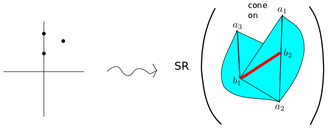
Refer to caption
Figure 2.17: The simplicial complex associated to init​(2,0,1,+0)\textrm{init}(2,0,1,+0). Note that the red edge is the simplicial complex associated to (3,0,0,+0)(3,0,0,+0), the non-R1 locus of (2,0,1,+0)(2,0,1,+0).

We obtain the following consequence of Proposition 2.3.17.

Corollary 2.3.19.

The compatibly split subvarieties of U⟨x,yn⟩U_{\langle x,y^{n}\rangle} listed in Proposition 2.3.17 are Cohen-Macaulay.

Proof.

Each YY described in Proposition 2.3.17 degenerates onto the Stanley-Reisner scheme of a shellable ball. Thus, init​(Y)\textrm{init}(Y) is Cohen-Macaulay. By semicontinuity (of local cohomology), so is YY. ∎

BIBLIOGRAPHY

  • [BB73] A. Białynicki-Birula, Some theorems on actions of algebraic groups, Ann. of Math. (2) 98 (1973), 480–497. MR 0366940 (51 #3186)
  • [BK05] Michel Brion and Shrawan Kumar, Frobenius splitting methods in geometry and representation theory, Progress in Mathematics, vol. 231, Birkhäuser Boston Inc., Boston, MA, 2005. MR 2107324 (2005k:14104)
  • [BP79] Louis J. Billera and J. Scott Provan, A decomposition property for simplicial complexes and its relation to diameters and shellings, Second International Conference on Combinatorial Mathematics (New York, 1978), Ann. New York Acad. Sci., vol. 319, New York Acad. Sci., New York, 1979, pp. 82–85. MR 556009 (81f:52010)
  • [Bri87] Michel Brion, Sur l’image de l’application moment, Séminaire d’algèbre Paul Dubreil et Marie-Paule Malliavin (Paris, 1986), Lecture Notes in Math., vol. 1296, Springer, Berlin, 1987, pp. 177–192. MR 932055 (89i:32062)
  • [Bri99]   , On the general faces of the moment polytope, Internat. Math. Res. Notices (1999), no. 4, 185–201. MR 1677271 (2000i:14068)
  • [Eis95] David Eisenbud, Commutative algebra, Graduate Texts in Mathematics, vol. 150, Springer-Verlag, New York, 1995, With a view toward algebraic geometry. MR 1322960 (97a:13001)
  • [Fog68] John Fogarty, Algebraic families on an algebraic surface, Amer. J. Math 90 (1968), 511–521. MR 0237496 (38 #5778)
  • [Goe] Michael Goemans, Linear programming and polyhedral combinatorics.
  • [Gro67] A. Grothendieck, Éléments de géométrie algébrique. IV. Étude locale des schémas et des morphismes de schémas IV, Inst. Hautes Études Sci. Publ. Math. (1967), no. 32, 361. MR 0238860 (39 #220)
  • [GS] Daniel R. Grayson and Michael E. Stillman, Macaulay2, a software system for research in algebraic geometry, Available at http://www.math.uiuc.edu/Macaulay2/.
  • [Hai98] Mark Haiman, t,qt,q-Catalan numbers and the Hilbert scheme, Discrete Math. 193 (1998), no. 1-3, 201–224, Selected papers in honor of Adriano Garsia (Taormina, 1994). MR 1661369 (2000k:05264)
  • [Hai01]   , Hilbert schemes, polygraphs and the Macdonald positivity conjecture, J. Amer. Math. Soc. 14 (2001), no. 4, 941–1006 (electronic). MR 1839919 (2002c:14008)
  • [Hai04]   , Commutative algebra of nn points in the plane, Trends in commutative algebra, Math. Sci. Res. Inst. Publ., vol. 51, Cambridge Univ. Press, Cambridge, 2004, With an appendix by Ezra Miller, pp. 153–180. MR 2132651 (2006c:14005)
  • [Hoc72] M. Hochster, Rings of invariants of tori, Cohen-Macaulay rings generated by monomials, and polytopes, Ann. of Math. (2) 96 (1972), 318–337. MR 0304376 (46 #3511)
  • [KLS10] Allen Knutson, Thomas Lam, and David E Speyer, Projections of richardson varieties, 2010.
  • [KM09] Shrawan Kumar and Vikram B. Mehta, Finiteness of the number of compatibly split subvarieties, Int. Math. Res. Not. IMRN (2009), no. 19, 3595–3597. MR 2539185 (2010j:13012)
  • [KMY09] Allen Knutson, Ezra Miller, and Alexander Yong, Gröbner geometry of vertex decompositions and of flagged tableaux, J. Reine Angew. Math. 630 (2009), 1–31. MR 2526784 (2010m:13017)
  • [Knu00] Allen Knutson, The symplectic and algebraic geometry of Horn’s problem, Linear Algebra Appl. 319 (2000), no. 1-3, 61–81, Special Issue: Workshop on Geometric and Combinatorial Methods in the Hermitian Sum Spectral Problem (Coimbra, 1999). MR 1799624 (2002g:15051)
  • [Knu04]   , Geometric vertex decompositions, 2004.
  • [Knu09a] Allen Knutson, Compatibly frobenius split subschemes are rigid, 2009.
  • [Knu09b]   , Frobenius splitting, point-counting, and degeneration, 2009.
  • [KS11] Mordechai Katzman and Karl Schwede, An algorithm for computing compatibly frobenius split subvarieties, 2011.
  • [KT01] Shrawan Kumar and Jesper Funch Thomsen, Frobenius splitting of Hilbert schemes of points on surfaces, Math. Ann. 319 (2001), no. 4, 797–808. MR 1825408 (2002d:14004)
  • [Led11] Mathias Lederer, Gröbner strata in the Hilbert scheme of points, J. Commut. Algebra 3 (2011), no. 3, 349–404. MR 2826478
  • [LMP98] V. Lakshmibai, V. B. Mehta, and A. J. Parameswaran, Frobenius splittings and blow-ups, J. Algebra 208 (1998), no. 1, 101–128. MR 1643983 (99i:14059)
  • [MS05] Ezra Miller and Bernd Sturmfels, Combinatorial commutative algebra, Graduate Texts in Mathematics, vol. 227, Springer-Verlag, New York, 2005. MR 2110098 (2006d:13001)
  • [Nak99] Hiraku Nakajima, Lectures on Hilbert schemes of points on surfaces, University Lecture Series, vol. 18, American Mathematical Society, Providence, RI, 1999. MR 1711344 (2001b:14007)
  • [S+] W. A. Stein et al., Sage Mathematics Software, The Sage Development Team, http://www.sagemath.org.
  • [Sch09] Karl Schwede, FF-adjunction, Algebra Number Theory 3 (2009), no. 8, 907–950. MR 2587408 (2011b:14006)
  • [Sja07] Reyer Sjamaar, The moment polytope of a Kähler GG-manifold, Mat. Enseñ. Univ. (N. S.) 15 (2007), no. suppl. 1, 47–58. MR 2417197 (2009j:53112)
  • [Sta96] Richard P. Stanley, Combinatorics and commutative algebra, second ed., Progress in Mathematics, vol. 41, Birkhäuser Boston Inc., Boston, MA, 1996. MR 1453579 (98h:05001)
  • [Tol98] Susan Tolman, Examples of non-Kähler Hamiltonian torus actions, Invent. Math. 131 (1998), no. 2, 299–310. MR 1608575 (2000d:53129)