If we have to points $A$ and $B$ in the Euclidean plane $\mathbb{R}^{2}$, then, as we know from the elementary school, the shortest curve joining $A$ and $B$ is unique and coincides with the straight segment $AB$, so optimal connection problem is trivial in this case. But if we change the way of distance measuring and consider, for example, so-called Manhattan plane, i.e. the plane $\mathbb{R}^{2}$ with fixed standard coordinates $(x,y)$ and the distance function $\rho_{1}(A,B)=|a_{1}-b_{1}|+|a_{2}-b_{2}|$, where $A=(a_{1},a_{2})$ and $B=(b_{1},b_{2})$, then it is not difficult to verify that in this case there are infinitely many shortest curves connecting $A$ and $B$. Namely, if $0\leq a_{1}<b_{1}$ and $0\leq a_{2}<b_{2}$, then any monotonic curve $\gamma(t)=\bigl(x(t),y(t)\bigr)$, $t\in[0,1]$, $\gamma(0)=A$, $\gamma(1)=B$, where functions $x(t)$ and $y(t)$ are monotonic, are the shortest, see Figure 1, left. Another new effect that can be observed in this example is as follows. In the Euclidean plane a curve such that each its sufficiently small piece is a shortest curve joining its ends (so-called locally shortest curve) is a shortest curve itself. In the Manhattan plane it is not so. The length of a locally shortest curve having the form of the letter $\Pi$, see Figure 1, right, can be evidently decreased.

Similar effects can be observed in the surface of standard sphere $S^{2}\subset\mathbb{R}^{3}$. Here the shortest curve joining a pair of points is the lesser arc of the great circle (the cross-section of the sphere by a plane passing through the origin). Two opposite points are connected by infinitely many shortest curves, and if points $A$ and $B$ are not opposite, then the corresponding great circle is unique and it is partitioned into two arcs, both of them are locally shortest, one is the (unique) shortest, but the other one is not. (Really speaking, the difference with the Manhattan plane consists in the fact that for the case of the sphere any directional derivative of the length of any locally shortest arc with respect to its deformation preserving the ends is equal to zero).

Let us consider general situation, when we are given with a finite set $M=\{A_{1},\ldots,A_{n}\}$ of points in a metric space $(X,\rho)$, and we want to connect them in some optimal way in the sense of the total length of the connection. We are working under assumption that we already know how to connect pairs of points in $(X,\rho)$, therefore we need just to organize the set of shortest curves in appropriate way. There are several natural statements of the problem, and we list here the most popular ones.

We start with the Graph Theory problem of finding a minimal spanning tree in a connected weighted graph. It is not difficult to verify that direct enumeration of all possible spanning subtrees of a connected graph leads to an exponential algorithm.

To see that, recall well-known Kirchhoff theorem counting the number of spanning subtrees. If $G=(V,E)$ is a connected graph with enumerated vertex set $V=\{v_{1},\ldots,v_{n}\}$, then its Kirchhoff matrix is defined as $(n\times n)$-matrix $B_{G}=(b_{ij})$ with elements

$$b_{ij}=\left[\begin{array}[]{ll}\deg v_{i}&\quad\text{if $i=j$,}\\ -1&\quad\text{if $\{v_{i},v_{j}\}\in E$,}\\ 0&\quad\text{otherwise.}\end{array}\right.$$

Then the following result based on elementary Graph Theory and Binet–Cauchy formula for determinant calculation is valid, see proof, for example in [4].

Let $G=K_{n}$ be the complete graph with $n$ vertices. Than its Kirchhoff matrix has the following form:

$$B_{K_{n}}=\left(\begin{array}[]{ccccc}n-1&-1&-1&\cdots&-1\\ -1&n-1&-1&\cdots&-1\\ \vdots&\vdots&\vdots&\ddots&\vdots\\ -1&-1&-1&\cdots&n-1\end{array}\right).$$

The algebraic complement of the element $b_{nn}$ is equal to

$$\left|\begin{array}[]{cccc}n-1&-1&\cdots&-1\\ -1&n-1&\cdots&-1\\ \vdots&\vdots&\ddots&\vdots\\ -1&-1&\cdots&n-1\end{array}\right|=\left|\begin{array}[]{ccc}1&\cdots&1\\ -1&\cdots&-1\\ \vdots&\ddots&\vdots\\ -1&\cdots&n-1\end{array}\right|=\left|\begin{array}[]{cccc}1&1&\cdots&1\\ 0&n&\cdots&0\\ \vdots&\vdots&\ddots&\vdots\\ 0&0&\cdots&n\end{array}\right|=n^{n-2},$$

where the first equality is obtained by change of the first row by the sum of all the rows, and the second equality is obtained by change of the $i$th row, $i\geq 2$, by the sum of it with the first row.

Notice that this result is equivalent to Cayley Theorem saying that the total number of trees with $n$ enumerated vertices is equal to $n^{n-2}$.

But it is a surprising fact, that there exist polynomial algorithms constructing minimal spanning trees. Several such algorithms were discovered in 1960s. We tell about Kruskal’s algorithm. Similar Prim’s algorithm can be found in [4].

So, we are given with a connected weighted graph $\bigl(G=(V,E),\omega\bigr)$ with positive weight function $\omega$. At the initial step of Kruckal algorithm we construct the graph $T_{0}=(V,\emptyset)$ and put $E_{0}=E$. If the graph $T_{i-1}$ and the non-empty set $E_{i-1}\subset E$, $i\leq n-1$, have been already constructed, then we choose in $E_{i-1}$ an edge $e_{i}$ of least possible weight and construct a new graph $T_{i}=T_{i-1}\cup e_{i}$ and also a new set $E_{i}=\{e\in E\mid\text{$e\not\in T_{i}$ and $T_{i}\cup e$ is acyclic}\}$. Algorithm stops when the graph $T_{n-1}$ is constructed¹¹ 1 Here the operation of adding an edge $e$ to a graph $G=(V,E)$ can be formally defined as follows: $G\cup e=\left(V,E\cup\{e\}\right)$. Similarly, $G\setminus e=\left(V,E\setminus\{e\}\right)$. .

The set $E_{i}$ is non-empty for all $0\leq i\leq n-2$, because the corresponding subgraphs $T_{i}$ are not connected (the graph $T_{i}$ has $n$ vertices and $i$ edges), therefore all the graphs $T_{1},\ldots,T_{n-1}$ can be constructed. Further, all these graphs are acyclic due to the construction, and $T_{n-1}$ has $n$ vertices and $n-1$ edges, so it is a tree.

To finish the proof it remains to show that the spanning tree $T_{n-1}\subset G$ is minimal. Since the graph ${\cal G}$ has a finite number of spanning trees, a minimal spanning tree does exist. Let $T$ be a minimal spanning tree. We show that it can be reconstructed to the tree $T_{n-1}$ without changing the total weight, so $T_{n-1}$ is also a minimal spanning tree.

To do this, recall that the edges of the tree $T_{n-1}$ are enumerated in accordance with the work of the algorithm. Denote them by $e_{1},\ldots,e_{n-1}$ as above, and assume that $e_{k}$ is the first one that does not belong to $T$. The graph $T\cup e_{k}$ contains a unique cycle $c\supset e_{k}$. This cycle $c$ also contains an edge $e$ not belonging to $T_{n-1}$ (otherwise $c\subset T_{n-1}$, a contradiction). Consider the graph $T^{\prime}=T\cup e_{k}\setminus e$. It is evidently a spanning tree in $G$, and therefore its weight is not less than the weight of the minimal spanning tree $T$, hence

$$\omega(T^{\prime})=\omega(T)+\omega(e_{k})-\omega(e)\geq\omega(T),$$

and thus, $\omega(e_{k})\geq\omega(e)$.

On the other hand, all the edges $e_{1},\ldots,e_{k-1}$ belongs to $T$ by our assumption. Therefore, the graph $T_{k-1}\cup e$ is a subgraph of $T$ and is acyclic, in particular. Hence, $e\in E_{k-1}$ so as $e_{k}\in E_{k-1}$. But the algorithm has chosen $e_{k}$, hence $\omega(e_{k})\leq\omega(e)$. Thus, $\omega(e_{k})=\omega(e)$, and so $\omega(T^{\prime})=\omega(T)$, and therefore $T^{\prime}$ is a minimal spanning tree in ${\cal G}$. But now $T^{\prime}$ contains the edges $e_{1},\ldots,e_{k}$ from $T_{n-1}$. Repeating this procedure we reconstruct $T$ to $T_{n-1}$ in the class of minimal spanning trees. Theorem is proved.

For a connected weighted graph with $n$ vertices and $m$ edges the complexity of the Kruskal’s algorithm can be naturally estimated as $mn\sim n^{3}$. The estimation can be improved to $m\log m\sim n^{2}\log n$. The fastest non-randomized comparison-based algorithm with known complexity belongs to Bernard Chazelle [5]. It turns out that if the weight function is geometrical, then the algorithms can be improved.

Now assume that $M$ is a finite subset of the Euclidean plane $\mathbb{R}^{2}$. It turns out that a minimal spanning tree for $M$ in $\mathbb{R}^{2}$ can be constructed faster than the one for an abstract complete graph with $n=|M|$ vertices by means of some geometrical reasonings. To do that we need to construct so called Voronoi partition of the plane, corresponding to $M$, and the Delaunay graph on $M$. It turns out that any minimal spanning tree for $M$ in $\mathbb{R}^{2}$ is a subgraph of the Delaunay graph, see Figure 3, and the number of edges in this graph is linear with respect to $n$, so the standard Kruskal’s algorithm applied to it gives the complexity $n\log n$ instead of $n^{2}\log n$ for the complete graph with $n$ vertices.

Let us pass to details. Let $M=\{A_{1},\ldots,A_{n}\}\subset\mathbb{R}^{2}$ be a finite subset of the plain. The Voronoi cell of the point $A_{i}$ is defined as

$$\operatorname{Vor}_{M}(A_{i})=\left\{x\in\mathbb{R}^{2}\mid\text{$\|x-A_{i}\|\leq\|x-A_{j}\|$ for all $j$}\right\}.$$

The Voronoi cell for $A_{i}$ is a convex polygonal domain which is equal to the intersection of the closed half-planes restricted by the perpendicular bisectors of the segments $A_{i}A_{j}$, $j\neq i$. It is easy to verify, that the intersection of any two Voronoi cells has no interior points and that $\cup_{i}\operatorname{Vor}_{M}(A_{i})=\mathbb{R}^{2}$. This partition of the plane is referred as Voronoi partition or Voronoi diagram. Two cells $\operatorname{Vor}_{M}(A_{i})$ and $\operatorname{Vor}_{M}(A_{j})$ are said to be adjacent, if there intersection contains a straight segment. The Delaunay graph $D(M)$ is defined as the dual planar graph to the Voronoi diagram. More precisely, the vertex set of $D(M)$ is $M$, and to vertices $A_{i}$ and $A_{j}$ are connected by an edge, if and only if their Voronoi cells $\operatorname{Vor}_{M}(A_{i})$ and $\operatorname{Vor}_{M}(A_{j})$ are adjacent. The edges of the Delaunay graph are the corresponding straight segments.

It is easy to verify, that if the set $M$ is generic in the sense that no three points lie at a common straight line and no four points lie at a common circle, then the Delaunay graph $D(M)$ is a triangulation, i.e. its bounded faces are triangles. In general case some bounded faces could be inscribed polygons. Anyway, the number of edges of the graph $D(M)$ does not exceed $3n$. It remains to prove the following key Lemma.

Let $e=A_{i}A_{j}$ be an edge of a minimal spanning tree $T$ for $M$. We have to show that the Voronoi cells $\operatorname{Vor}_{M}(A_{i})$ and $\operatorname{Vor}_{M}(A_{j})$ are adjacent. The graph $T\setminus e$ consists of two connected components, and this partition generates a partition of the set $M$ into two subsets, say $M_{1}$ and $M_{2}$. Assume that $A_{i}\in M_{1}$ and $A_{j}\in M_{2}$. The minimality of the spanning tree $T$ implies that $\|A_{i},A_{j}\|$ is equal to the distance between the sets $M_{1}$ and $M_{2}$, where $\|A_{i},A_{j}\|$ stands for the distance between $A_{i}$ and $A_{k}$.

By $u$ we denote the middle point of the straight segment $A_{i}A_{j}$, and let $A_{k}$ be another point from $M$. Assume that $A_{k}\in M_{2}$. Due to the previous remark, $\|A_{i},A_{k}\|\geq\|A_{i},A_{j}\|$, therefore

$$\|u,A_{k}\|\geq\|A_{i},A_{k}\|-\|A_{i},u\|\geq\|A_{i}A_{j}\|-\|A_{i},u\|=\|A_{i},A_{j}\|/2=\|u,A_{i}\|=\|u,A_{j}\|.$$

On the other hand, if $\|u,A_{k}\|=\|u,A_{i}\|$, then we have equalities in both above inequalities. The first one means that $u$ lies at the straight segment $A_{i}A_{k}$, hence $A_{k}$ lies at the ray $A_{i}u$. The second equality implies $\|A_{i}A_{k}\|=\|A_{i}A_{j}\|$, and so $A_{k}=A_{j}$, a contradiction. Thus, $\|u,A_{k}\|>\|u,A_{i}\|$, that is $u$ does not belong to the cell $\operatorname{Vor}_{M}(A_{k})$ for $k\not\in\{i,\,j\}$. Thus, $u\in\operatorname{Vor}_{M}(A_{i})\cap\operatorname{Vor}_{M}(A_{j})$,

Since the inequality proved is strict, the same arguments remain valid for points lying close to $u$ on the perpendicular bisector to the segment $A_{i}A_{j}$. Therefore, the intersection of the Voronoi cells $\operatorname{Vor}_{M}(A_{i})$ and $\operatorname{Vor}_{M}(A_{j})$ contains a straight segment, that is the cells are adjacent. Lemma is proved.

The previous arguments work in any dimension. But the trouble is that starting from the dimension $3$ the number of edges in the Delaunay graph need not be linear on the number of its vertices.

The idea that additional forks can help to decrease the length of a connecting network had been already clear to P. Fermat and his students. It seems that Fermat was the first, who stated the following optimization problem: for given three points $A_{1}$, $A_{2}$, and $A_{3}$ in the plane find a point $X$ minimizing the sum of distances from the points $A_{i}$, i.e. minimize the function $F(X)=\sum_{i}\|A_{i},X\|$. For the case when all the angles of the triangle $A_{1}A_{2}A_{3}$ are less than or equal to $120^{\circ}$ the solution was found by E. Torricelli and later by R. Simpson. The construction of Torricelli is as follows, see Figure 4.

On the sides of the triangle $A_{1}A_{2}A_{3}$ construct equilateral triangles $A_{i}A_{j}A^{\prime}_{k}$, $\{i,j,k\}=\{1,2,3\}$, such that they intersect the initial triangle only by the common sides. Then, as Torricelli proved, the circumscribing circles of these three triangles intersect in a point referred as Torricelli point $T$ of the triangle $A_{1}A_{2}A_{3}$. If all the angles $A_{i}$ are less than or equal to $120^{\circ}$, then $T$ lies in the triangle $A_{1}A_{2}A_{3}$ and gives the unique solution to the Fermat problem.²² 2 An elementary proof can be obtained by rotation $R$ of a copy of the triangle around its vertex, say $A_{1}$, by $60^{\circ}$ and considering the polygonal line $L$ joining $A_{2}$, $X$, image $R(X)$ of $X$ under the rotation, and $R(A_{3})$. The length of $L$ is equal to $F(X)$, and minimal value of $F(X)$ corresponds to the location of the $X$ such that $L$ is a straight segment. Later Simpson proved that the straight segments $A_{i}A^{\prime}_{i}$ also pass through the Torricelli point, and the lengths of all these three segments are equal to $F(T)$. If one of the angles, say $A_{3}$, is more than $120^{\circ}$, then the Torricelli point is located outside the triangle and can not be the solution to Fermat problem. In this case the solution is $X=A_{3}$.

So we see, that shortest tree for a triangle in the plane consists of straight segments meeting at the vertices by angles more than or equal to $120^{\circ}$. It turns out, that this $120^{\circ}$-property remains valid in much more general situation.

Let $M=\{A_{1},\ldots,A_{n}\}$ be a finite subset of Euclidean space $\mathbb{R}^{N}$, and $T$ is a Steiner tree connecting $M$. Recall that we defined shortest trees as abstract graphs with vertex set in the ambient metric space. In the case of $\mathbb{R}^{N}$ it is natural to model edges of such graph as straight segments joining corresponding points in the space. The configuration obtained is referred as a geometrical realization of the corresponding graph. Below, speaking about shortest trees in $\mathbb{R}^{N}$ we will usually mean their geometrical realizations. The local structure of a shortest tree (more exactly of a geometrical realization of the tree) can be easily described.

Let $M$ be the vertex set of regular tetrahedron $\Delta$ in $\mathbb{R}^{3}$. Then the network consisting of four straight segments joining the vertices of the tetrahedra with its center $O$ is not a shortest network. Indeed, since $\deg O=4$, then the angles between the edges meeting at $O$ are less than $120^{\circ}$. The set $M$ is connected by three different (but isometrical) shortest networks, each of which has two additional vertices of degree $3$, see Figure 5.

Theorem 3.1 can be just “word-by-word” extended to the case of Riemannian manifolds (we only need to change straight segments by geodesic segments) [1] and even to the case of Alexandrov spaces with bounded curvature. The case of normed spaces turned out to be more complicated (some general results can be found in [2]).

A connected graph $\Gamma$ in $\mathbb{R}^{N}$ (in a Riemannian manifold) whose vertex set contains a finite subset $M\subset\mathbb{R}^{N}$ is called a locally minimal network connecting $M$ or with the boundary $\partial\Gamma=M$, if it satisfies Conditions (1)–(4) from Theorem 3.1. In the case of complete Riemannian manifolds such graphs are minimal “in small,” i.e. the following result holds, see [1].

In the case of normed spaces Theorem 3.3 is not valid even for two-point sets, see example in Figure 1.

Let us return back to the case of Euclidean plane. It turns out that in this case the Torricelli–Simpson construction can be generalized to a geometrical algorithm, that either constructs a locally minimal tree of a given structure for a given boundary set, or reports that such a tree does not exist. This algorithm was discovered by Z. Melzak [9] and improved by F. Hwang [8].

Assume that we are given with a tree $G$ whose vertex degrees are at most $3$, a finite subset $M$ of the plane, and a bijection $\varphi\colon\partial G\to M$, where $\partial G$ is the set of all vertices from $G$ of degrees $1$ and $2$. To start with, partition the tree $G$ into the union of so-called non-degenerate components $G_{i}$ by cutting the tree at each its vertex of degree $2$, see Figure 6. To construct locally minimal network $\Gamma$ of type $G$ spanning $M$ in accordance with $\varphi$ it suffices to construct each its component $\Gamma_{i}$ of type $G_{i}$ on the corresponding boundary $M_{i}=\varphi(\partial G_{i})$, where $\partial G_{i}=\partial G\cap G_{i}$, in accordance with $\varphi_{i}=\varphi|_{\partial G_{i}}$ and to verify the angles between the edges of the components at the vertices of degree $2$. All these angles must be more than or equal to $120^{\circ}$, see Figure 6.

Now we pass to the case of one non-degenerate component, i.e. we assume that $G$ has no vertices of degree $2$ and that $\partial G$ consists of all the vertices of degree $1$. Such trees are referred as binary. If $|\partial G|=2$, then the corresponding locally minimal tree $\Gamma$ is a straight segment. Otherwise, it is easy to verify that each such tree $G$ contains so-called moustaches, i.e. a pair of vertices of degree $1$ neighboring with a common vertex of degree $3$. Fix such moustaches $\{x,x^{\prime}\}\subset\partial G$, by $y$ denote their common vertex of degree $3$, and make a forward step of Melzak algorithm, see Figure 7, that reduces the number of boundary vertices by $1$. Namely, we reconstruct the tree $G$ by deleting the vertices $x$ and $x^{\prime}$ together with the edges $xy$ and $x^{\prime}y$ and adding $y$ to the boundary of new binary tree; reconstruct the set $M$ by deleting the points $\varphi(x)$ and $\varphi(x^{\prime})$ and adding a new point $A_{xx^{\prime}}$ which is the third vertex of a regular triangle constructed on the straight segment $\varphi(x)\varphi(x^{\prime})$ in the plane; and reconstruct the mapping $\varphi$ putting $\varphi(y)=A_{xx^{\prime}}$. Notice that the point $A_{xx^{\prime}}$ can be constructed in two ways, because there are two such regular triangles. Thus, if the number of boundary vertices in the resulting tree is more than $2$, then we can repeat the procedure described above. And if it becomes $2$, then we can construct the corresponding locally minimal tree — the straight segment. Here the forward trace of Melzak algorithm stops. Now we have to reconstruct the initial tree, if possible.

Thus, we have a straight segment $I\subset\mathbb{R}^{2}$ realizing locally minimal tree with unique edge $ab$, and at least one of its ending points has the form $A_{xx^{\prime}}$, where $x$ and $x^{\prime}$ are the boundary vertices of the binary tree $G$ from the previous step, neighboring with their common vertex of degree $3$. Let this common vertex be $a$, that is $a$ corresponds to $A_{xx^{\prime}}$. We reconstruct $G$ by adding edges $ax$ and $ax^{\prime}$. Then we restore the points $\varphi(x)$ and $\varphi(x^{\prime})$ in the plane together with the regular triangle $\varphi(x)\varphi(x^{\prime})A_{xx^{\prime}}$, circumscribe the circle $S^{1}$ around it and consider the intersection of $S^{1}$ with the segment $I$, see Figure 8. If it does not contains a point lying at the smaller arc of $S^{1}$ restricted by $\varphi(x)$ and $\varphi(x^{\prime})$, then the tree $G$ can not be reconstructed and we have to pass to another realization of the forward trace of the algorithm. Otherwise we put $\varphi(a)$ be equal to this point. The straight segments $\varphi(x)\varphi(a)$ and $\varphi(x^{\prime})\varphi(a)$ meet at $\varphi(a)$ by $120^{\circ}$ and together with the subsegment $\varphi(a)\varphi(b)$ form a locally minimal binary tree $\Gamma$ of type $G$ with tree boundary vertices. We repeat this procedure until we either reconstruct the tree of type $G$, or verify all possible realizations of the forward trace and conclude that the tree of type $G$ does not exists.

The Melzak algorithm described above contains an exponential number of possibilities of its forward trace realization, due to two possible locations of each regular triangle constructed by the algorithm. This complexity can be reduced by means of modification suggested by F. Hwang [8]. He showed that considering a bit more complicated configurations of boundary points (four points corresponding to “neighboring moustaches” or three points corresponding to moustaches and “neighboring” degree-$1$ vertex) one always can understand which regular triangle must be chosen, see details in [8].

But unfortunately even a linear time realization of Melzak algorithm does not lead to a polynomial algorithm of a shortest tree finding. The reason is a huge number of possible structures of the tree $G$ with $|\partial G|=n$ together with also exponential number of different mappings $\varphi\colon\partial G\to M$ for fixed $\partial G$ and $M$. Even for binary trees we have $3$ possibilities for $n=4$, see Figure 9, and $15$ possibilities for $n=5$ (notice that the corresponding binary trees are isomorphic as graphs). For $n=6$ we have two non-isomorphic binary trees and the number of possibilities becomes $90$. It can be shown that the total number of possibilities can be estimated by Catalan number and grough exponentially.

So, to obtain an efficient algorithms, we have to find some a priori restrictions on possible structures of minimal networks. In the next subsection we tell about the restrictions generated by geometry of boundary sets.

Here we review our results from [10] and [7]. The goal is to find some restriction on the structure of locally minimal binary trees spanning a given boundary in the plane in terms of geometry of the boundary set. To do this we need to choose or to introduce some characteristics of the network structure and of the boundary geometry.

As a characteristic of the geometry of a boundary set $M$ we take the number of convexity levels $c(M)$. Recall the definition. Let $M$ be a finite non-empty subset of the plane. Take the convex hull $\operatorname{ch}M$ of $M$ and assign the points from $M$ lying at the boundary of the polygon $\operatorname{ch}M$ to the first convexity level $M^{(1)}$ of $M$. If the set $M\setminus M^{(1)}$ is not empty, then define the second convexity level $M^{(2)}$ of $M$ to be equal to the first convexity level of $M\setminus M^{(1)}$, and so on. As a result, we obtain the partition of the set $M$ into its convexity levels, and by $c(M)$ we denote the total number of this levels, see Figure 10.

Now let us pass to definition of a characteristic describing the “complexity” of planar binary trees. Assume that we are given with a planar binary tree $\Gamma$, and let the orientation of the plane be fixed. For any its two edges, say $e_{1}$ and $e_{2}$, we consider the unique path $\gamma$ in $\Gamma$ starting at $e_{1}$ and finishing at $e_{2}$. All interior vertices of $\gamma$ are the vertices of $\Gamma$ having degree $3$. Let us walk from $e_{1}$ to $e_{2}$ along $\gamma$. Then at each interior vertex of $\gamma$ we make either left, or right turn in $\Gamma$. Define the value $\operatorname{tw}(e_{1},e_{2})$ to be equal to the difference between the numbers of left and right turns we have made. In other words, assign to an interior vertex of $\gamma$ the label $\tau=\pm 1$, where $+1$ corresponds to left turns and $-1$ to right turns. Then $\operatorname{tw}(e_{1},e_{2})$ is the sum of these values, see Figure 11. Notice that $\operatorname{tw}(e_{1},e_{2})=-\operatorname{tw}(e_{2},e_{1})$. At last, we put $\operatorname{tw}\Gamma=\max\operatorname{tw}(e_{i},e_{j})$, where the maximum is taken over all ordered pairs of edges of $\Gamma$.

If the tree $\Gamma$ is locally minimal, then the twisting number between any pair of its edges has a simple geometrical interpretation, see Figure 11. Namely, since the angles between any neighboring edges are equal to $2\pi/3$, then $\operatorname{tw}(e_{i},e_{j})$ is equal to the total angle which the oriented edge rotates by passing from $e_{i}$ to $e_{j}$, divided by $\pi/3$.

It turns out, that the twisting number of a locally minimal binary tree with a given boundary is restricted from above by a linear function on the number of convexity levels of the boundary. Namely, the following result holds.

The important particular case $c(M)=1$ corresponds to the vertex sets of convex polygons. Such boundaries are referred as convex.

Notice that the direct statement of Theorem 3.5 is rather easy to prove (it follows from the geometrical interpretation of the twisting number, easy remark that $\operatorname{tw}\Gamma$ always attains at boundary edges, and the monotony of convex polygonal lines). But the converse statement is quite non-trivial. The proof obtained in [7] is based on the complete description of binary trees with twisting number at most five, obtained in terms of so-called triangular tilings that will be discussed in the next subsection.

It turns out that the description of planar binary trees with twisting number at most five can be effectively done in the language of planar triangulations of a special type which are referred as triangular tilings.

The correspondence between diagonal triangulations of planar convex polygons and planar binary trees is well-known: the planar dual graph of such triangulation is a binary tree, see Figure 12, and each binary tree can be obtained in such a way. Here the vertices of the dual graph are centers of the triangles of the triangulation (medians intersection point) and middle points of the sides of the polygon; and edges are straight segments joining either the middle of a side with the center of the same triangle, or two centers of the triangles having a common side.

In the context of locally minimal binary trees, the most effective way to represent the diagonal triangulations is to draw them consisting of regular triangles. Such special triangulations are referred as triangular tilings. The main advantage of the tilings is that the dual binary tree constructed as described above is a locally minimal binary tree with the corresponding boundary. Therefore, tilings “feel the geometry” of locally minimal binary trees and turns out to be very useful in the description of such trees with small twisting numbers.

The main difficulty in constructing a triangulation consisting of regular triangles for a given binary tree is that the resulting polygon can overlap itself. An example of such overlapping can be easily constructed from a binary tree $\Gamma$ corresponding to the diagonal triangulation of a convex $n$-gon, $n\geq 6$, all whose diagonals are incident to a common vertex. But the twisting number of such $\Gamma$ is also at least $6$. The following result is proved in [7].

Theorem 3.7 gives an opportunity to reduce the description of the planar binary trees with twisting number at most five to the description of the corresponding triangular tilings.

To describe all the triangular tilings whose dual binary trees have the twisting number at most five, we decompose each such tiling into elementary “breaks”. The triangles of the tiling are referred as cells. A cell of a tiling $T$ is said to be outer, if two its sides lie at the boundary of $T$ considered as planar polygon. Further, a cell is said to be inner, if no one of its sides lies at the boundary, see Figure 13. An outer cell adjacent to (i.e. intersecting with by a common side) an inner cell is referred as a growth of $T$. A tiling can contains as un-paired growths, so as paired growths, see Figure 14.

For each inner cell we delete exactly one growth adjacent to it, providing such growths exist. As a result, we obtain a decomposition of the initial tiling into its growths and its skeleton (a tiling without growths). Notice, that such a decomposition is not unique.

It turns out that the skeletons of the tilings whose dual binary trees have twisting number at most five can be described easily. Also, the possible location of growthes in such tilings on their skeletons also can be described. The details can be found in [7] or [1]. Here we only formulate the skeletons describing Theorem and include several examples of its application.

Inner cells of a skeleton $S$ are organized into so-called branching points, see Figure 15. After the branching points deleting, the skeleton is partitioned into linear parts. Each linear part contains at most one outer cell. Construct a graph $C(S)$ referred as the code of the skeleton $S$ as follows: the vertex set of $C(S)$ is the set of its branching points and of the outer cells of its linear parts. The edges correspond to the linear parts, see Figure 15.

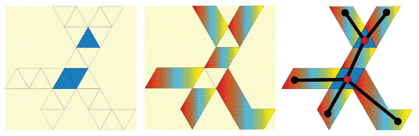
The following result is proved in [7].

All possible codes of such skeletons are depicted in Figure 16.

This description of skeletons and corresponding tilings obtained in [7], was applied to the proof of inverse (non-trivial) statement of Theorem 3.5. In some sense, the proof obtained in [7] is constructive: for each tiling under consideration a corresponding locally minimal binary tree with a convex boundary is constructed.

Another application is a description of all possible binary trees of the skeleton type that can be realized as locally minimal binary trees connecting the vertex set of a regular polygon. It turns out, see details in [1], that there are $2$ infinite families of such trees and $1$ finite family. The representatives of these networks together with the corresponding skeletons are shown in Figure 17.

Let $M$ be a finite subset of a metric space $(X,\rho)$, and assume that $|M|\geq 2$. We put $\operatorname{sr}M=\operatorname{smt}(M)/\operatorname{mst}(M)$. Evidently, $\operatorname{sr}M\leq 1$. The next statement is also easy to prove.

Let $G$ be a Steiner tree connecting $M$. Consider an arbitrary embedding of the graph $G$ into the plane, walk around $G$ in the plane and list consecutive paths forming this tour and joining consecutive boundary vertices from $M$. The length of each such path $\gamma_{PQ}$ joining boundary vertices $PQ$, i.e. the sum of the lengthes of its edges, is more than or equal to the distance $\rho(P,Q)$, due to the triangle inequality. Consider the cyclic path in the complete graph with vertex set $M$ consisting of edges formed by the pairs of consecutive vertices from the tour, and let $T$ be a spanning tree on $M$ contained in this path. It is clear, that $\rho(T)<\sum_{(P,Q)}\rho(\gamma_{PQ})$, where the summation is taken over all the pairs of consecutive vertices of the tour. On the other hand, each edge of the tree $G$ belongs to exactly two such paths, hence $\sum_{(P,Q)}\rho(\gamma_{PQ})=2\rho(G)$. So, we have $\operatorname{sr}(M)\geq\rho(G)/\rho(T)>1/2$. The Assertion is proved.

The value $\operatorname{sr}(M)$ is the relative error appearing under approximation of the length of a shortest tree for a given set $M$ by the length of a minimal spanning tree. The Steiner ratio of a metric space $(X,\rho)$ is defined as the value $\operatorname{sr}(X)=\inf_{M\subset X}\operatorname{sr}(M)$, where the infimum is taken over all finite subsets $M$, $|M|\geq 2$ of the metric space $X$. So, the Steiner ratio of $X$ is the value of the relative error in the worse possible case.

Sometimes, it is convenient to consider so-called Steiner ratios $\operatorname{sr}_{n}(X)$ of degree $n$, where $n\geq 2$ is an integer, which are defined as follows: $\operatorname{sr}_{n}(X)=\inf_{M\subset X,|M|\leq n}\operatorname{sr}(M)$. Evidently, $\operatorname{sr}_{2}(X)=1$. It is also clear that $\operatorname{sr}(X)=\inf_{n}\operatorname{sr}_{n}(X)$.

Steiner ratio was firstly defined for the Euclidean plane in [11], and during the following years the problem of Steiner ratio calculation is one of the most attractive, interesting and difficult problems in geometrical optimization. A short review can be found in [2] and in [12]. One of the most famous stories here is connected with several attempts to prove so-called Gilbert–Pollack Conjecture, see [11], saying that $\operatorname{sr}(\mathbb{R}^{2},\rho_{2})=\sqrt{3}/2$, where $\rho_{2}$ stands for the Euclidean metric, and hence $\operatorname{sr}(\mathbb{R}^{2},\rho_{2})$ is attained at the vertex set of a regular triangle, see Figure 2. In 1990s D. Z. Du and F. K. Hwang announced that they proved the Steiner Ratio Gilbert–Pollak Conjecture [13], and their proof was published in Algorithmica [14]. In spite of the appealing ideas of the paper, the questions concerning the proof appeared just after the publication, because the text did not appear formal. And about 2003–2005 it becomes clear that the gaps in the D. Z. Du and F. K. Hwang work are too deep and can not be repaired, see detail in [15].

Gilbert and Pollack calculated $\operatorname{sr}_{3}(\mathbb{R}^{2},\rho_{2})$ in their paper [11]. We include their proof here.

Since the Steiner ratio of a regular triangle is equal to $\sqrt{3}/2$, then $\operatorname{sr}_{3}(\mathbb{R}^{2},\rho_{2})\leq\sqrt{3}/2$, so we just need to prove the opposite inequality. To do this, consider a triangle $ABC$ in the plane. If one of its angles is more than or equal to $120^{\circ}$, then the shortest tree coincides with minimal spanning tree, so in this case $\operatorname{sr}(ABC)=1$. So it suffices to consider the case when all the angles of the triangle are less than $120^{\circ}$.

Let $S$ be the Torricelli point of the triangle $ABC$. Show firstly that $|AS|\leq|BS|$, if and only if $|BC|\geq|AC|$, i.e. the shortest edge of the Steiner minimal tree lies opposite with the longest side of the triangle. The proof is shown in Figure 18, left. Indeed, if $|BS|<|AS|$, then we take the point $B^{\prime}\in[S,B]$ with $|SB^{\prime}|=|SA|$, hence $|CB^{\prime}|=|CA|$ due to symmetry and $|CB^{\prime}|<|CB|$ because $B^{\prime}\geq 120^{c}$. Conversely, if $|BC|>|B^{\prime}C|$, then there exists $B^{\prime}\in[B,S]$ with $|CB^{\prime}|=|CA|$, because $|BC|>|CA|>|SC|$. Then $|AS|=|SB^{\prime}|<|SB|$.

Thus, the two-edges tree $T=[A,B]\cup[B,C]$ is a minimal spanning tree for $ABC$, if and only if $BC$ is the longest side of $ABC$, if and only if $|AS|\leq|BS|$ and $|AS|\leq|CS|$. Consider the points $E\in[B,S]$ and $D\in[C,S]$, such that $|AS|=|ES|=|DS|$, and put $x=|AC|$, $y=|AB|$, $z=|DE|=|AD|=|AE|$, and $x^{\prime}=|CD|$, $y^{\prime}=|EB|$. Then $|SA|=|SE|=|SD|=z/\sqrt{3}$ and

$$\operatorname{smt}(M)=3|SA|+|DC|+|EB|=\sqrt{3}z+x^{\prime}+y^{\prime}\qquad\text{and}\qquad\operatorname{mst}(M)=x+y,$$

where $M$ stands for the set $\{A,B,C\}$. But $x\leq x^{\prime}+z$ and $y\leq y^{\prime}+z$, due to the triangle inequality, and hence

$$\operatorname{sr}(M)=\frac{\sqrt{3}z+x^{\prime}+y^{\prime}}{x+y}\geq\frac{\sqrt{3}z+x^{\prime}+y^{\prime}}{x^{\prime}+z+y^{\prime}+z}=\frac{\sqrt{3}z+x^{\prime}+y^{\prime}}{x^{\prime}+y^{\prime}+2z}\geq\frac{\sqrt{3}}{2}.$$

Thus, we proved the following statement.

For small $n$ it is already proved that $\operatorname{sr}_{n}(\mathbb{R}^{2},\rho_{2})=\sqrt{3}/2$ (recently O. de Wet proved it for $n\leq 7$, see [16]). The proof of de Wet is based on the analysis of Du and Hwand method from [14] and understanding that it works for boundary sets with $n\leq 7$ points. Also in 60th several lower bounds for $\operatorname{sr}(\mathbb{R}^{2},\rho_{2})$ were obtained, and the best of them is worse than $\sqrt{3}/2$ in the third digit only.

The following result is evident, but useful.

This implies, that $\operatorname{sr}(\mathbb{R}^{n},\rho_{2})\leq\operatorname{sr}(\mathbb{R}^{2},\rho_{2})\leq\sqrt{3}/2$. Recall that Gilbert–Pollack conjecture implies that the Steiner ratio of Euclidean plane attains at the vertex set of a regular triangle. In multidimensional case the situation is more complicated. The following result was obtained by Du and Smith [17]

Consider the boundary set $P$ in $\mathbb{R}^{n+1}$, consisting of the following $1+n(n+1)$ points: one point $(0,\ldots,0)$ and $n(n+1)$ points all whose coordinates except two are zero, one is equal to $1$, and the remaining one is $-1$. It is clear that $P$ is a subset of $n$-dimensional plane defined by the next linear condition: sum of all coordinates is equal to zero. Represent $P$ as the union of the subsets $P^{i}=\{x\in P\mid x^{i}=1\}\cup\{(0,\ldots,0)\}$. Notice that each set $P^{i}$, $i=1,\ldots,n+1$, consists of $n+1$ points and forms the vertex set of an regular $n$-dimensional simplex (to see that it suffices to verify that all the distances between the pairs of points from $P^{i}$ are the same and are equal to $\sqrt{2}$). The configuration of $7$ points in $\mathbb{R}^{3}$ is shown in Figure 19 (this case is not important for us, but it is easy to draw). Now, $\operatorname{mst}(P)=(n+1)\operatorname{mst}(P^{i})$, but for $n\geq 3$ we conclude that $\operatorname{smt}(P)<(n+1)\operatorname{smt}(P^{i})$, because the degree of the vertex $(0,\ldots,0)$ in the corresponding network which is the union of the shortest networks for $P^{i}$ is equal to $n+1\geq 4$ that is impossible in the shortest network due to the Local Structure Theorem 3.1. So,

$$\operatorname{sr}(P)=\operatorname{smt}(P)/\operatorname{mst}(P)<\frac{(n+1)\operatorname{smt}(P^{i})}{(n+1)\operatorname{mst}(P^{i})}=\operatorname{sr}(P^{i}).$$

References

- [1] A. O. Ivanov, and A. A. Tuzhilin. Branching Solutions to One-Dimensional Variational Problems. Singapore, New Jersey, London, Hong Kong, 2001. 342 p.
- [2] A. O. Ivanov, and A. A. Tuzhilin. Extreme Networks Theory. Moscow, Izhevsk, 2003. 406 p. [In Russian.]
- [3] A. O. Ivanov, and A. A. Tuzhilin. One-dimensional Gromov minimal filling problem. // Sbornik: Mathematics. 2012. V. 203, No 5. P. 677-726 [Matem. sb. 2012. T. 203, No 5. S. 65-118].
- [4] V. A. Emelichev, at al. Lections on Graph Theory. Moscow, 1990. 384 p. [In Russian.]
- [5] B. Chazelle. The soft heap: an approximate priority queue with optimal error rate. // Journal of the Association for Computing Machinery. 2000. V. 47, No 6. P. 1012-1027.
- [6] A. O. Ivanov and A. A. Tuzhilin. The geometry of inner spanning trees for planar polygons. // Izvestiya: Mathematics. 2012. V. 76, No 2. P. 215–244 [Izv. RAN. Ser. Matem. 2012. T. 76, No 2. S. 3-36].
- [7] A. O. Ivanov and A. A. Tuzhilin. The Steiner problem in the plane or in plane minimal nets.// Mathematics of the USSR-Sbornik. 1993. V. 74, No 2. P. 555–582 [Matem. Sb. 1991. T. 182, No 12. S. 1813-1844].
- [8] F. K. Hwang. A linear time algorithm for full Steiner trees. // Oper. Res. Letter. 1986. V. 5. P. 235–237.
- [9] Z. A. Melzak. On the problem of Steiner. // Canad. Math. Bull. 1960. V. 4. P. 143–148.
- [10] A. O. Ivanov and A. A. Tuzhilin. Solution of the Steiner problem for convex boundaries. // Russian Mathematical Surveys. 1990. V. 45, No 2. P. 214-215 [Uspekhi Matem. Nauk. 1990. T. 45, No 2(272). S. 207-208].
- [11] E. N. Gilbert and H..O. Pollak. “Steiner minimaltrees.” // SIAM J. Appl. Math. 1968. V. 16, No 1. P. 1–29.
- [12] D. Cieslik. The Steiner ratio. Springer, 2001. 256 p.
- [13] D. Z. Du, F. K. Hwang. The Steiner ratio conjecture of Gilbert–Pollak is true. // Proc. Nat. Acad. Sci. 1990. V. 87. P. 9464–9466.
- [14] D. Z. Du, F. K. Hwang. A proof of Gilbert–Pollak Conjecture on the Steiner ratio. // Algorithmica. 1992. V. 7. P. 121–135.
- [15] A. O. Ivanov and A. A. Tuzhilin. The Steiner Ratio GilbertPollak Conjecture Is Still Open. Clarification Statement. // Algorithmica. 2012. V. 62. No 1–2. P. 630–632.
- [16] P. O. de Wet. Geometric Steiner Minimal Trees. PhD Thesis. UNISA, Pretoria, 2008.
- [17] D. Z. Du and W. D. Smith. Disproofs of Generailzed Gilbert–Pollack conjecture on the Steiner ratio in three and more dimensions. // Combin. Theory. 1996. V. 74. Ser. A. P. 115–130.
- [18] W. D. Smith and J. M. Smith. On the Steiner ratio in -Space. // J. of Comb. Theory. 1995. V. 65. Ser. A. P. 301–322.
- [19] R. L. Graham and F. K. Hwang. A remark on Steiner minimal trees. // Bull. of the Inst. of Math. Ac. Sinica. 1976. V. 4. P. 177–182.
- [20] N. Innami and B. H. Kim. Steiner ratio for Hyperbolic surfaces. // Proc. Japan Acad. 2006. V. 82. Ser. A. No 6. P. 77–79.
- [21] D. Cieslik, A. Ivanov and A. Tuzhilin. Steiner Ratio for Manifolds. // Mat. Zametki. 2003. V. 74. No 3. P. 387-395 [Mathematical Notes. 2003. V. 74. No 3. P. 367-374].
- [22] M. Gromov. Filling Riemannian manifolds. // J. Diff. Geom. 1983. V. 18. No 1. P. 1–147.
- [23] A. O. Ivanov, A. A. Tuzhilin. Steiner Ratio. The State of the Art. // Matemat. Voprosy Kibern. 2002. V. 11. P. 27–48 [In Russian].
- [24] P A. Borodin. An example of nonexistence of a steiner point in a Banach space. // Matem. Zametki. 2010. V. 87. No 4. P. 514–518 [Mathematical Notes. 2010. V. 87. No 4. P. 485-488].
- [25] A. O. Ivanov, Z. N. Ovsyannikov, N. P. Strelkova, A. A. Tuzhilin. One-dimensional minimal fillings with edges of negative weight. // Vestnik MGU, ser. Mat., Mekh. 2012. No 5. P. 3–8.
- [26] A. Yu. Eremin. Formula calculating the weight of minimal filling. // Matem. Sbornik. 2012. [To appear].
- [27] Z. N. Ovsyannikov. Pseudo-additive metric spaces and minimal fillings. // Vestnik MGU. 2013. [To appear].
- [28] K. A. Zareckii. Constructing a tree on the basis of a set of distances between the hanging vertices. // Uspehi Mat. Nauk. 1965. V. 20. No 6. P. 90-92. [In Russian].
- [29] J. M. S. Simões-Pereira. A note on the tree realizability of a distance matrix. // J. Combinatorial Th. 1969. V. 6. P. 303–310.
- [30] E. A. Smolenskij. About a Linear Denotation of Graphs. // J. vych. matem. i matem. phys. 1962. V. 2. No 2. P. 371–372. [In Russian].
- [31] S. L. Hakimi, S. S. Yau. Distane matrix of a graph and its realizability. // Quart. Appl. Math. 1975. V. 12. P. 305–317.
- [32] O. V. Rubleva. Additivity Criterion for finite metric spaces and minimal fillings. // Vestnik MGU, ser. matem., mekh. 2012. No 2. P. 8–11.
- [33] M. Gromov. Hyperbolic groups. // in book: S. M. Gersten, ed. Essays in Group Theory. 1987. Springer.
- [34] E. I. Filonenko. Degree Steiner subratio of Euclidean plane. // Vestnik MGU, ser. matem., mekh. 2013. To appear.
- [35] A. S. Pakhomova. Estimates for Steiner–Gromov ratio and Steiner subratio. // Vestnik MGU, ser. matem., mekh. 2013. To appear.
- [36] Z. N. Ovsyannikov. Steiner ratio, Steiner–Gromov ratio and Steiner subratio for the metric space of all compact subsets of the Euclidean space with Hausdorff metric. // Vestnik MGU, ser. matem., mekh. 2013. To appear.