Uncertainty Relations and Indistinguishable Particles

Quantum theory imposes fundamental limitations on our ability to simultaneously predict the outputs of measurements of different observables¹¹ 1 A closely related subject is that of fundamental limitations quantum theory imposes on our ability to perform simultaneous non-demolition measurements of different observables.. This observation was formalised by the Uncertainty Principle [1, 2], which has played a pivotal role in the conceptual clarification of quantum theory. It also plays an important role in quantum information theory and cryptography [3, 4, 5, 6, 7].

Most of the analysis of uncertainty relations is done within the framework of distinguishable particles, important exceptions being the analysis of Bohr and Rosenfeld [8] and the work of Glauber [9]. These exceptions explore uncertainty relations for field observables such as components of the electric and magnetic field and mode quadratures. The central goal of this paper is to derive and understand uncertainty relations for measurements of particle quantum numbers (q-numbers) on multi-particle states. Naively one may expect uncertainty relations for single particle states to extrapolate in a simple way. Is this true? Does a conventional understanding of single particle uncertainty relations ever break down for multi-particle states?

Consider two q-numbers $\mathcal{A}$ and $\mathcal{B}$ for a particle, each with (finite) $n$ mutually exclusive possible outcomes. Consider the corresponding observables which we represent by operators $A_{1}$ and $B_{1}$ in an $n$-dimensional Hilbert space $\mathcal{H}$. Let $\left\{\ket{i}\right\}$ and $\left\{\ket{\bar{j}}\right\}$ be the complete bases of eigenstates of $A_{1}$ and $B_{1}$ respectively. A good measure of the uncertainty of an observable is the Shannon entropy of its probability distribution. For a pure state $\ket{\psi}\in\mathcal{H}$, the Shannon entropies for $\mathcal{A}$ and $\mathcal{B}$ are given by

where $P_{i}(A_{1};\psi):=\left|\braket{i|\psi}\right|^{2}$, $P_{j}(B_{1};\psi):=\left|\braket{\bar{j}|\psi}\right|^{2}$, and the units are in nats (which we use throughout the paper). Note the maximum value of a Shannon entropy is given when one has a constant probability distribution, i.e., $H(A_{1};\psi)$ and $H(B_{1};\psi)\leq\ln n$.

The sum of these Shannon entropies is constrained by the uncertainty relation [10, 11]:

where

By definition, $c$ is bounded: $0\leq c\leq 1$. As Shannon entropies for discrete probability distributions are positive definite, for observables with $c<1$, relation (3) implies at least one of the entropies must be non-zero.

We have characterized relation (3) for operators $A_{1}$ and $B_{1}$, which refer to particle q-numbers. However, the result applies to any $s$-outcome operators acting on an $s$-dimensional Hilbert space $\mathcal{H}$ where $s\in\mathbb{N}$. We can therefore apply (3) to multi-particle states. The distinguishability of particle ordering becomes important when one considers more than 1 particle. Does an extension of (3) to multi-particle states depend on whether one considers distinguishable or indistinguishable particles?

Consider $N$ distinguishable particles. There are $n$ possible outcomes for each particle, giving us $n^{N}$ possible outcomes in total. Let $A^{(i)}$ be the operator representing the q-number $\mathcal{A}$ for the $i$^th particle with a basis of eigenstates $\{\smash{\ket{m}}_{i}\}$ such that

where $\ket{m}_{i}\in\mathcal{H}_{i}$ and $\mathcal{H}_{i}$ is the Hilbert space for the $i$^th particle. The $N$-particle state $\ket{\psi_{N}}$ is then an element of $\bigotimes^{N}_{i=1}\mathcal{H}_{i}$. Define a new observable whose eigenstates correspond to the distinct outcomes of a measurement of $\mathcal{A}$ on the system, where the measurement can distinguish particle ordering:

where the eigenvalues $e_{m_{1}\cdots m_{N}}$ are chosen to be non-degenerate. Then for an $N$-particle state $\ket{\psi_{N}}$, the Shannon entropy of $\mathcal{A}$ is given by

where $P_{i_{1}\ldots i_{N}}(A_{N};\psi_{N})=|_{1}\!\smash{\bra{i_{1}}}\cdots_{N}\!\smash{\bra{i_{N}}}{\psi_{N}}\rangle|^{2}$.

Note that $H(A_{N};\psi_{N})$ is the joint Shannon entropy for the outcomes of $A^{(i)}$ for each particle. Define an analogous observable and entropy for $\mathcal{B}$. Utilizing relation (3) but replacing $A_{1}$ with $A_{N}$ and $B_{1}$ with $B_{N}$, one finds an entropic uncertainty relation

where $c$ is defined as in Eq. (4).

This result is easily understood for cases where $\ket{\psi_{N}}$ is unentangled:

The average information gained about $A_{N}$ over the ensemble equals the sum of the average information gained about $A^{(i)}$ for each particle:

Then,

which gives the same bound on $H(A_{N};\psi_{N})+H(B_{N};\psi_{N})$ as relation (8) for the special case where $\ket{\psi_{N}}$ is unentangled.

Relation (11) highlights an interesting feature of relation (8); that it is unaffected by possible entanglement of $\ket{\psi_{N}}$. It is not immediately obvious to us why this is the case. Our thoughts go as follows:

1. (a)

   The state of particle ‘$i$’, $\rho^{(i)}=\mathop{\textrm{tr}}_{\neq i}[\ket{\psi_{N}}\bra{\psi_{N}}]$, can become mixed, i.e. the von Neumann entropy $S(\rho^{(i)})=-\mathop{\textrm{tr}}[\rho^{(i)}\ln\rho^{(i)}]>0$. A non-zero $S(\rho^{(i)})$ constrains the Shannon entropy of $\mathcal{A}$ and $\mathcal{B}$ for particle ‘$i$’ [12, 13]:

   $$\left.\begin{array}[]{c}H(A^{(i)},\rho^{(i)})\\[1.42262pt] H(B^{(i)},\rho^{(i)})\end{array}\right\}\geq S(\rho^{(i)})\,.$$

   (12)

   This suggests it may be difficult for entangled states to saturate the bound (8).

2. (b)

   The subadditivity of the Shannon entropy implies

   $$H(A_{N},\psi_{N})<\sum_{i=1}^{N}H(A^{(i)},\rho^{(i)}),$$

   (13)

   for correlated observables $A^{(i)}$, and similarly for $\mathcal{B}$. This disallows a direct use of our previous observation in explaining why entangled states cannot overcome relation (11).

The salient feature of both relations (8) and (11) is the proportionality to $N$ of the lower bounds. We claim that this feature is indicative of the assumption that it is possible to define probabilities for the outcomes of measurements of q-numbers $\mathcal{A}$ and $\mathcal{B}$ for each particle.

It is well known [11] that, for a given quantum state, relation (3) is not necessarily the strongest possible bound. Accordingly, neither are relations (8) and (11).

To compare uncertainties of particle q-numbers for distinguishable and indistinguishable particles, we have to be careful about the precise meaning of the probabilities of the various outcomes for multi-particle states.

For distinguishable particles, the meaning is simple. For a 2 particle state we can consider observables for each particle $\mathcal{O}^{(1)}$ and $\mathcal{O}^{(2)}$ such that

This defines the natural tensor product decomposition $\mathcal{H}_{1}\otimes\mathcal{H}_{2}$ where $\mathcal{H}_{i}$ corresponds to the $i$-th particle. Suppose we have a state $\rho$ which is pure and unentangled

where $\smash{\ket{\psi^{(1)}}}_{\!1}\in\mathcal{H}_{1}$ and $\smash{\ket{\psi^{(2)}}}_{\!2}\in\mathcal{H}_{2}$. Let $\mathcal{O}^{(1)}$ and $\mathcal{O}^{(2)}$ be position projectors for positions $x_{1}$ and $x_{2}$ respectively, then

which is the probability for particle 1 to be measured at $x_{1}$ and particle 2 to be measured at $x_{2}$.

Consider indistinguishable particles. Now all observables commute with permutations of the particle states i.e., for a permutation operator $P_{1\leftrightarrow 2}$ that permutes the states in $\mathcal{H}_{1}$ and $\mathcal{H}_{2}$ and any observable $\mathcal{O}$,

This defines a superselection rule to constrain direct measurements to irreducible representations of the permutation group i.e., symmetric and anti-symmetric under $P_{1\leftrightarrow 2}$.

Importantly for our considerations, the constraint (17) means all observables must act non-locally on the tensor product decomposition²² 2 So the Fock space is a much better decomposition for the states. $\mathcal{H}_{1}\otimes\mathcal{H}_{2}$. The observable which then corresponds closest to $\mathcal{O}^{(1)}\mathcal{O}^{(2)}=\smash{\ket{x_{1}}}_{\!1}{}_{1}\!\smash{\bra{x_{1}}}\otimes\smash{\ket{x_{2}}}_{\!2}{}_{2}\!\smash{\bra{x_{2}}}$ is then,

with $+$ or $-$ corresponding to bosons or fermions respectively. The expectation value of this observable gives us the probability that we shall measure a particle at $x_{1}$ and another at $x_{2}$.

The probabilities given by $\langle\mathcal{O}^{(1)}\mathcal{O}^{(2)}\rangle$ and $\langle\mathcal{O}^{(12)}\rangle$ have fundamentally different meanings. Predictions for distinguishable particles are counterfactual [14] because they assume the existence of particle labels that cannot be measured.

The probabilities and hence Shannon entropies in relation (3) are given physical meaning by the standard axioms of quantum theory that the outcomes of a measurement (eigenstates of an observable) correspond to outputs of a measuring apparatus with probabilities for occurrence defined in the normal way. What is of physical interest are these outputs. We assume:

1. (a)

   An ideal apparatus whose outputs are in one-to-one correspondence with the outcomes.

2. (b)

   Meaningful probabilities can be defined for these outcomes.

Then a Shannon entropy can be defined on the probability distribution of the outputs. Assumption (a) ensures direct usefulness to physics. This Shannon entropy of the outputs rather than the outcomes (eigenstates of some observable) can then be used to compare different theories whose probabilities have very different meanings.

Suppose we perform measurements of q-numbers $\mathcal{A}$ and $\mathcal{B}$ on an infinite, homogeneous ensemble of pure $N$-particle states. Define the Shannon entropy of the outputs of the measurement apparatus as $H_{N}(\mathcal{A})$ and $H_{N}(\mathcal{B})$ for measurements of $\mathcal{A}$ and $\mathcal{B}$, respectively.

Identifying the outputs with outcomes for measurements of $N$ distinguishable particles gives us,

and similarly for $\mathcal{B}$.

For the outputs of measurements of $\mathcal{A}$ and $\mathcal{B}$ over $N$-particle states we can write

where $\chi_{\textrm{min}}(N;\mathcal{A},\mathcal{B})$ is the real minimum over the $N$-particle Hilbert space. In this context, the uncertainty relation for distinguishable particles gives

We now define $H_{N}(\mathcal{A})$ and $H_{N}(\mathcal{B})$ for $N$-particle states of indistinguishable particles.

In order to define $H_{N}(\mathcal{A})$, the type of measurement interaction must be considered. Consider particles with two compatible q-numbers $\mathcal{A}$ and $\mathcal{C}$, with eigenmodes $\alpha_{i}$ and $c_{j}$ respectively. Let $m$ be the number of $\mathcal{C}$ eigenmodes and consider the case where $m>n$. The two-particle states $\ket{\alpha_{1},c_{1};\alpha_{2},c_{2}}$ and $\ket{\alpha_{2},c_{1};\alpha_{1},c_{2}}$ are reliably distinguishable in an experiment measuring $\mathcal{A}$ if the interaction also couples to modes of $\mathcal{C}$. The modes of $\mathcal{C}$ then act as a reference frame [15, 16, 17, 18, 19] for the effective ordering distinguishability of the particles.

As an example, $\mathcal{C}$ may relate to the position of the particle. Measurements can then distinguish particle ordering if the measurement interaction has position dependence, such as the magnetic field in a Stern-Gerlach experiment being localized in space.

For an $N$-particle state, the $n^{N}$ possible outputs we have for distinguishable particles correspond³³ 3 This correspondence can be given by the isomorphism $f_{\chi}$ defined in [20]. to indistinguishable particle states where the modes of $\mathcal{C}$ are different for each particle and also fixed over the set of outputs. These states—where the modes of $\mathcal{C}$ are different for each particle—form only a subspace of the $N$-particle states for indistinguishable particles. It is not guaranteed that the other $N$-particle states satisfy the same bounds for $H_{N}(\mathcal{A})+H_{N}(\mathcal{B})$.

We require the states of distinguishable particles to correspond to states of indistinguishable particles with modes of $\mathcal{C}$ fixed for the following reasons. With distinguishable particles, for states that are elements of $\otimes_{i=1}^{N}\mathcal{H}_{i}$ and measurements of $\mathcal{A}$ or $\mathcal{B}$, it doesn’t matter what the q-number $\mathcal{A}$ is referenced to. With indistinguishable particles where the reference mode $\mathcal{C}$ is modelled, different reference modes are distinguished; i.e., the states $|\alpha_{1},c_{1};\alpha_{2},c_{2}\rangle$ and $|\alpha_{1},c_{3};\alpha_{2},c_{4}\rangle$ are different but give equivalent probabilities for $\mathcal{A}$ and $\mathcal{B}$. Thus they can be identified with the same state $|1\rangle_{1}|2\rangle_{2}$.

Consider particle creation operators $a^{\dagger}_{jl}$ (fermionic or bosonic) which create a particle in mode ‘$j$’ for $\mathcal{A}$ and mode ‘$l$’ for $\mathcal{C}$ such that the state $a^{\dagger}_{jl}\ket{0}$ (where $\ket{0}$ is the Fock vacuum) corresponds⁴⁴ 4 They are equivalent in terms of giving the same probabilities for particle q-numbers. The Fock space however, allows for measurements of q-numbers which are impossible for a quantum theory with distinguishable particles, i.e., superpositions of occupation number eigenstates. to the $A_{1}$ eigenstate $\ket{j,l}_{1}$. One can also define ladder operators $\bar{a}^{\dagger}_{il}$ such that $\bar{a}^{\dagger}_{il}\ket{0}$ corresponds to an eigenstate of $B_{1}$, $\ket{\bar{i},l}_{1}$. The two sets of operators are related by the Bogoliubov transformation

For $N$-particle states of indistinguishable particles, the Shannon entropy of the outcomes of $\mathcal{A}$ is constructed in the following way. Define the observable

where $\delta_{(\sum_{b,c}i_{bc})N}$ is a Kronecker delta. The eigenvalues $f_{i_{1}\cdots i_{n}}$ are, chosen to be non-degenerate and the ordering of the ladder operators arbitrary. (The ordering of ladder operators does not affect any result of this paper. In cases where the ordering isn’t specified, the reader is free to choose it.) Then the corresponding Shannon entropy is

where

Identifying outputs to outcomes gives us

for a state of $N$ indistinguishable particles $\ket{\phi}$ and an apparatus that couples to $\mathcal{A}$ and $\mathcal{C}$. An analogous entropy for B can also be defined with an observable $B_{N|C}$ which is given by $A_{N|C}$ with the ladder operators $a^{\dagger}_{jl}$ replaced by $\bar{a}^{\dagger}_{jl}$.

We are now in a position to construct an uncertainty relation for $H_{N}(\mathcal{A})$ and $H_{N}(\mathcal{B})$. We choose the Hilbert space to be the $N$-particle subspace of the entire Fock space of these modes. Applying relation (3) to $A_{N|C}$ and $B_{N|C}$ instead of $A_{1}$ and $B_{1}$, we obtain

where

So how does (27) compare to (21)? Firstly, a sanity check. If we restrict ourselves to an $N$-particle subspace where the modes of $\mathcal{C}$ are different for each particle and also fixed, the outcomes and probabilities of a measurement of $\mathcal{A}$ or $\mathcal{B}$ should be in one-to-one correspondence with the distinguishable particles case. Thus, with this restriction, $H(A_{N|C};\psi)+H(B_{N|C};\psi)$ should never be smaller than $-2N\ln c$. We can compute the RHS of (27) with this restriction. The overlap between eigenstates of $A_{N|C}$ and $B_{N|C}$ can be given without loss of generality by

Thus with this restricted subspace,

which agrees with relation (8).

For the full $N$-particle Hilbert space, relation (27) can be written explicitly in terms of $U_{ij}$. Denote $P_{N}$ as the group of permutations of the components of the elements of $\mathbb{N}^{N}$. For example, let $\tilde{k}=(k_{1},\cdots,k_{N})\in\mathbb{N}^{N}$ and $\sigma\in P_{N}$ such that $\sigma$ swaps the first and second components:

Define

and

where $k_{i},t_{i}\leq n$ and $l_{i}\leq m$. Also define

Then for bosons and fermions respectively, relation (27) gives us

and

We can immediately compare these uncertainty relations to Eq. (21). Eq. (21) has two nice properties. Firstly, it is proportional to $N$. Secondly, different choices of $\cal A$ and $\cal B$ affect only the slope of this proportionality. In contrast, the euations above for bosons and fermions cannot be expected to have these properties. This is because they involve sums of $V(\tilde{k},\tilde{t})$ which generally are complex numbers and thus generally interfere with each other.

Can we say anything general about the N dependence of $\chi^{\mathrm{boson}}_{\mathrm{min}}$ and $\chi^{\mathrm{ferm}}_{\mathrm{min}}$? Surprisingly we can. In the next two sections we derive upper bounds on them, dependent only on $N$ and $n$.

Let us focus on states that do not correspond to states of distinguishable particles. Any interesting differences between (36) and (21) are likely to show up in this region of the Hilbert space. Consider for instance an $N$-boson eigenstate of $A_{N|C}$ where every particle is in the same $\mathcal{C}$ eigenmode ‘$l$’:

By construction, $H(A_{N|C};\omega)=0$. An upper bound can be found for $H(B_{N|C};\omega)$ using the following argument:

The Bogoliubov transformation (22) does not change (a) the number of particles, and (b) the $\mathcal{C}$ eigenmodes. Each component of $\ket{\omega}$ in the $\mathcal{B}$-mode basis must have $N$-particles where each particle is still in $\mathcal{C}$ eigenmode ‘$l$’. How many possible components with these properties are there? The question is isomorphic to the question, “how many ways can I place $N$ indistinguishable balls into $n$ distinguishable boxes?” The answer [21] is $\binom{N+n-1}{N}$. Thus,

For $N\geq n$,

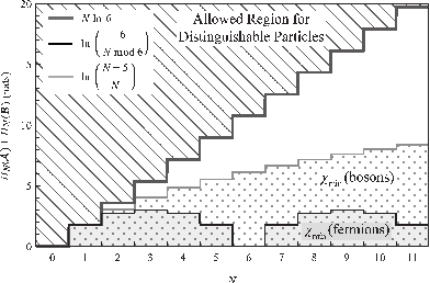
and hence this upper bound is of order $\ln N$, which shows that Eq. (36), unlike Eq. (21), cannot be proportional to $N$.

Relation (40) provides an upper bound on $\chi_{\textrm{min}}$

which is dependent only on $N$ and $n$. This is demonstrated in Fig. 1.

To illustrate relation (42), consider an $N=2=n$ example with photons, given by the $A_{2|C}$ eigenstate

where 1 and 2 denote polarization eigenmodes of $\mathcal{A}$ and $k$ denotes an eigenmode of $\mathcal{C}$. The q-number $\mathcal{C}$ could be for instance position, momentum, or a combination of angular momentum q-numbers. Choose eigenmodes of $\mathcal{B}$ as rotations of 1 and 2 through an angle $\alpha$,

such that

Suppose $\mathcal{B}$ is complementary to $\mathcal{A}$, i.e. $\alpha=\pi/4$; then,

which is smaller than the RHS of (42) and half the lower bound (21) for $H_{N}(\mathcal{A})+H_{N}(\mathcal{B})$ with distinguishable particles. Interestingly, the upper bound (42) can be saturated for $\alpha=\frac{1}{2}\arctan\sqrt{2}$ where $\mathcal{B}$ is not complementary to $\mathcal{A}$:

Let’s turn our attention to fermions, whose ladder operators we shall denote by $b_{jl}$ and $b^{\dagger}_{jl}$. For the case $N=n$, the RHS of Eq. (37) can be computed in the following way. Consider the state

which is an eigenstate of $A_{n|C}$. Rewriting the state in terms of modes of $\mathcal{B}$ gives

where we also used the fact that $\ket{0}$ is invariant under Bogoliubov transformations (22) that do not mix creation and annihilation operators. Thus

which is the maximum possible value for the overlap between the bases of eigenstates of $A_{n|C}$ and $B_{n|C}$. Hence $\chi^{\textrm{ferm}}_{\textrm{min}}$ is zero for $N=n$. This is in stark contrast to the distinguishable $n$-particle uncertainty relation that constrains $H_{n}(\mathcal{A})+H_{n}(\mathcal{B})\geq-2n\ln c$.

By considering the exclusion principle, we can find more states that circumvent Eq. (21): Fermions are constrained to be in orthogonal modes. These are modes of the product of all compatible q-numbers of the particles. The only way to create two or more particles in mode ‘$i$’ for q-number $\mathcal{A}$ is for the $\mathcal{C}$ modes of the particles to be orthogonal. Consider again an $N$ ($\leq n$)-particle state where every particle is in the same $\mathcal{C}$ mode,

The q-number $\mathcal{C}$ does not act as a reference frame for $\mathcal{A}$. There are only $\binom{n}{N}\leq n^{N}$ allowed choices for the labels $i_{j}$ which correspond to different outcomes for a measurement of $\mathcal{A}$. This also applies to $\mathcal{B}$. Following the same arguments we made for bosons, a limit on the number of outcomes puts a limit on the Shannon entropy of the probability distribution over the outcomes; for a generic normalized superposition of the states $\ket{\lambda^{\prime}_{f};i_{1},\ldots,i_{N}}$ with no reference frame for $\mathcal{A}$

the entropies for the outcomes of $\mathcal{A}$ and $\mathcal{B}$ are constrained from above, by the exclusion principle:

The extreme case of these constraints is when $N=n$ such that both entropies must be zero. This is equivalent to the results obtained for the state $\ket{\lambda_{f}}$.

The constraints (53) and (54) can be extended to arbitrary $N=an+b$ where $b<n$. This is done by combining the states $\ket{\lambda_{f}}$ and $\ket{\lambda^{\prime}_{f}}$:

where $k_{1},\ldots,k_{a}$ label orthogonal modes of $\mathcal{C}$. Then,

If one has $c_{i_{1}\cdots i_{b}}=1$ for some choice of $i_{1},\ldots,i_{b}$ and the other choices all zero, then $H(A_{N|C};\lambda^{\prime\prime}_{f})=0$ without changing (57). Thus we arrive at an upper bound on $\chi_{\textrm{min}}$,

As an example of the extreme case $n=N$, where $H_{N}(\mathcal{A})=0=H_{N}(\mathcal{B})$, consider a dineutron state where both neutrons are in an $s$-wave and their spins are anti-aligned on the $z$-axis. The q-number $\mathcal{A}$ will correspond to these spins on the $z$-axis. Denote $a^{\dagger}_{\uparrow q}$ and $a^{\dagger}_{\downarrow q}$ as the creation operators for the up and down $s$-wave neutrons with all other q-numbers given by $q$. The state is given by

For a single spin half particle in a pure state, there exists only one axis where the particle has definite spin. For $\ket{nn}$, both particles have definite spin in every direction; consider $\mathcal{B}$ modes as modes of spin rotated from the $z$-axis by $\vec{\theta}$. Let $U_{ij}=(\exp\{i\vec{\theta}\cdot\vec{\sigma}\})_{ij}$, where $\vec{\sigma}=(\sigma_{1},\sigma_{2},\sigma_{3})$ is the Pauli matrix vector such that

Then

Another two particle example is a deuteron state. Consider both nucleons to be in an $s$-wave and their spins aligned. The q-numbers $\mathcal{A}$ and $\mathcal{B}$ with $H_{N}(\mathcal{A})=0=H_{N}(\mathcal{B})$ correspond to choices of isospin basis. Measurements of superpositions of a proton and neutron would have to overcome the charge superselection rule [22, 23].

In this paper, we derive three $N$-particle uncertainty relations: Eq. (21) for distinguishable particles and (36) and (37) for indistinguishable bosons and fermions respectively. We develop an understanding of how particle q-number ordering information manifests itself with indistinguishable particles. Not all states of indistinguishable particles have effective distinguishability for the q-number of interest. This leads us to upper bounds (42) and (58) for $\chi_{\textrm{min}}$ (the minimum of $H_{N}(\mathcal{A})+H_{N}(\mathcal{B})$), which shows that $\chi_{\textrm{min}}$ for bosons or fermions is generally much smaller than $\chi_{\textrm{min}}$ for distinguishable particles. These upper bounds are due to the structure of indistinguishable particles and are only dependent on the number of particles $N$ and the number of outcomes $n$ for $\mathcal{A}$ and $\mathcal{B}$. That is, they are not dependent on the compatibility of $\mathcal{A}$ and $\mathcal{B}$.