Anisotropic properties of spin avalanches in crystals of nanomagnets
Abstract
Anisotropy effects for spin avalanches in crystals of nanomagnets are studied theoretically with the external magnetic field applied at an arbitrary angle to the easy axis. Starting with the Hamiltonian for a single nanomagnet in the crystal, the two essential quantities characterizing spin avalanches are calculated: the activation energy and the Zeeman energy. The calculation is performed numerically for the wide range of angles and analytical formulas are derived within the limit of small angles. The anisotropic properties of a single nanomagnet lead to anisotropic behavior of the magnetic deflagration speed. Modifications of the magnetic deflagration speed are investigated for different angles between the external magnetic field and the easy axis of the crystals. Anisotropic properties of magnetic detonation are also studied, which concern, first of all, temperature behind the leading shock and the characteristic time of spin switching in the detonation.
pacs
75.50.Xx, 75.45.+j, 75.60.Jk, 47.40.RsI Introduction
Single-molecule magnets (nanomagnets) embedded in crystals are compounds that exhibit unique physical properties with promising applications to quantum computing and data storage.[1, 2, 3, 4] In particular, they can possess a large effective spin number ()11 1 For example, -acetate has a core of four () surrounded by a ring of eight (), producing a ferromagnetic structure with a total spin number , see, e.g., Ref. 10. and show an anisotropy with respect to the orientation of this spin, with the lowest energy corresponding to an “easy axis” of the crystal.[6, 7] That is, the potential energy as a function of the orientation of the spin exhibits a double-well structure, even in the absence of any external magnetic field. In the presence of an external magnetic field parallel to the easy axis, the two wells are asymmetric and the spin aligns with the field. Upon a sudden reversal of the field, the internal crystal anisotropy creates a barrier to the flip of the spin, and relaxation may take place through spin tunneling.[8, 9, 10, 11, 12, 13, 14, 15, 16] It is also possible to trigger locally the relaxation and, as it releases energy, observe the propagation of a spin reversal front, corresponding to a magnetic deflagration[17, 18, 19, 20] or detonation,[21, 22] depending on the speed and structure of the front. Magnetic deflagration and detonation have much in common with the respective combustion phenomena[23, 24] (including the terminology); there are even indications on the possibility of magnetic deflagration-to-detonation transition similar to that studied intensively within combustion science.[25, 26, 27]
Up to now, the research on magnetic deflagration and detonation has mostly been restricted to unidimensional models, where the external magnetic field is co-linear with the easy axis and the spin avalanche front propagates along the same axis. Within such a restriction, one obviously loses the possibility of an anisotropic spin interaction with the magnetic field, together with an anisotropic propagation of the avalanche fronts. Although the importance of and interest in the anisotropic properties of spin avalanches was expressed from the very beginning,[28] only a few papers addressed these properties,[29, 30] which may be explained by the experimental difficulties encountered in its study. In particular, Ref. 29 investigated experimentally the possibility of spin-avalanche initiation (“ignition”) for the magnetic field inclined at an arbitrary angle to the easy axis. In Ref. 30, the authors compared the magnetic deflagration speed for propagation along the easy axis (c) and the hard axes (a or b) with the magnetic field collinear with the front velocity vector. Thus, although the experimental data on the subject is limited, the anisotropic properties of the magnetic deflagration and detonation may be investigated using nanomagnet model Hamiltonians.[16] To the best of our knowledge, no theoretical investigation of these anisotropic properties has been performed so far. At the same time, the study of the anisotropic properties gives a clue to the multidimensional dynamics of magnetic deflagration and detonation. Multidimensional phenomena are known to play the decisive role in traditional combustion science;[23, 24, 25, 26, 27] similar multidimensional pseudo-combustion effects have been also obtained recently in advanced materials in the context of doping fronts spreading in organic semiconductors.[31, 32, 33]
In the present paper, we explore the effects of misalignment between the external magnetic field and the easy axis. We shall focus on the development of a model for magnetic deflagration and detonation in a crystal of single-molecule magnets in a generic magnetic field. While this model can be applied to any such system, specific calculations will be based on Mn12-acetate, which has an effective spin number .[1, 2, 4] Starting with the Hamiltonian for a single magnet embedded in the crystal, we calculate the two essential quantities – the activation energy and the Zeeman energy – characterizing the spin avalanche. We investigate modifications of the magnetic deflagration speed produced by misalignment of the magnetic field with the easy axis. We also study the anisotropic properties of magnetic detonation, focusing on the temperature behind the leading shock and for completed spin reversal, and the characteristic time of spin switching. Unlike for magnetic deflagration, the magnetic detonation speed is determined by the sound speed and does not depend on the direction of the external magnetic field.
The paper is organized as follows. We start by presenting, in the next section, the quantum-mechanical calculation of the activation energy and the Zeeman energy. We then derive, in Sec. III, approximate analytical formulas for these values, based either on quantum-mechanical perturbation theory or on a classical model for the spin. In Sec. IV, we consider the implications of the quantum-mechanical results on magnetic deflagration and detonation properties. Finally, we summarize our results in Sec. V.
II Quantum-mechanical derivation of the activation and Zeeman energies
II.1 Hamiltonian for a single-molecule magnet
A rather elaborate spin Hamiltonian for a molecular magnet, such as Mn12-acetate, can be written as[16]
| (1) |
with the spin raising and lowering operators . The first two terms of Eq. (1) correspond to the uniaxial magnetic anisotropy, while the third term is the interaction with a magnetic field , oriented along the spherical angles , with the components
| (2) |
while
| (3) |
is the transverse magnetic field. The 4th and 5th terms of Eq. (1) are transverse anisotropy terms (inherent to the molecule), and contains additional terms due to the inter-molecular dipole interaction and the hyperfine interaction with the spin of the nuclei. A set of values for the parameters in this Hamiltonian for Mn12-acetate can be found in Tab. 1.
| Parameter | Value | Ref. |
|---|---|---|
| [4] | ||
| K | [16] | |
| K | [16] | |
| K | [16] | |
| K | [16] |
Even in the absence of a magnetic field, the presence of the transverse anisotropy terms makes it such that the eigenstates of are not eigenstates of the full Hamiltonian (1). Nevertheless, due to the small values of and , it is still informative to discuss the problem in terms of the magnetic quantum number associated with . We plot in Fig. 1(a) the energy of the eigenstates in a field of aligned along ().

As and are small perturbations, the eigenvalues of are almost those of , and only the level is significantly present in the ground state. Rotating the polar angle to changes not only the energy of the levels, Fig. 1(b), but also increases the “population” of the different in the ground state of the system, that is, the projection of the ground state on the eigenstates of , . While the ground state is still located close to the maximum projection of the spin on the axis, i.e., the system is found in a single well of the double-well structure, the energy of the ground state is higher than that of the lowest level. This can be observed by considering the expectation value of in the ground state of Hamiltonian (1) for different orientations of the magnetic field, Fig. 2.

The combination of the change of the level structure and the projection of the initial and ground states on many levels will affect the values of the activation and Zeeman energies, as described in Sec. II.2. In all cases, we need the anisotropy to play the dominant role, so that the double-well structure of the spin energy is present. Defining the anisotropy field as[11]
| (4) |
we must have at all times and , with for Mn12-acetate. Also, while the Hamiltonian (1) is different along and , this leads only to minimal modifications in the energy as is varied, and we will thus concentrate on the behavior in the -plane, i.e., for .
II.2 Determining the activation and Zeeman energies
The physical situation we consider here is the following. Initially, a crystal of molecular magnets is immersed in an external magnetic field , which is then very rapidly inverted to a new field . Because of the magnetic anisotropy, the system is then in a metastable state, and an energy barrier must be overcome for it to relax to the new ground state. The relaxation of a given molecular magnet can then happen through spin tunneling, where less energy than the barrier height is required, or by thermal excitation above the barrier. The molecular magnet thereby releases the thermal energy equivalent to the difference in energy between the initial metastable state and the actual ground state. This thermal energy can then contribute to the relaxation of neighbouring molecular magnets, hence the possibility of deflagration and detonation inside the crystal.
In order to serve for the study of deflagration and detonation, our model must therefore produce two main values, the activation energy , i.e., the difference between the maximum energy of the molecular magnet in the field and the energy of the initial metastable state, and the Zeeman energy , corresponding to the difference between the metastable state and the ground state in the field . Therefore, we first solve
| (5) |
with the Hamiltonian using the field (i.e., the field before inversion), for the lowest eigenvalue of , and then calculate the energy of that state in the field ,
| (6) |
To get the barrier height, we consider the spin-phonon coupling as a sum over products of all the spin operators , , and , (see, e.g., Ref. 34), such that the system overcomes the barrier by stepping through intermediate states up to the state of highest energy in the field ,[15] i.e.,
| (7) |
such that
| (8) |
Note that this model takes into account the effect of tunneling on the position of the energy levels, but not the dynamical effects of tunneling. In other words, we consider that the crossing of the barrier due to thermal excitation will be much faster than the tunneling across it (opposite to what is studied in Ref. 29).
The Zeeman energy is itself found from the state of lowest energy in the field ,
| (9) |
as
| (10) |
Both and are easily calculated numerically, and some results for a magnetic field in the -plane are presented in Fig. 3.

From the structure of the Hamiltonian (1), while it is clear that these values are mirrored about and , there is a difference in behaviour of the curves around these two angles. While the Hamiltonian is symmetric about both and , the presence of , Eq. (3), makes the first derivative of the energy discontinuous at , and this is reflected in both and , as can be seen in Fig. 4.

II.3 Range of validity of the model
An underlying assumption of this model is that, initially, a single quantum level of the molecular magnet is populated. This is of course dependent on the initial temperature of the system, so it is useful to also look at the difference in energy between the lowest state in field and the next-to-lowest. We denote this quantity by and a plot of its value can be found in Fig. 5.

The curves clearly show a change of behavior for a certain value of the angle , which can be easily understood as follows. If, for the sake of the explanation, we neglect the fact that more than one level is populated and only think in terms of the energies of the states, for small angles the difference in energy corresponds to that between and (for , the structure is reversed with respect to figure Fig. 1). Above a certain value of , the component of the magnetic field along , , is too weak, such that the level is actually lower in energy than , and corresponds to the difference between the ortho- and paramagnetic states of the crystal. The kink in is therefore due to the shift from a structure of the type of Fig. 1(a) to that of Fig. 1(b).
In the first case, where the energy gap is between two eigenstates on the same side of the well, thermal excitation will lead to a small correction of the activation and Zeeman energies, as the initial state of the system will have a higher energy than calculated here. In the latter case, the thermal energy will lead to an initial projection on the levels in both wells, leading to a breakdown of the model.
III Approximate formulas for the activation and Zeeman energies
While an implementation of the rescription of Sec. II.2 relies on the numerical solution of an eigenvalue system, this can be done in real time when coupled to a simulation of deflagration or detonation. However, it is also useful to have analytical formulas, which can give insight into the physics governing the processes. We therefore derive approximate equations for and , for the case where the external magnetic field is nearly aligned with the easy axis of the crystal, i.e., . For this purpose, we will also consider the simplified Hamiltonian
| (11) |
where we have set and neglected the transverse anisotropy terms.
III.1 Perturbative approach
With the exception of the term in , the Hamiltonian in Eq. (11) is considered by many authors as the “unperturbed” Hamiltonian, the other terms being responsible for a slight shift of the energy levels and for magnetic tunneling. This is also the case for , so let us define the unperturbed Hamiltonian as
| (12) |
with the perturbation
| (13) |
The eigenstates of the unperturbed Hamiltonian will be written as
| (14) |
with the unperturbed energy
| (15) |
There is no first order correction to the energy, i.e.,
| (16) |
since the diagonal elements of are 0. We thus need to consider second-order corrections,
| (17) |
such that the total energy is given to second order by
| (18) |
Explicitly, we have the energy of the initial state ,
| (19) |
and of the ground state ,
| (20) |
after inversion of the field. The Zeeman energy is thus found to be
| (21) |
Calculating the activation energy is more tricky, as it requires knowledge of the value of for which the energy is maximum. We remedy this by considering to be real, and not limited to integer values. Using the unperturbed energy, Eq. (15), we find
| (22) |
where we have defined
| (23) |
We also get that
| (24) |
We finally can get the approximate activation energy by substituting into Eq. (18) and subtracting the energy of the initial state [Eq. (19)], i.e.,
| (25) |
In Fig. 6, we present

the relative error on the calculation of and , as compared to the exact quantum-mechanical calculation, as presented in Sec. II.2, but for the Hamiltonian (11). As expected, the results are in good agreement for small angles, but a strong deviation is observed as becomes non-negligible compared to . A much better approximation is obtained for the Zeeman energy, in great part because levels close to the top of the barrier are more affected than those at the bottom of the wells and because of the additional approximation that is need to determine the value of for which the energy is maximum.
III.2 Classical approach
Following the approach of Macià et al.,[29] we shall now treat the spin of the nanomagnet as a classical vector . By deriving the dependence of the energies with respect to the orientation of the spin vector, it will be possible determine the activation and Zeeman energies, following the same method as prescribed above for the quantum Hamiltonian.
From the Hamiltonian (11), we get the classical formulation of the energy
| (26) |
where is the angle between the spin vector and the axis. The minimum energy, from which we can get the orientation of the initial spin vector and that of its ground state, is therefore found by solving
| (27) |
Making the assumption that the transverse field is small compared to the internal anisotropy, see Eq. (4), we get that the spin vector will be nearly aligned with the easy axis (), and the external field will introduce only a slight deviation. This is indeed what is observed for the full-quantum calculation in Fig. 2. The angle is thus small, such that we can approximate Eq. (27) by
| (28) |
and we get
| (29) |
Thus, the energy of the ground state, , is obtained from Eq. (26) using Eq. (29) for .
The energy of the initial state, is also obtained from Eq. (26), but using the angle of the spin vector in the inverted field, . Following the above procedure, we easily find that
| (30) |
[The symmetry of Eq. (26) with respect to the inversion of the external field can also be used to demonstrate the relation between and .] We finally get
| (31) |
To calculate the activation energy, we again need to determine the highest energy the spin vector will have to overcome as its angle goes from to . Plotting Eq. (26) as a function of , one can easily see that the maximum is around . Making the substitution , with a small angle, into Eq. (27), we have
| (32) |
Solving for , we get
| (33) |
From this expression for , we find the corresponding energy , leading to
| (34) |
We once more calculate the relative error with respect to the exact quantum-mechanical values using the Hamiltonian (11), see Fig. 7.
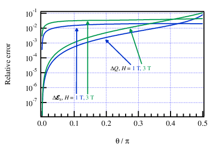
The result is markedly better than that obtained using perturbation theory (Fig. 6), even for greater values of the angle . This can be easily explained by the fact that the classical model is based on a much different approximation, namely that the spin only slightly deviates from being aligned with the easy () axis. This gives a validity over a much greater range than what was given by treating the transverse field as a perturbation.
IV Anisotropic properties of magnetic deflagration and detonation
IV.1 Magnetic deflagration
In this subsection, we investigate the magnetic deflagration speed for an arbitrary angle between the magnetic field and the easy axis; the next subsection will be devoted to magnetic detonation. We stress here that the propagation of magnetic deflagration involves four important vector values: the magnetic field intensity , the magnetization , the temperature gradient , and the heat flux (with being the tensor of thermal conduction). The latter two are in general not parallel because of the crystal anisotropy. Among these values, the temperature gradient determines the direction of front propagation, while the magnetic field intensity and magnetization specify the activation energy and the Zeeman energy of the spin reversal as discussed in the previous sections. We stress that the vectors and are not related to the direction of the deflagration front velocity, but influence the absolute value of that velocity. We also point out that 1) the direction of the magnetic field is controlled by the experimental set-up; 2) the direction of the magnetization correlates strongly with the easy axis (c-axis) of the crystal (see the calculations above and Fig. 2); 3) the direction of the temperature gradient and front propagation are determined by the ignition conditions, e.g., by surface acoustic waves;[18] and 4) the direction of the heat flux results from the anisotropic thermal conduction of the crystal. The different directions defined by these four vectors open a wide parameter space for experimental studies of anisotropic crystal properties, both magnetic and thermal. As an example, Fig. 8

illustrates some possibilities of the magnetic deflagration geometry [because of the small factor in the Hamiltonian for Mn12-acetate (see Tab. 1) the difference between the a and b crystal axes is minor]. Figure 8(a) shows the commonly investigated case of a deflagration front propagating along the easy axis with the magnetic field and magnetization aligned along the same axis. In Fig. 8(b), the magnetic field points along the easy axis, but the magnetic deflagration front propagates along the hard axis (axis a or b). Obviously, both the activation and Zeeman energies are the same for the geometries of Fig. 8(a) and (b); but the deflagration speed is different because of different thermal conduction along the easy and hard axes. In particular, by comparing the magnetic deflagration speed for these two geometries, and , one can measure the ratio of the thermal conduction coefficients quantitatively as . Finally, Fig. 8(c) shows the geometry with the front propagating along the easy axis, but with the magnetic field directed at some arbitrary angle to the axis. In this section we focus on the geometry of Fig. 8(c). For large magnetization values, , this geometry involves refraction of the magnetic field at the deflagration front. Still, for the crystals of nanomagnets used in the experimental studies so far, the magnetization is small, , and the refraction effects may be neglected. In principle, one may consider an even more general geometry than that shown in Fig. 8(c) with both the magnetic field and the front speed aligned at some angle to the easy axis. However, at present there is no quantitative experimental data for the ratio ; therefore, such a general case involves unidentified parameters and, without proper experimental support, it may be considered only as an hypothetical study. A qualitative comparison of the coefficients of thermal conduction along different axes was performed in Ref. 30 for crystals of , leading to the evaluation that . Assuming the same tendency for -acetate, one should expect that the thermal anisotropy somewhat moderates the strong effects of magnetic anisotropy obtained below. Still, a noticeable influence of thermal anisotropy is unlikely since the difference between the coefficients of thermal conduction is presumably only by a numerical factor of order of unity and the magnetic deflagration speed depends rather weakly on as . In contrast to that, we show below that magnetic anisotropy leads to variations of the magnetic deflagration speed by two orders of magnitude.
Within the geometry of Fig. 8(c), the governing equations for magnetic deflagration are[19, 20]
| (35) |
and
| (36) |
where is the phonon energy, is temperature, is the fraction of molecules in the metastable state (i.e., normalized concentration), is the coefficient of time dimension characterizing the kinetics of the spin switching. We also take into account here the possibility of a non-zero final fraction of molecules in the metastable state in the case of relatively low heating (low Zeeman energy), which has been termed “incomplete magnetic burning” in Ref. 19. This fraction is given by[19, 20]
| (37) |
which is (obviously) taken into account in Eq. (36); here the label refers to the final state of the system after the avalanche. As we can see from Figs. 9 and 10, the concentration cannot be neglected in the case of a small magnetic field and/or strong misalignment with the c-axis. The phonon energy and crystal temperature in Eqs. (35) and (36) are related according to[19, 35]
| (38) |
where corresponds to the simple crystal model, is the Boltzmann constant, is the problem dimension (we take , as we consider the 3D case), is the Debye temperature, with K for acetate. The thermal conduction may also depend on temperature; Refs. 19, 20 considered the dependence in the form with the parameter within the range 0 to 13/3. Below we show that the case of constant thermal conduction, i.e., , gives the best fit to the experimental data.[17]
We consider the stationary solution to Eqs. (35) and (36) for a planar magnetic deflagration front propagating with constant velocity along the -axis (the easy axis). In the reference frame of the front, Eqs. (35) and (36) reduce to
| (39) |
| (40) |
The boundary conditions for the system are determined by the initial energy (temperature ) far ahead of the front, and the final energy (temperature ) far behind the front. The initial and final energies (temperatures) are related by the condition of energy conservation , or
| (41) |
which follows from Eq. (39). In particular, our calculations use a low initial temperature, K, which allows reducing Eq. (41) to the simpler form
| (42) |
We calculate final temperature and the final molecule fraction in the metastable state numerically for different strengths and inclinations of the magnetic field; the results obtained are presented in Figs. 9 and 10 together with the scaled activation energy , which plays an important role for the deflagration front dynamics. As we can see, the temperature increases with the field and decreases with the angle; the scaled activation energy decreases with the field and increases with the angle. Still, this decrease/increase is not dramatic; for example, for , the temperature changes from to and the scaled activation energy from to as the angle varies from to . We will see below that the variations of the deflagration speed are much stronger because the speed is sensitive to both the final temperature and the scaled activation energy.


A qualitative understanding of the magnetic deflagration speed may be obtained from the Zeldovich-Frank-Kamenetsky theory, from which we have the expression[36, 19]
| (43) |
where is the Zeldovich number,
| (44) |
and is the heat capacity in the heated crystal. The final relation in Eq. (44) becomes an accurate equality for the case of complete magnetic burning, . The Zeldovich-Frank-Kamenetsky theory, giving the speed [Eq. (43)], holds only for large values of the Zeldovich number . Such large values are common in combustion problems,[23, 24] but rather unusual for magnetic deflagration. As we can see from Figs. 9 and 10, the Zeldovich-Frank-Kamenetsky theory may be applied to magnetic deflagration only for the cases of sufficiently low field and high angles between the magnetic field and the easy axis approaching . In the case of a moderate Zeldovich number, as often encountered in magnetic deflagration, the deflagration speed may be calculated numerically on the basis of Eqs. (39) and (40) using the numerical method of Refs. 20, 37.
We point out that the problem contains a number of parameters whose experimental measurement still remain a challenging task, such as the thermal conduction and the coefficient of time dimension characterizing spin-switching . The temperature dependence of thermal conduction is also unclear, with the factor treated as a free parameter in Refs. 19, 37 changing within the range of . We suggest here choosing particular values of the unknown parameters by comparing numerical results to the experimental data[17] obtained for the magnetic field aligned along the easy axis. Figure 11 presents the magnetic deflagration speed versus the magnetic field calculated for different values of and . Comparison to the experimental data suggests the parameter values and , which provide the best fit for the experimental results (red line) and which we use in the following for investigating the anisotropic properties of magnetic deflagration. The method of least squares was used to fit the data. As we can see in Fig. 11, a strong temperature dependence of the thermal conduction with leads to an excessively strong dependence of the deflagration speed on the magnetic field, which does not reproduce the experimental data properly. Figure 11 shows also the analytical predictions of the Zeldovich-Frank-Kamenetsky theory, Eq. (43), plotted by the dashed line for the same parameters and as the numerical solution. As we can see, the analytical theory provides only qualitative predictions in the experimentally interesting parameter range.


The numerical results for the magnetic deflagration speed are presented in Fig. 12: (a) versus the angle between the magnetic field and the easy axis for different strength of the magnetic field; (b) versus the magnetic field strength for different values of the angle. All plots in Fig. 12 demonstrate the same tendencies – monotonic increase of the deflagration speed with the field and strong decrease with the angle. The tendencies are qualitatively the same as one had for the final temperature; still, they are much more dramatic for the deflagration speed. In particular, for a field strength of we find the deflagration speed for for the magnetic field aligned along the easy axis (), a much smaller speed for and a negligible value for the magnetic field perpendicular to the easy axis with . Thus we obtain a magnetic deflagration speed almost two orders of magnitude smaller for the magnetic field directed along the hard axis in comparison with that directed along the easy axis. Here we stress that the difference in the deflagration speed in our study comes only from modifications in the activation energy and Zeeman energy while the thermal conduction coefficient remains the same. This is different from the experimental studies of Ref. 30 for where the deflagration speed changes both because of misalignment of the magnetic field and thermal conduction simultaneously. As a result, the geometry suggested here provides better conditions for investigating quantum-mechanical properties of the nanomagnets (i.e., magnetic anisotropy) and thermal properties of the crystals separately. We also stress that the present numerical results rely on the available models for the nanomagnet Hamiltonian for Mn12-acetate;[16] by modifying the coefficients in the Hamiltonian one comes to other numerical values for the magnetic deflagration speed. The present work may also serve for solving the inverse problem: by comparing the numerical predictions to future refined experiments one may adjust the coefficients in the Hamiltonian for nanomagnets.
IV.2 Magnetic detonation

The same method may also be used to investigate anisotropic properties of magnetic detonation. In contrast to deflagration, magnetic detonation propagates due to a leading shock wave preheating the initially cold crystal, see Fig. 13 for typical profiles of temperature, pressure and fraction of molecules in the metastable state. For comparison, in magnetic deflagration, preheating happens due to thermal conduction, which is negligible for the fast process of magnetic detonation. Another important feature of Fig. 13 (a) is that the preheating zone for magnetic deflagration is comparable by width to the zone of spin switching and energy release at . This is qualitatively different from the analytical Zeldovich-Frank-Kamenetsky deflagration model,[19, 36] which assumes a wide preheating region and an extremely narrow zone of energy release. We also point out that magnetic detonation is noticeably different from the common detonation model (the Zeldovich-von Neumann-Doring model) employed in combustion science. In particular, the combustion model involves a strong delay of the energy release behind the leading shock.[23] In contrast to that, in magnetic detonation the spin switching and energy release start directly at the leading shock at . The most important properties of magnetic detonation propagating along the easy axis have been studied in Ref. 22. In particular, Ref. 22 has demonstrated that magnetic detonation is ultimately weak in comparison with common combustion detonations[23] and, therefore, it propagates with a velocity only slightly exceeding the sound speed ( for Mn12-acetate). As a result, the magnetic detonation speed does not depend on the direction of the magnetic field. Unlike that, other properties of magnetic detonation are quite sensitive to the energy release in the spin switching and hence to the magnetic field direction. This dependence concerns first of all the temperature behind the leading shock (label s), which may be calculated as[22]

| (45) |
where is the Gruneisen coefficient, and the factor characterizes the elastic contribution to the pressure , where is the initial density of the crystal, see Ref. 22 for details. The temperature behind the magnetic detonation front (labeled d) depends also on the Zeeman energy release as
| (46) |
The characteristic times of spin switching in magnetic detonation at the shock, , and at the final detonation temperature, , are also strongly influenced by the direction of the magnetic field. The anisotropic dependence of the temperature on the angle between the magnetic field and the easy axis is presented in Fig. 14.

Similarly to deflagration, the temperature in magnetic detonation exhibits noticeable, though not dramatic, decrease with the angle between the magnetic field and the easy axis. For example, for , the temperature just behind the shock changes from at to at ; the resulting temperature behind the magnetic detonation front changes from at to at . However, these moderate modifications of temperature, together with respective modifications of the activation energy, lead to dramatic changes in the characteristic spin-switching time at the shock, , and at the final detonation temperature, , as shown in Fig. 15. For example, for the same magnetic field strength as used in the above example, , we find the reversal time behind the leading shock at and at ; thus we observe variations of the reversal time by six orders of magnitude. Such an increase of the spin-reversal time makes the magnetic detonation front unrealistically wide at large angles so that magnetic detonation becomes impossible for noticeable misalignment between the external magnetic field and the easy axis. The characteristic spin-switching time at the final temperature and the external field changes from at to at . Note that in Fig. 14 we consider larger values of the external magnetic field than those used in the magnetic deflagration experiments. As pointed out in Ref. 22, moderate magnetic fields lead to a quite large thickness of the magnetic detonation front, , much larger than the typical sample size unless the magnetic detonation is formed at a specific resonant field characterizing nanomagnets.[21] Investigation of spin avalanches at the resonant field requires further work beyond the scope of the present paper.
V Summary
In this paper, we have investigated anisotropic properties of spin avalanches in crystals of nanomagnets propagating in the form of pseudo-combustion fronts – magnetic deflagration and detonation. In general, the anisotropy is expected to be of two types: magnetic and thermal. We have focused here on the magnetic anisotropy related to the misalignment of the external magnetic field and the easy axis of the crystal. The thermal anisotropy is not considered since at present there is no sufficient experimental data for such a study.
The magnetic anisotropy affects primarily two values of the key importance for the magnetic deflagration and detonation dynamics – the activation energy and the Zeeman energy. Here, we calculated the activation and Zeeman energies as a solution to the quantum-mechanical problem of a single nanomagnet of -acetate placed in the external magnetic field, which is then reversed. We demonstrated strong dependence of the activation and Zeeman energies on the strength and direction of the external magnetic field.
We obtained that, because of this strong dependence, the magnetic deflagration speed is quite sensitive to the direction of the magnetic field too. In particular, we found that the magnetic deflagration speed may decrease by two orders of magnitude for the magnetic field aligned along the hard crystal axis instead of the easy one.
In contrast to magnetic deflagration, the magnetic detonation speed is determined mostly by the sound speed in the crystal and, hence, does not depend on the direction of the magnetic field. At the same time, other properties of magnetic detonation, such as the temperature behind the leading shock and for completed spin reversal, and the characteristic time of spin switching, demonstrate a strong anisotropy.
Acknowledgements.
Financial support from the Swedish Research Council and the Faculty of Natural Sciences, Umeå University is gratefully acknowledged. The authors thank Myriam Sarachik for useful discussions.References
- [1] T. Lis, Acta Crystallogr. Sect. B 36, 2042 (1980).
- [2] A. Caneschi, D. Gatteschi, R. Sessoli, A. L. Barra, L. C. Brunel, and M. Guillot, J. Am. Chem. Soc. 113, 5873 (1991).
- [3] G. C. Papaefthymiou, Phys. Rev. B 46, 10366 (1992).
- [4] R. Sessoli, H. L. Tsai, A. R. Schake, S. Wang, J. B. Vincent, K. Folting, D. Gatteschi, G. Christou, and D. N. Hendrickson, J. Am. Chem. Soc. 115, 1804 (1993a).
- [5] For example, -acetate has a core of four () surrounded by a ring of eight (), producing a ferromagnetic structure with a total spin number , see, e.g., Ref. \rev@citealpnummag:thomas96.
- [6] R. Sessoli, D. Gatteschi, A. Caneschi, and M. A. Novak, Nature 365, 141 (1993b).
- [7] J. Villain, F. Hartman-Boutron, R. Sessoli, and A. Rettori, Europhys. Lett. 27, 159 (1994).
- [8] C. Paulsen, J.-G. Park, B. Barbara, R. Sessoli, and A. Caneschi, J. Magn. Magn. Mater. 140–144, 379 (1995).
- [9] J. R. Friedman, M. P. Sarachik, J. Tejada, and R. Ziolo, Phys. Rev. Lett. 76, 3830 (1996).
- [10] L. Thomas, F. Lionti, R. Ballou, D. Gatteschi, R. Sessoli, and B. Barbara, Nature 383, 145 (1996).
- [11] D. A. Garanin and E. M. Chudnovsky, Phys. Rev. B 56, 11102 (1997).
- [12] E. M. Chudnovsky and J. Tejada, Macroscopic Quantum Tunneling of the Magnetic Moment (Cambridge University Press, Cambridge, 1998).
- [13] J. Villain and A. Fort, Eur. Phys. J. B 17, 69 (2000).
- [14] W. Wernsdorfer, Adv. Chem. Phys. 118, 99 (2001).
- [15] D. Gatteschi and R. Sessoli, Angew. Chem. Int. Ed. 42, 268 (2003).
- [16] E. del Barco, A. D. Kent, S. Hill, J. M. North, N. S. Dalal, E. M. Rumberger, D. N. Hendrickson, N. Chakov, and G. Christou, J. Low Temp. Phys. 140, 119 (2005).
- [17] Y. Suzuki, M. P. Sarachik, E. M. Chudnovsky, S. McHugh, R. Gonzalez-Rubio, N. Avraham, Y. Myasoedov, E. Zeldov, H. Shtrikman, N. E. Chakov, and G. Christou, Phys. Rev. Lett. 95, 147201 (2005).
- [18] A. Hernández-Mínguez, J. M. Hernandez, F. Macià, A. García-Santiago, J. Tejada, and P. V. Santos, Phys. Rev. Lett. 95, 217205 (2005).
- [19] D. A. Garanin and E. M. Chudnovsky, Phys. Rev. B 76, 054410 (2007).
- [20] M. Modestov, V. Bychkov, and M. Marklund, Phys. Rev. B 83, 214417 (2011a).
- [21] W. Decelle, J. Vanacken, V. V. Moshchalkov, J. Tejada, J. M. Hernández, and F. Macià, Phys. Rev. Lett. 102, 027203 (2009).
- [22] M. Modestov, V. Bychkov, and M. Marklund, Phys. Rev. Lett. 107, 207208 (2011b).
- [23] C. K. Law, Combustion Physics (Cambridge University Press, Cambridge, 2006).
- [24] V. Bychkov and M. Liberman, Phys. Rep. 325, 115 (2000).
- [25] V. Bychkov, A. Petchenko, V. Akkerman, and L.-E. Eriksson, Phys. Rev. E 72, 046307 (2005).
- [26] V. Bychkov, D. Valiev, and L.-E. Eriksson, Phys. Rev. Lett. 101, 164501 (2008).
- [27] S. B. Dorofeev, Proc. Combust. Inst. 33, 2161 (2011).
- [28] M. P. Sarachik (private communication); Y. Suzuki, Ph. D. Thesis, City University of New York, 2007.
- [29] F. Macià, J. M. Hernandez, J. Tejada, S. Datta, S. Hill, C. Lampropoulos, and G. Christou, Phys. Rev. B 79, 092403 (2009).
- [30] S. Vélez, J. M. Hernandez, A. García-Santiago, J. Tejada, V. K. Pecharsky, K. A. Gschneidner, D. L. Schlagel, T. A. Lograsso, and P. V. Santos, Phys. Rev. B 85, 054432 (2012).
- [31] V. Bychkov, P. Matyba, V. Akkerman, M. Modestov, D. Valiev, G. Brodin, C. K. Law, M. Marklund, and L. Edman, Phys. Rev. Lett. 107, 016103 (2011).
- [32] M. Modestov, V. Bychkov, D. Valiev, and M. Marklund, J. Phys. Chem. C 115, 21915 (2011c), http://pubs.acs.org/doi/pdf/10.1021/jp205415y .
- [33] V. Bychkov, O. Jukimenko, M. Modestov, and M. Marklund, Phys. Rev. B 85, 245212 (2012).
- [34] N. G. Koloskova, Fiz. Tverd. Tela 5, 61 (1963), [English transl.: Soviet Phys. – Solid State 5, 40 (1963)].
- [35] C. Kittel, Quantum Theory of Solids (Wiley, New York, 1963).
- [36] Y. Zeldovich, G. Barenblatt, V. Librovich, and G. Makhviladze, Mathematical Theory of Combustion and Explosions (Consultants Bureau, New York, 1985).
- [37] M. Modestov, V. Bychkov, D. Valiev, and M. Marklund, Phys. Rev. E 80, 046403 (2009).