A computer-assisted uniqueness proof for a semilinear elliptic boundary value problem
Abstract.
A wide variety of articles, starting with the famous paper [11], is devoted to the uniqueness question for the semilinear elliptic boundary value problem in , in , on , where ranges between and the first Dirichlet Laplacian eigenvalue. So far, this question was settled in the case of being a ball and, for more general domains, in the case . In [16], we proposed a computer-assisted approach to this uniqueness question, which indeed provided a proof in the case , and . Due to the high numerical complexity, we were not able in [16] to treat higher values of . Here, by a significant reduction of the complexity, we will prove uniqueness for the case .
Key words and phrases:
semilinear elliptic boundary value problem, uniqueness, computer-assisted proof2010 Mathematics Subject Classification
35J25, 35J60, 65N15Dedicated to the memory of Wolfgang Walter
1. Introduction
The semilinear elliptic boundary value problem
| (1.1) |
has attracted a lot of attention since the 19th century. Questions of existence and multiplicity have been (are still being) extensively studied by means of variational methods, fixed-point methods, sub- and supersolutions, index and degree theory, and more.
In this article, we will address the question of uniqueness of solutions for the more special problem
where ranges between and , the first eigenvalue of the Dirichlet Laplacian. It has been shown in a series of papers [19], [29], [28], [1], [2] that the solution of (1) is indeed unique when is a ball, or when is more general but ([30], [12], [9], [10]).
We will concentrate on the case where and , and prove that uniqueness holds for the full range of . Thus, our paper constitutes the first uniqueness result for this situation. More precisely we prove
Theorem 1.1.
Let be the unit square in , . Then the problem
admits only one solution for any .
Remark 1.1. a) A simple scaling argument shows that our uniqueness result carries over to all squares (and thus, to all squares in ): If is a positive solution of in , on , for some , then is a solution of (1.1) for .
b) Since we also show that the unique solution in the square is nondegenerate, by a result of [10] we deduce that the solution is unique also in domains “close to” a square.
c) Finally we observe that having shown in [16] (case ) and in this paper (case ) that the unique solution is nondegenerate then uniqueness follows also for other nonlinearities of the type for close to and . Indeed, by standard arguments (see for example [9]) nonuniqueness of positive solutions in correspondence to sequences of exponents converging to (resp. to ) would imply degeneracy of the solution for (resp. ).
Our proof heavily relies on computer-assistance. Such computer-assisted proofs are receiving an increasing attention in the recent years since such methods provided results which apparently could not be obtained by purely analytical means (see [6], [5], [24], [17], [18]).
We compute a branch of approximate solutions and prove existence of a true solution branch close to it, using fixed point techniques. By eigenvalue enclosure methods, and an additional analytical argument for close to we deduce the non-degeneracy of all solutions along this branch, whence uniqueness follows from the known bifurcation structure of the problem.
In [16] we give a general description of these computer-assisted means and use them to
obtain the
desired uniqueness result for the case . To make the present paper dealing
with the case more self-contained, we recall parts of the content of [16] here.
We remark
that the numerical tools used in [16] turned out not to be sufficient to treat the
case .
Now, by some new trick to reduce the numerical complexity, we are able to handle this case.
2. Preliminaries
In the following, let . We remark that the results of this section can be carried over to the more general case of a “doubly symmetric” domain; see [16] for details.
First, note that problem (1) can equivalently be reformulated as finding a non-trivial solution of
since, for , by the strong maximum principle (for ) every non-trivial solution of (2) is positive in . In fact, this formulation is better suited for our computer-assisted approach than (1).
As a consequence of the classical bifurcation theorem of [25] and of the results of [9] the following result was obtained in [20]:
Theorem 2.1.
We recall that the uniqueness of the solution of (1) for was proved in [10] and [9]. As a consequence of the previous theorem we have
Corollary 2.1.
If all solutions on the curve are nondegenerate then problem (1) admits only one solution for every .
Proof. The nondegeneracy of the solutions implies, by the Implicit Function Theorem, that
neither turning points nor secondary bifurcations can exist along . Then, for every there exists only one solution of (1) on . By
Theorem 2.1 all solutions are on , hence uniqueness follows. ∎
Theorem 2.1 and Corollary 2.1 indicate that to prove the uniqueness of the
solution of problem (1) for every it is enough to
construct a branch of nondegenerate solutions which connects to .
This is what we will do numerically in the next sections with a rigorous computer-assisted proof.
However, establishing the nondegeneracy of solutions for close to numerically can be difficult, due to the fact that the only solution at , which is the identically zero solution, is obviously degenerate because its
linearized operator is which has the first eigenvalue equal to zero.
The next proposition shows that there exists a
computable number such that for any problem (1) has only one solution which
is also nondegenerate. Of course, from the well-known results of Crandall and Rabinowitz,
[7, 8], one can establish that for “close to” , all solutions are nondegenerate. However, in order to complete our program, we need to calculate a
precise and explicit estimate of how close they need to be. This allows us to carry out the
numerical computation only in the interval as we will do later.
Let us denote by and the first and second eigenvalue of the operator in with homogeneous Dirichlet boundary conditions. We have
Proposition 2.1.
(Recall that is the unique continuous branch of solutions given by Theorem 2.1.)
Proof. see [16]
Corollary 2.2.
Proof. We set with connecting to
. On
we have that all solutions are nondegenerate by i). On the other hand the hypothesis ii)
allows us to apply Proposition 2.1
which shows nondegeneracy of all solutions on .
Hence there is nondegeneracy all along so
the assertion follows from Corollary 2.1. ∎
The last corollary suggests the method of proving the uniqueness through computer assistance: first we construct a branch of nondegenerate “true” solutions near approximate ones in a certain interval and then verify ii) for the solution . Note that the estimate (2.6) depends only on and on the eigenvalues and of the operator in the domain . So the constant on the right-hand side is easily computable. When is the unit square which is the case analyzed in the next sections, the estimate (2.6) becomes:
because and .
Fixing we finally get the condition
| (2.7) |
3. The basic existence and enclosure theorem
We start the computer-assisted part of our proof with a basic theorem on existence, local uniqueness, and non-degeneracy of solutions to problem (2), assuming now for simplicity of presentation. In this section, the parameter is fixed.
Let be endowed with the inner product ; actually we choose in this paper, but different (usually positive) choices of are advantageous or even mandatory in other applications, whence we keep as a parameter in the following. Let denote the (topological) dual of , endowed with the usual operator .
Suppose that an approximate solution of problem (2) has been computed by numerical means, and that a bound for its defect is known, i.e.
| (3.1) |
as well as a constant such that
| (3.2) |
Here, denotes the operator linearizing problem (2) at ; more generally, for , let the linear operator be defined by
| (3.3) |
The practical computation of bounds and will be addressed in Sections 6, 7 and 8.
Let denote a norm bound (embedding constant) for the embedding , which is bounded since . can be calculated e.g. according to the explicit formula given in [23, Lemma 2]. Finally, let
In our example case where , the above-mentioned explicit formula gives (with the choice )
Theorem 3.1.
Suppose that some exists such that
| (3.4) |
and
| (3.5) |
For a proof, see [16].
Corollary 3.1.
Remark 3.1. a) The function has obviously a positive maximum at , and the crucial condition (3.4) requires that
| (3.13) |
i.e. has to be sufficiently small. According to (3.1), this means that must be computed with sufficient accuracy, which leaves the “hard work” to the computer!
Furthermore, a “small” defect bound allows (via (3.4)) a “small” error bound , if is not too large.
4. The branch
Fixing some (the actual choice of which is made on the basis of Proposition 2.1; see also Section 5), we assume now that for every an approximate solution is at hand, as well as a defect bound satisfying (3.1), and a bound satisfying (3.2). Furthermore, we assume now that, for every , some satisfies (3.4) and (3.5), and the additional non-triviality condition (see Corollary 3.1). We suppose that some uniform (-independent) can be chosen such that (3.5) holds with instead of (compare Theorem 3.1 b)). Hence Theorem 3.1 gives a positive solution of problem (2) with the properties (3.6), (b)), (c)), for every .
Finally, we assume that the approximate solution branch , is continuous, and that is lower semi-continuous.
In Sections 6, 7 and 8, we will address the actual computation of such branches .
So far we know nothing about continuity or smoothness of , which however we will need to conclude that coincides with the sub-branch introduced in Corollary 2.2.
Theorem 4.1.
The solution branch
is continuously differentiable.
Proof: The mapping
is continuously differentiable, with (see (3.3)), and for all . Using the Mean Value Theorem one can show that depends indeed continuously on ; see [16, Lemma 3.1] for details.
It suffices to prove the asserted smoothness locally. Thus, fix . Since is bijective by Theorem 3.1 c), the Implicit Function Theorem gives a -smooth solution branch
to problem (2), with . By (3.6),
| (4.4) |
Since and depend continuously on , and lower semi-continuously, (4.4) implies
for some . Hence Theorem 3.1 b) provides
implying the desired smoothness in some neighborhood of (which of course is one-sided if or . ∎
As a consequence of Theorem 4.1, is a continuous solution curve connecting the point with , and thus must coincide with the sub-branch , connecting these two points, of the unique simple continuous curve given by Theorem 2.1. Using Theorem 3.1 c), we obtain
Corollary 4.1.
On the sub-branch of which connects with , all solutions are nondegenerate.
5. Choice of
We have to choose such that condition (2.6) is satisfied. For this purpose, we use computer-assistance again. With denoting the intersection of the symmetry axes of the (doubly symmetric) domain , i.e. for , we choose , not too close to , such that our approximate solution satisfies
| (5.1) |
with “not too small” difference between right- and left-hand side. Such a can be found within a few numerical trials.
Here, we impose the additional requirement
| (5.2) |
which is in fact a condition on the numerical method used to compute . (Actually, condition (5.2) could be avoided if we were willing to accept additional technical effort.) Moreover, exceeding (3.1), we will now need an -bound for the defect:
| (5.3) |
Finally, we note that is convex, and hence in particular -regular, whence every solution of problem (2) is in .
Using the method described in Section 3, we obtain, by Theorem 3.1 a), a positive solution of problem (2) satisfying
| (5.4) |
Now we make use of the explicit version of the Sobolev embedding given in [21]. There, explicit constants , , are computed such that
with denoting the -Frobenius norm of the Hessian matrix . E.g. for , [21] gives
Moreover, for since is convex (see e.g. [14]). Consequently,
| (5.5) |
To bound the last term on the right-hand side, we first note that
| (5.6) | |||||
| (5.7) |
using (5.4) and an embedding constant for the embedding in the last but one line; see e.g. [23, Lemma 2] for its computation. Moreover, by (2) and (5.3),
| (5.8) |
Using (5.4) - (5.8), and the Poincaré inequality
| (5.9) |
we finally obtain
| (5.10) |
and the right-hand side is “small” if and are “small”, which can (again) be achieved by sufficiently accurate numerical computations.
Finally, since
(5.10) yields an upper bound for which is “not too much” larger than . Hence, since by [11], condition (2.6) can easily be checked, and (5.1) (with “not too small” difference between right- and left-hand side) implies a good chance that this check will be successful; otherwise, has to be chosen a bit larger.
6. Computation of and for fixed
In this section we report on the computation of an approximate solution to problem (2), and of bounds and satisfying (3.1) and (3.2), where is fixed (or one of finitely many values). We will again restrict ourselves to the unit square .
An approximation is computed by a Newton iteration applied to problem (2), where the linear boundary value problems
| (6.1) |
occurring in the single iteration steps are solved approximately by an ansatz
| (6.2) |
and a Ritz-Galerkin method (with the basis functions in (6.2)) applied to problem (6.1). The update concludes the iteration step.
The Newton iteration is terminated when the coefficients in (6.2) are “small enough”, i.e. their modulus is below some pre-assigned tolerance.
To start the Newton iteration, i.e. to find an appropriate of the form (6.2), we first consider some close to , and choose ; with an appropriate choice of (to be determined in a few numerical trials), the Newton iteration will “converge” to a non-trivial approximation . Then, starting at this value, we diminish in small steps until we arrive at , while in each of these steps the approximation computed in the previous step is taken as a start of the Newton iteration. In this way, we find approximations to problem (2) for “many” values of . Note that all approximations obtained in this way are of the form (6.2).
The computation of an -defect bound satisfying
| (6.3) |
amounts to the computation of an integral over .
Due to [11] every solution of (2) is symmetric with respect to reflection at the axes and . Therefore it is useful to look for approximate solutions of the form
| (6.4) |
Using sum formulas for and one obtains for all
and thus can be written as follows:
| (6.5) |
Since ranges in and is positive for , will be positive if
| (6.6) |
Condition (6.6) can easily be checked using interval arithmetic and is indeed always satisfied for our approximate solutions, since turns out to be “dominant” and the higher coefficients decay quickly. Hence is positive and one can omit the modulus in the computations. Therefore the integral in (6.3) can be computed in closed form, since only products of trigonometric functions occur in the integrand. After calculating them, various sums remain to be evaluated. In order to obtain a rigorous bound , these computations (in contrast to those for obtaining as described above) need to be carried out in interval arithmetic [13, 27], to take rounding errors into account.
Note that the complexity in the evaluation of the defect integral in (6.3), without any further modifications, is due to the term . Using some trick, it is however possible to reduce the complexity to :
Applying the sum formulas and one obtains:
Since , we get
Setting for the previous sum can be rewritten as
For fixed and each of the two double-sums in parentheses is .
Since they are independent, the product is still . The sums over and then give
, whereas the sums over and do not change the complexity.
Moreover the sum is only
Similarly, also certain constellations of reduce the -sum, and of course analogous reductions are possible for the -sum. Since if or is even, the result does not change if the sum is only taken over odd values of and .
Remark 6.1. a) Computing trigonometric sums in an efficient way is an object of investigation since a very long time, but up to our knowledge the above complexity reduction has not been published before.
b) As an alternative to the closed form integration described above, we also tried quadrature for computing the defect integral, but due to the necessity of computing a safe remainder term bound in this case, we ended up in a very high numerical effort, since a large number of quadrature points had to be chosen. So practically closed-form integration turned out to be more efficient, although its complexity (as ) is higher than the quadrature complexity.
Once an -defect bound (satisfying (6.3)) has been computed, an -defect bound (satisfying (3.1)) is easily obtained via the embedding
| (6.7) |
which is a result of the corresponding dual embedding (5.9). Indeed, (6.3) and (6.7) imply that
satisfies (3.1).
The estimate (6.7) is suboptimal but, under practical aspects, seems to be the most suitable way for obtaining an -bound for the defect. At this point we also wish to remark that, as an alternative to the weak solutions approach used in this paper, we could also have aimed at a computer-assisted proof for strong solutions (see [23]), leading to -and -error bounds; in this case an -bound is needed directly (rather than an -bound).
7. Computation of for fixed
For computing a constant satisfying (3.2), we use the isometric isomorphism
and note that is -symmetric since
| (7.4) |
and hence selfadjoint. Since , (3.2) thus holds for any
| (7.5) |
provided the min is positive.
A particular consequence of (7.4) is that
| (7.6) |
where
| (7.7) |
Note that, due to the positivity of our approximate solutions established in
Section 6, the modulus can be omitted here, which again facilitates numerical computations.
Choosing a positive parameter in the -product (recall that we actually chose
), we obtain on .
Thus, (7.6) shows that all eigenvalues of
are less than , and that its essential spectrum consists of the single point . Therefore,
(7.5) requires the computation of eigenvalue bounds for the eigenvalue(s)
neighboring .
Using the transformation , the eigenvalue problem is easily seen to be equivalent to
or, in weak formulation,
| (7.8) |
and we are interested in bounds to the eigenvalue(s) neighboring . It is therefore sufficient to compute two-sided bounds to the first eigenvalues of problem (7.8), where is (at least) such that . In all our practical examples, the computed enclosures are such that , whence by (7.5) and we can choose
| (7.9) |
Remark 7.1. By [11] and the fact that is symmetric with respect to reflection at the axes and , all occurring function spaces can be replaced by their intersection with the class of reflection symmetric functions. This has the advantage that some eigenvalues drop out, which possibly reduces the constant .
The desired eigenvalue bounds for problem (7.8) can be obtained by computer-assisted
means of their own. For example, upper bounds to (with
given) are easily and efficiently computed by the Rayleigh-Ritz method [26]:
Let denote linearly independent
trial functions, for example approximate eigenfunctions obtained by numerical means, and form the
matrices
Then, with denoting the eigenvalues of the matrix eigenvalue problem
(which can be enclosed by means of verifying numerical linear algebra; see [3]), the Rayleigh-Ritz method gives
However, also lower eigenvalue bounds are needed, which constitute a more complicated task
than upper bounds. The most accurate method for this purpose has been proposed by Lehmann
[15], and improved by Goerisch concerning its range of applicability [4]. Its
numerical core is again (as in the Rayleigh-Ritz method) a matrix eigenvalue problem, but the
accompanying analysis is more involved. In particular, in order to compute lower bounds to the first
eigenvalues, a rough lower bound to the -st eigenvalue must be known already. This
a priori information can usually be obtained via a homotopy method connecting a simple “base
problem” with known eigenvalues to the given eigenvalue problem, such that all eigenvalues increase
(index-wise) along the homotopy; see [22] or [5] for details on
this method, a detailed description of which would be beyond the scope of this article. In fact,
[5] contains the newest version of the homotopy method, where only very
small ( or even ) matrix eigenvalue problems need to be treated rigorously
in the course of the homotopy.
Finding a base problem for problem (7.8), and a suitable homotopy connecting them, is rather
simple here since is a bounded rectangle, whence the eigenvalues of on are known: We choose a constant upper bound for on , and the coefficient homotopy
Then, the family of eigenvalue problems
connects the explicitly solvable constant-coefficient base problem to problem (7.8)
, and the eigenvalues increase in , since the Rayleigh quotient does, by Poincaré’s
min-max principle.
8. Computation of branches
In the previous section we described how to compute approximations for a grid of finitely many values of within . After selecting (among these) according to Section 5, we are left with a grid
and approximate solutions . Furthermore, according to the methods described in the previous sections, we can compute bounds and such that (3.1) and (3.2) hold at .
Now we define a piecewise linear (and hence continuous) approximate solution branch by
| (8.1) |
To compute corresponding defect bounds , we fix and , and let , whence
| (8.2) |
Using the classical linear interpolation error bound we obtain, for fixed ,
| (8.3) |
| (8.4) |
Since for all , with denoting an embedding constant for the embedding (e. g. ), (8.3) and (8.4) imply
| (8.5) |
| (8.6) |
| (8.7) |
Thus, we obtain a branch of defect bounds
which is constant on each subinterval . In the points is possibly doubly defined by (8.7), in which case we
choose the smaller of the two values. Hence, is lower semi-continuous.
Note that given by (8.7) is “small” if and
are small (i.e. if the approximations and have been computed with
sufficient accuracy; see Remark 3.1a)) and if are small (i.e. if the grid is
chosen sufficiently fine; see (8.5), (8.6)).
| (8.8) |
whence a coefficient perturbation result given in [16, Lemma 3.2] implies: If
| (8.9) |
then (3.2) holds for
| (8.10) |
Note that (8.9) is indeed satisfied if the grid is chosen sufficiently fine, since then
and are “small” by (8.8).
Analogous estimates give also on the two remaining half-intervals and .
Choosing again the smaller of the two values at the points where is possibly doubly defined by (8.10), we
obtain a lower semi-continuous, piecewise constant branch .
According to the above construction, both and are constant on the half-intervals. Moreover, (8.1) implies that, for ,
and again we choose the smaller of the two values at the points of double definition.
Using these bounds, the crucial inequalities (3.4) and (3.5) (which have to be satisfied for all ) result in finitely many inequalities which can be fulfilled with “small” and piecewise constant if is sufficiently small, i.e. if have been computed with sufficient accuracy (see Remark 3.1a)) and if the grid has been chosen sufficiently fine (see (8.5) - (8.7)). Moreover, since , and the above piecewise constant upper bound for are lower semi-continuous, the structure of the inequalities (3.4) and (3.5) clearly shows that also can be chosen to be lower semi-continuous, as required in Section 4. Finally, since (3.5) now consists in fact of finitely many strict inequalities, a uniform (-independent) can be chosen in Theorem 3.1b), as needed for Theorem 4.1.
9. Numerical results
All computations have been performed on an AMD Athlon Dual Core 4800+ (2.4GHz) processor, using MATLAB (version R2010a) and the interval toolbox INTLAB [27]. For some of the time consuming nested sums occurring in the computations, we used moreover mexfunctions to outsource these calculations to C++. For these parts of the program we used C-XSC [13] to verify the results. Our source code can be found on our webpage11 1 http://www.math.kit.edu/iana2/~roth/page/publ/en.
In the following, we report on some more detailed numerical results.
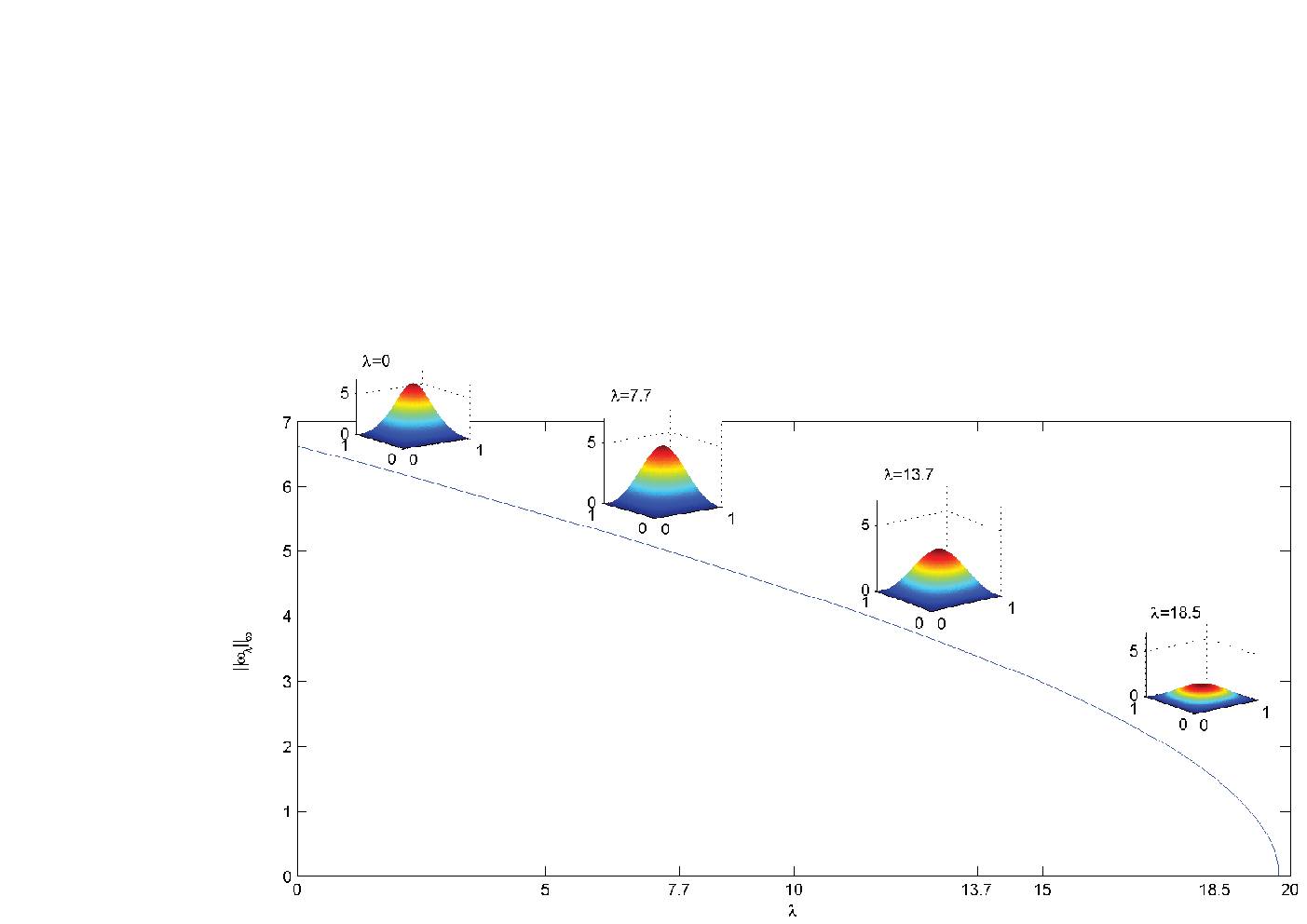
Using (which is not the minimally possible choice; e.g. could have been chosen) and values (with and the remaining gridpoints equally spaced with distance 0.2) we computed approximations with in (6.2), as well as defect bounds and constants , by the methods described in Section 6 and 7.
Figure 1 shows an approximate branch . The continuous plot has been created by interpolation of the above grid points , plus some more grid points between and , where we computed additional approximations.
For some selected values of , Table 1 shows, with an obvious sub- and superscript notation for enclosing intervals, the computed eigenvalue bounds for problem (7.8) (giving by (7.9)). These were obtained using the Rayleigh-Ritz and the Lehmann-Goerisch method, and the homotopy method briefly mentioned at the end of Section 7 (exploiting also the symmetry considerations addressed in Remark 7.1). The integer , needed for these procedures, has been chosen different (between and ) for different values of , according to the outcome of the homotopy. This resulted in a slightly different quality of the eigenvalue enclosures.
Table 2 contains, for some selected of the 186 -half-intervals,
- a)
- b)
- c)
Thus, Corolllary 2.1, together with all the considerations in the previous sections, proves Theorem 1.1.
| -interval | |||
|---|---|---|---|
| [0,0.05) | 0.0005943 | 1.7443526 | 0.0010378 |
| (2,2.1) | 0.0023344 | 1.7707941 | 0.0041521 |
| (6,6.1) | 0.0022937 | 1.6669879 | 0.0038369 |
| (10,10.1) | 0.0023644 | 1.5677657 | 0.0037168 |
| (14,14.1) | 0.0026980 | 1.9582604 | 0.0053028 |
| (16,16.1) | 0.0031531 | 3.2267762 | 0.0102701 |
| (18.4,18.5] | 0.0050056 | 13.8930543 | 0.0882899 |
Acknowledgments. The authors are grateful to two anonymous referees for their helpful remarks and suggestions.
References
- [1] Adimurthi and S. Yadava, An elementary proof for the uniqueness of positive radial solution of a quasilinear Dirichlet problem, Arch. Rat. Mech. Anal., 126 (1994), pp. 219–229.
- [2] A. Aftalion and F. Pacella, Uniqueness and nondegeneracy for some nonlinear elliptic problems in a ball, Journ. Diff. Eq., 195 (2003), pp. 380–397.
- [3] H. Behnke, Inclusion of eigenvalues of general eigenvalue problems for matrices, in: U. Kulisch, H. J. Stetter (Eds.), Scientific Computation with Automatic Result Verification, Computing 6 (Suppl.) (1987), pp. 69–78.
- [4] H. Behnke and F. Goerisch, Inclusions for eigenvalues of selfadjoint problems, in: J. Herzberger (Ed.), Topics in Validated Computations, Series Studies in Computational Mathematics, North-Holland, Amsterdam (1994), pp. 277–322.
- [5] B. Breuer, J. Horak, P. J. McKenna, and M. Plum, A computer-assisted existence and multiplicity proof for travelling waves in a nonlinearly supported beam, J. Differential Equations, 224 (2006), pp. 60–97.
- [6] B. Breuer, P. J. McKenna, and M. Plum, Multiple solutions for a semilinear boundary value problem: a computational multiplicity proof, J. Differential Equations, 195 (2003), pp. 243–269.
- [7] M. G. Crandall and P. H. Rabinowitz, Bifurcation from simple eigenvalues, J. Functional Analysis, 8 (1971), pp. 321–340.
- [8] , Bifurcation, perturbation of simple eigenvalues and linearized stability, Arch. Rational Mech. Anal., 52 (1973), pp. 161–180.
- [9] L. Damascelli, M. Grossi, and F. Pacella, Qualitative properties of positive solutions of semilinear elliptic equations in symmetric domains via the maximum principle, Ann. Inst. H. Poincaré, 16 (1999), pp. 631–652.
- [10] E. N. Dancer, The effect of the domain shape on the number of positive solutions of certain nonlinear equations, Journ. Diff. Eq., 74 (1988), pp. 120–156.
- [11] B. Gidas, W. M. Ni, and L. Nirenberg, Symmetry and related properties via the maximum principle, Comm. Math. Phys., 68 (1979), pp. 209–243.
- [12] M. Grossi, A uniqueness result for a semilinear elliptic equation in symmetric domains, Adv. Diff. Equations, 5 (2000), pp. 193–212.
- [13] R. Klatte, U. Kulisch, C. Lawo, M. Rausch, and A. Wiethoff, C-XSC-A C++ Class Library for Extended Scientific Computing, Springer, Berlin, 1993.
- [14] O. A. Ladyzhenskaya and N. N. Ural’tseva, Linear and quasilinear elliptic equations, Academic Press, New York-London, 1968.
- [15] N. J. Lehmann, Optimale Eigenwerteinschließungen, Numer. Math., 5 (1963), pp. 246–272.
- [16] P. J. McKenna, F. Pacella, M. Plum, and D. Roth, A uniqueness result for a semilinear elliptic problem: A computer-assisted proof, J. Differential Equations, 247 (2009), pp. 2140–2162.
- [17] K. Nagatou, M. T. Nakao, and N. Yamamoto, An approach to the numerical verification of solutions for nonlinear elliptic problems with local uniqueness, Numer. Funct. Anal. Optim., 20 (1999), pp. 543–565.
- [18] M. T. Nakao and N. Yamamoto, Numerical verifications for solutions to elliptic equations using residual iterations with higher order finite elements, J. Comput. Appl. Math., 60 (1995), pp. 271–279.
- [19] W. M. Ni and R. D. Nussbaum, Uniqueness and nonuniqueness for positive radial solutions of , Comm. Pure Appl. Math., 38 (1985), pp. 67–108.
- [20] F. Pacella and P. N. Srikanth, Solutions of semilinear problems in symmetric planar domains, ODE behaviour and uniqueness of branches, Progress in Nonlinear Diff. Eq. and Their Appl., 54 (2003), pp. 239–244.
- [21] M. Plum, Explicit -estimates and pointwise bounds for solutions of second-order elliptic boundary value problems, J. Math. Anal. Appl., 165 (1992), pp. 36–61.
- [22] , Guaranteed numerical bounds for eigenvalues, in: D. Hinton, P. W. Schaefer (Eds.), Spectral Theory and Computational Methods of Sturm-Liouville Problems, Marcel Dekker, New York (1997), pp. 313–332.
- [23] , Existence and multiplicity proofs for semilinear elliptic boundary value problems by computer assistance, DMV Jahresbericht, JB 110 (2008), pp. 19–54.
- [24] M. Plum and C. Wieners, New solutions of the Gelfand problem, J. Math. Anal. Appl., (2002), pp. 588–606.
- [25] P. H. Rabinowitz, Some global results for nonlinear eigenvalue problems, Journ. Funct. Anal., 7 (1971), pp. 487–513.
- [26] K. Rektorys, Variational Methods in Mathematics, Science and Engineering, Reidel Publ. Co., Dordrecht, 1980.
- [27] S. M. Rump, INTLAB-INTerval LABoratory, a Matlab toolbox for verified computations, Version 4.2.1, Inst. Informatik, TU Hamburg-Harburg, 2002, http://www.ti3.tu-harburg.de/rump/intlab/.
- [28] P. N. Srikanth, Uniqueness of solutions of nonlinear Dirichlet problems, Diff. Int. Eq., 6 (1993), pp. 663–670.
- [29] L. Zhang, Uniqueness of positive solutions of in a finite ball, Comm. Part. Diff. Eq., 17 (1992), pp. 1141–1164.
- [30] H. Zou, On the effect of the domain geometry on the uniqueness of positive solutions of , Ann. Sc. Norm. Sup. Pisa, 3 (1994), pp. 343–356.