Investigation of peak shapes in the MIBETA experiment calibrations
Published online: 12 October 2012
Abstract
In calorimetric neutrino mass experiments, where the shape of a beta decay spectrum has to be precisely measured, the understanding of the detector response function is a fundamental issue. In the MIBETA neutrino mass experiment, the X-ray lines measured with external sources did not have Gaussian shapes, but exhibited a pronounced shoulder towards lower energies. If this shoulder were a general feature of the detector response function, it would distort the beta decay spectrum and thus mimic a non-zero neutrino mass. An investigation was performed to understand the origin of the shoulder and its potential influence on the beta spectrum. First, the peaks were fitted with an analytic function in order to determine quantitatively the amount of events contributing to the shoulder, also depending on the energy of the calibration X-rays. In a second step, Montecarlo simulations were performed to reproduce the experimental spectrum and to understand the origin of its shape. We conclude that at least part of the observed shoulder can be attributed to a surface effect.
pacs
23.40.-s-decay and 14.60.Pqneutrino mass and 29.30.KvX-ray spectroscopy and 07.20.Mclow-temperature detectors1 Introduction
Low temperature microcalorimeters are expected to play a key role in future direct neutrino mass measurements [1]. With these detectors it is possible to perform very sensitive beta end-point studies in a calorimetric configuration, i.e. with the beta source embedded in the detector. In this way, the detector measures all the energy released in the beta decay except that carried away by the neutrino, and many systematic effects showing up in other configurations are avoided. Nevertheless past neutrino mass experiments with low temperature microcalorimeters have shown how critical is the understanding of the detector response function.
In past years few calorimetric experiments using 187Re as beta decaying isotope have been carried out both in Milano (MIBETA) and in Genova (MANU). A final sensitivity on the neutrino mass of around 15 eV was achieved by both groups [2, 3, 4, 5]. In these experiments the neutrino mass squared is measured by looking at the tiny deficit of events in an energy interval below the beta decay end-point as small as few times the neutrino mass itself. For this purpose, the experimentally measured beta decay spectrum has to be interpolated by the function obtained as convolution of the theoretical beta decay spectrum with the detector response function – defined as the measured response for the deposition of a fixed amount of energy . A precise evaluation of is therefore mandatory to avoid systematic uncertainties. The response function is expected to be a symmetric Gaussian line centered at whose width is caused by the electronic noise and is independent of . In practice, however, the width of the response function depends on and is larger than expected assuming only the electronic noise contribution. Moreover, often the line is not symmetric and, even worse, its shape may depend on where is deposited inside the detector. Usually the response function is investigated by means of suitable calibration sources, but this may be a source of systematic effects. First of all, it is almost impossible to have really mono-energetic sources: the understanding of the calibration source emission spectrum is therefore part of the game. Second, it is very difficult to emulate with a calibration source the beta decay energy deposition: the calibration source has to cover the same energy range as the beta particles, the energy depositing interactions must be spatially equivalent both in their global distribution throughout the detector and in the single tracks, and the energy deposition must be done by the same type of particle, i.e. an electron. Last but not least, it must be possible to remove the calibration source during the beta decay measurement without affecting the detector.
In calorimetric neutrino mass experiments, given the low energy end-point of the beta decays (e.g. 187Re end-point is 2.465 keV [3]), the only viable approach is to use an external low-energy X-ray source11 1 The use of an external low energy monochromatic beta source would be much more problematic as shown by spectrometric neutrino mass experiments.. The energy depositions are then caused mostly by the primary photo-electrons and by the cascade of secondary X-rays and Auger electrons. Few differences to the beta decay electron interactions are immediately apparent. First, whereas the creation of a photo-electron by an X-ray is followed by a cascade of secondary atomic radiation (mostly Auger electrons), low energy betas produce very little secondary radiation (mostly photons). Second, with the X-rays it is experimentally difficult to achieve a uniform illumination of the active detector volume as it happens with the beta particles. It is therefore extremely important to understand the measured response function in order to disentangle the contributions to its shape caused by the X-rays from an external source.
The first aim of the present work is to obtain a precise functional description of the detector response function measured for X-ray absorption. Then we try to establish whether and how this response function can be used to analyze the beta decay spectrum. To accomplish this, the physical processes underlying the response function for X-ray absorption will be investigated comparing different hypotheses with the experimental data. Furthermore, processes taking place in the source assembly that can cause low energy tails have to be carefully investigated. Once a model is confirmed, Montecarlo simulations can be used to indirectly obtain the energy response for the beta decay electrons.
2 Experimental Set-up and Data
The present work is based on the data collected during the activity of the MIBETA experiment from 2000 to 2004 [2, 3]. In particular, the three runs named RUN9, RUN14 and RUN15 are considered. These three runs were carried out with the same detectors but with different configurations because of their different goals (see Table 1 for details on the set-ups). The detectors are ten microcalorimeters made of small AgReO4 crystals glued to doped silicon chip thermometers. The crystal mass ranges from 250 to 300 g, for a total mass of about 2.68 mg (see [3] for details on the set-up). The major differences between the three runs are their durations and the calibration source assemblies, although they share the same low energy X-ray calibration source based on the fluorescence of low Z materials exposed to the X-rays of two 55Fe sources.
| RUN | Calibration | Calibration sources | Usable | ||
| ID | time [h] | 55Fe | Pb shield | 44Ti | detectors |
| RUN9 | 240 | yes | no | no | 8 |
| RUN14 | 1000 | yes | yes | no | 8 |
| RUN15 | 1000 | yes | yes | yes | 2 |
RUN9 was intended to be the MIBETA high statistics measurement with the goal of achieving the best statistical sensitivity on the neutrino mass and it features a first unshielded version of the fluorescence calibration source. The measurement was stopped after only 1000 hours because of the high continuum background caused by the 55Fe inner Bremsstrahlung. In RUN14 a lead shielding for the 55Fe sources brought a drastic reduction of the background and the high statistics measurement was completed as planned. RUN15 was carried out with an additional 44Ti source with the aim of investigating the detector energy response.
The fluorescence source is made of two primary 5 mCi 55Fe sources irradiating two composite targets containing Al, CaF2, Ti, and NaCl. Therefore, the detectors are exposed to the K fluorescence lines of Al, Ca, Ti and Cl as well as to the Rayleigh scattered K X-rays of Mn resulting from the electron capture decay of 55Fe. Thanks to a mechanism operated from outside the cryostat, the 55Fe sources can be shut off in order to stop the emission of the fluorescent X-rays and to measure the beta decay spectrum without background. In RUN9 the 55Fe sources are shut off by two copper foils, while in RUN14 and RUN15 the 55Fe sources are moved inside a thick lead shielding. In all runs, additional weak fluorescence lines are observed because of the several materials present in the set-up, like the Pb used for the primary source housing in RUN14 and RUN15 or the stainless steel used for the primary source rails and case. In particular, in the RUN14 spectrum – shown in Figure 1 – the Pb M lines below 2.5 keV and the Cr K line at 5.415 keV are evident. Table 3 lists the relevant X-ray energies together with their respective ranges in AgReO4.
| line | energy | atten. length |
|---|---|---|
| [keV] | [m] | |
| 44Ti | 78.337 | 268.3 |
| Mn K | 6.490 | 5.3 |
| Mn K | 5.899 | 4.1 |
| Cr K | 5.415 | 3.3 |
| Ti K | 4.932 | 2.6 |
| Ti K | 4.511 | 2.1 |
| Ca K | 4.014 | 1.6 |
| Ca K | 3.691 | 1.3 |
| Cl K | 2.818 | 1.0 |
| Cl K | 2.622 | 0.9 |
| Pb M | 2.444 | 0.8 |
| Pb M | 2.347 | 0.8 |
| Al K | 1.486 | 0.7 |
| peak position | Rhenium X-rays | |||
|---|---|---|---|---|
| line name | energy | range | ||
| [keV] | [keV] | [m-1] | [m] | |
| Re K 1 escape | 17.196 | 61.141 | 0.044 | 23 |
| Re K 2 escape | 18.618 | 59.717 | 0.035 | 28 |
| Re K 1 escape | 9.027 | 69.31 | 0.024 | 42 |
The data of RUN14 used for the present work are the subset collected during the calibration cycle of the measurements with only eight of the ten detectors. The total measurement time amounts to about 1000 hours and the resulting spectrum is shown in Figure 1. The beta spectrum of 187Re has been subtracted – about counts between 1.0 and 2.465 keV– to enhance the Al lines and ease their investigation. Unfortunately their shape has been altered by the software cuts applied to the data in order to separate spurious events from true beta decays (see [3] for details about the data analysis). It can be clearly seen in Figure 1 that all lines deviate from Gaussian shapes, clearly exhibiting a tail towards lower energies. In spite of the lower statistics, Figure 2 shows that also the lines in the individual channel spectra have the same low energy tail. The FWHM energy resolution on the Cl Kα peak – the closest to the beta decay end-point – is about 29 eV. The same tails are actually observed every time calibration spectra with high statistics are collected with AgReO4 detectors.


As a first step to understand the observed calibration spectrum, two Montecarlo simulations were performed using the Geant4 toolkit [7]. The first simulates simply the direct interaction of mono-energetic X-rays in the AgReO4 absorbers showing that no tails are expected in the fluorescence peaks due to mechanisms like emission and loss of secondary radiation following the photoelectric absorption.


The second is a detailed Montecarlo simulation of the whole experimental set-up. Figure 3 shows a virtualized representation of the simulated set-up. The spectrum in Figure 4 was obtained using the Penelope low energy extension of Geant4 [7]. The standard Geant4 low energy extension was discarded since it introduced in the spectrum extra features which were not seen in the experimental data22 2 In order to obtain correct results from Geant4, we have modified the Livermore Evaluated Atom Data Library (EADL) fluorescence files for the atomic number of interest because the original one had wrong X-ray transition energies.. The Montecarlo spectrum corresponds to about generated 55Fe decays – i.e. to about one hour of experimental live time – including all X-rays and all Auger electrons. The spectrum in Figure 4 clearly shows that no tails are expected in the fluorescence peaks due to scattering in the set-up. At the same time the simulation shows that a large exponential tail is expected for the Mn Rayleigh scattered peaks due to a small fraction of Compton back-scattering events. The exponential tail contains about 10% of the total Mn K events and has a decay constant of about 10 keV-1.
In order to understand the origin of the tail observed in all other peaks, as mentioned above, it is important to take into account the different spatial distributions of X-ray and 187Re decay events. As can be seen from Table 3, the calibration X-rays have ranges in AgReO4 of 1–5 m only. As the AgReO4 crystals have an average thickness of 240 m, this means that the energy deposition of the X-rays happens only in a thin surface layer containing less than 2% of the total crystal volume, while the beta decays occur uniformly across the whole crystal volume. The purpose of RUN15 was to experimentally investigate whether such a tail occurs also for events depositing energy inside the crystal volume like the 187Re beta decays. To accomplish this, a 44Ti source was introduced into the set-up. 44Ti decays by electron capture to 44Sc emitting also one -ray with an energy of about 78.337 keV and a branching ratio of about 98%. Its energy is therefore just above the K-edge of Rhenium at 71.7 keV, so peaks at about 18, 17 and 9 keV due to the escape of K, K and K Re X-rays, respectively, are expected in the experimental spectrum. Since for an energy of about 78 keV the attenuation length in AgReO4 is larger than 200 m the escape peaks, in spite of being located in the low energy region of the spectrum, are the results of interactions distributed almost uniformly in the crystal. The energies and ranges related to the escape process are listed in Table 3. To excite the escape peaks a -ray is much preferred over a X-ray in order to limit the peak broadening to just the contribution of the Re atomic transition natural width.

The spectrum in Figure 5 is a Montecarlo simulation of the exposure to a 44Ti source of a AgReO4 detector with size similar to the ones considered here. It is possible to recognize the peaks due to the escape of K, K and K Re X-rays mentioned above: the escape peaks between 5 and 10 keV reflect the complex structure of the K X-ray line. The flat continuum is caused by Compton scattering of the 44Ti -rays.

In RUN15 the 44Ti source could not be shielded and the detectors were always exposed to its radiation. This caused a high level of background during the measurements with the fluorescence source (see Figure 6). Moreover, because of the intensity of the 44Ti source the analysis of RUN15 data is severely impaired by pile-up. Due to the asymmetrical placement of the 44Ti source, two of the eight detectors (detector 5 and 6) show a lower pile-up rate with a smaller impact on their performance. Therefore, for the analysis discussed in this paper only these two detectors were used. Figure 6 shows the energy spectrum obtained from the whole RUN15 measurement for these two detectors. The total measurement time is again about 1000 hours. The FWHM energy resolution is about 31 eV for the Cl Kα line, which is only 7% worse than in RUN14.
As discussed in the following, to investigate the Al and Cl peaks we have used also data from RUN9. The total calibration time in this case amounts only to about 220 hours. Along with a lower statistics, the RUN9 spectrum has a slightly worse energy resolution with respect to RUN14. On the other hand, RUN9 is free from the low energy X-ray peaks from Pb fluorescence and gentler offline cuts did not affect the shape of the Al peak.
In the following we discuss the fitting of the experimental calibration spectra as well as the spectrum of the 44Ti measurements. Then we present the results of the peak shape investigation by means of Montecarlo simulations.
3 Fitting of the Experimental Spectra
Tails in experimental spectra have also been observed in standard ionization semiconductor detectors. In particular, in alpha silicon detectors a tail is attributed to energy loss fluctuations in the collisions of the alpha particles with the silicon nuclei in the crystal [8]. The resulting asymmetric peaks are generally described as the convolution of a normalized Gaussian with an exponential [8, 9]:
| (1) | |||||
| (2) | |||||
| (3) | |||||
where is the peak position, is the Gaussian standard deviation, is the exponential tailing constant, is the Heavyside function, and erfc is the complementary error function.
The above function describes one Gaussian peak with an exponential tail. However, we found that this simple approach does not provide a satisfactory description of the lines in our spectra (Figure 1). In our case, the best description is given by the sum of three independent components: one main symmetric Gaussian peak and two asymmetric Gaussian peaks like the above . The two asymmetric peaks are the convolution of the Gaussian with two exponentials, and , with tail parameters and :
| (4) | |||||
is the area of the Gaussian peak, and describe the amplitudes of the two exponential tails. As will be argued in the following, one of the two exponential tails can be explained as a consequence of the shallow X-ray absorption depth.
In spite of the relatively large width of the Gaussian peaks (ranging from about 25 to about 45 eV FWHM) a precise description of the measured spectra calls for a detailed modeling of the X-ray emission. This is particularly true for the Re K escape peaks whose natural line width – about 47 eV – is comparable to the Gaussian line width – about 28 eV. Therefore, both the doublet structure of the K lines and the natural widths of X-ray transitions have to be included.
To take into account the natural line widths, for each peak the above response function was numerically convoluted with an asymmetric Breit-Wigner formula [10]:
| (5) | |||||
| (6) | |||||
| (7) |
Hereby, is the natural line width and the asymmetry index. The values used for the fits are listed in Table 4. It is worth noting that it is not quite straightforward to find reliable atomic parameters in the literature, especially for the low Z atoms like Al and Cl. Moreover, line widths and asymmetry indexes depend on the chemical form of materials [11, 12]. Whenever possible we have used the most recent and appropriate experimentally determined parameters. Lacking a direct experimental determination, the natural widths of Cl and Re lines are the ones recommended in a recent compilation of experimental and theoretical values. When published values were missing – as for Al, Cl and Re – the asymmetry index has been arbitrarily set to 1.0. Given all the above, some systematic uncertainty on the fit parameters has to be expected.
The Re K1 and K2 escape lines and the K lines – whose structure is too fine and complex to be appreciable – can be satisfactorily fitted with the single peak fit function:
| (8) |
For the other K lines, the K1-K2 structure – although not fully resolved by our detectors – must be accounted for by the doublet fit function :
| (9) | |||||
The energy difference and relative intensities of the K lines and are listed in Table 4 as well. Since tails from peaks at higher energies add up to an approximately constant background at lower energies, a constant background parameter was added in both and . The single and doublet peaks of the summed spectra in Figure 1 were fitted individually using and , respectively. The free fit parameters are the peak position (or for doublets), the three amplitudes , and , the Gaussian standard deviation , the exponential tail parameters and and the constant background level. Because of the low statistics and the large number of fit parameters, the K peak fit results have not been considered.
Figure 7 shows as examples the fits of the Ti K and the Mn K peaks for the RUN14 summed spectrum. The bump on the right side of the Mn peak is caused by the K peak of Cr at 5.950 keV, also included in the fit.


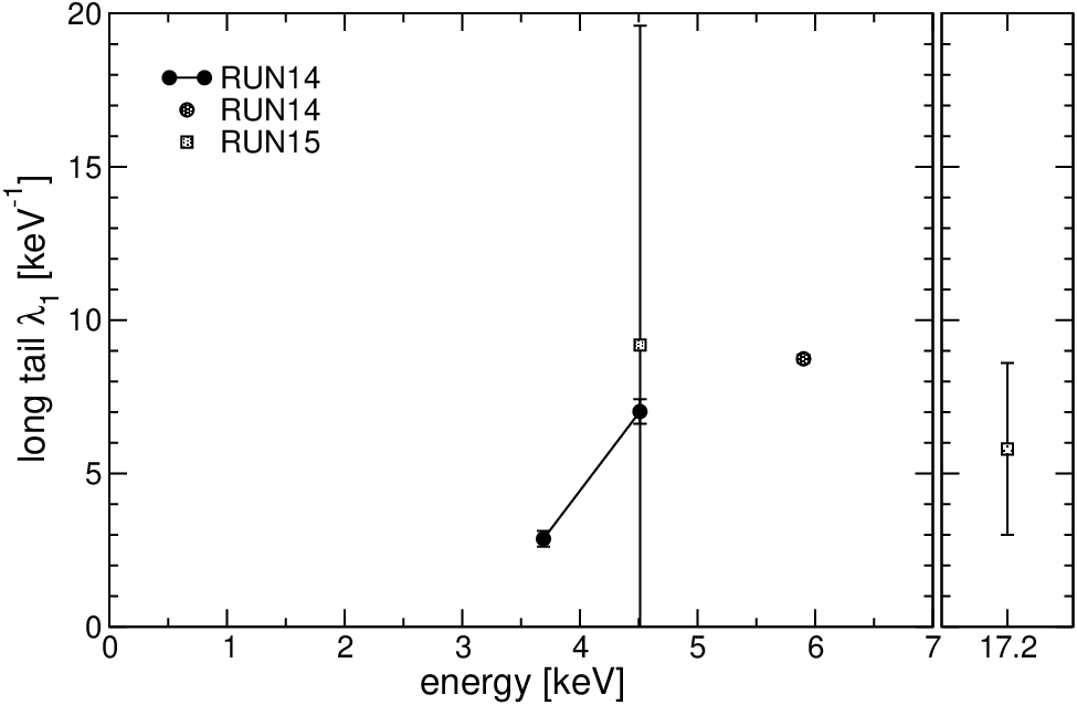
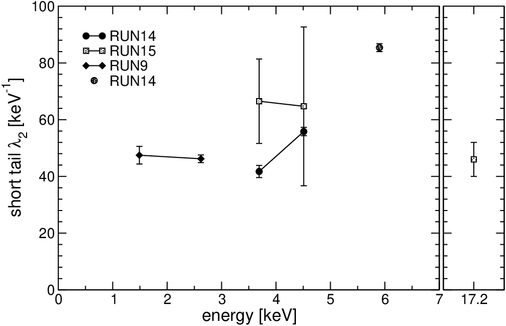


Figure 10, 10 and 10 show the results for the parameters , , , and as found by fitting the K peaks in the calibration spectra. In these plots the tail amplitudes and are normalized to the total peak area .
As far as the tail parameters are concerned, Figure 10 and 10 show the fit results only for a subset of the peaks we have analyzed. These results were selected considering the stability of the fit procedure with respect to the initial parameter values and to the energy interval as well as the convergence to meaningful values of all free parameters.
According to this considerations, a clean analysis of RUN14 data is possible only for the Ca, Ti and Mn peaks. As for the Cl peak, in the RUN14 spectrum the two M Pb peaks are too close for a correct estimation of the tail parameters (see spectrum in Figure 1), so the RUN9 spectrum was used instead. However, the low statistics and high background in this measurement prevent from properly estimating the long tail parameters, which are accordingly omitted in Figure 10 and 10. For the Al peak in RUN14, the determination of the long tail parameters is not possible because the peak shape has been altered by the software cuts applied to the data in order to separate spurious events from true beta decays (see [3] for details about the data analysis). Although in the analysis of RUN9 gentler offline cuts did not affect the shape of the Al peak, the long tail parameters are negatively influenced by the presence of the beta spectrum. Therefore, they are also omitted in Figure 10 and 10.
The results of the fits for the parameter are displayed in Figure 10. The parameter is the only one showing an evident trend with energy. Its energy dependency may be described by a sum of three squared contributions , where the constant term is the squared baseline width, i.e. the electronic noise contribution. We attribute the term to statistical fluctuations () in the thermalization of the AgReO4 and the term to uncorrected gain instabilities ().
The fit results for the other parameters are summarized in Figure 10 and 10. Concerning the Mn peak, a Compton back-scattering tail, as discussed in the previous section, accounts almost completely for the observed long tail. All other parameters are compatible with the hypothesis of no energy dependency. The safest conclusion is that, if any dependency exists at all, it is hidden by statistical and systematic errors or by the cross-correlations between the various parameters.
Because of the lower signal-to-background ratio in the RUN15 sum calibration spectrum, a satisfactory fit was possible only for the Ti K peak. As can be seen in Figure 10 and 10, both the long and short tail parameters are found to be compatible with the ones of RUN14. This is also illustrated in Figure 11 which shows the Ti K peaks in RUN14 and RUN15, normalized to overlay.

For what concerns the escape peaks in RUN15, the analysis has been restricted to the Re K escape peaks since the K escape peaks show a too complex structure (see Figures 5 and 6). The Re K escape peaks have been fitted fixing their natural widths and asymmetry indexes , according to the data in Table 4. Fits have been performed with the two tails as in (8) as well as with one or no tail, both on the K1 alone and on the two K peaks together. The results are listed in Table 5 and shown in Figure 12 for the two K peaks.
| K and K escape peaks | |||||
|---|---|---|---|---|---|
| Peak | |||||
| model | [%] | [keV-1] | [%] | [keV-1] | |
| no tail | – | – | – | – | 1.408 |
| 1 tail | – | – | 1.224 | ||
| 2 tails | 1.210 | ||||
Although the fits with the three models are almost undistinguishable by eye, the suggests that the one without tails is the least satisfactory. The two tail and one tail model fits have very similar , although the best fit is obtained with the two tail model.
The results for the K1 escape peak fit are compared with the ones for the low energy peaks in Figure 10 and 10. The comparison confirms that the parameters do not depend strongly on the energy. Considering instead the tail amplitudes, it may be concluded that, for the uniformly distributed escape events, whereas the long tail is clearly reduced – as expected for a surface effect –, the short tail is considerably higher than for the low energy peaks. However, it is worth noting that the short tail amplitude determination is hindered by the large escape peak width together with the limited statistics, as shown by the large error in Table 5.


4 Montecarlo Simulations
To understand the origin of the observed tails another Montecarlo simulation based on the Geant4 toolkit was developed. Hereby each X-ray line was simulated separately using the energies and line widths listed in Tables 3 and 4, respectively. An additional exponential tail was added to the left of the Mn lines according to the results shown in Figure 4. For the simulation of the Re K escape lines, the initial 44Ti -line at keV was used; the escape lines are then automatically generated by the Montecarlo simulation. To account for the energy resolution of the detector and compare with experimental data, the resulting energy spectra were convoluted with a Gaussian, whose was taken from the fitting of the respective line. As the AgReO4 crystals do not have a regular geometrical shape [3, 17], they were approximated by a cylinder with a diameter of m and a thickness of m.
In addition to the summed spectrum, the sum of the two channels 5 and 6 was investigated separately, because only these two channels were used for the escape peak analysis.
The Montecarlo simulation describes creation, transport and interaction of the initial photo-electron created by the X-ray photon, of the secondary electrons as well as of the secondary X-rays. However, it does not describe the energy transfer from the electron(s) to the phonon system which ultimately produces the signal observed with thermal detectors. Incomplete energy detection that creates a low energy tail can be caused by either incomplete energy transfer from the electrons to the phonon system, or by a reduced temperature signal due to phonon energy losses or energy deposition in thermally weakly-coupled volumes.
As the Montecarlo simulation does not account for these different processes, the energy deposited by the electron(s) in each Montecarlo step was multiplied by a weight function , where is the position at which the energy deposition happens.


As the fitting function could be divided into a long and a short shoulder, we have used a function according to a model with two loss mechanisms. The first one assumes that the AgReO4 crystal has an insensitive surface layer of thickness . The electron energy deposited in this layer does not contribute entirely to the thermal signal because of an incomplete conversion into phonons. The transition from insensitive to sensitive volume is smooth and described by a diffusion profile with a diffusion length : 33 3 The choice of this function clearly determines the exact tail shape. With the present choice the shape will be only approximately exponential, but the natural linewidth , the noise and the statistics prevent from appreciating the difference.
| (10) |
The result of this simulation is displayed in Figure 13 for the case of RUN14. The and parameters were found by one-dimensional analysis to reproduce the experimental data in the 1.0 – 7.0 keV energy interval and are reported in Table 6. It is shown clearly in Figure 13 that this simple model can describe the long shoulders sufficiently well, although it fails to account for the short shoulders.
| run | RUN14 | RUN14 | RUN15 |
|---|---|---|---|
| spectrum | sum | channel 5+6 | channel 5+6 |
| [nm] | 20 | 52 | 52 |
| [nm] | 64 | 52 | 52 |
| [m] | 279 | 280 | 280 |
| [m] | 1 | 1 | 1 |
| L | 0.010 | 0.010 | 0.010 |


The K peaks in the Montecarlo simulated spectrum (Figure 13) were fitted with one single exponential tail and the resulting long tail amplitudes and parameters are plotted in Figure 14 together with the results shown in Figure 10 and 10. The comparison confirms that this simple model indeed reproduces the features of the experimental data and, as expected for a surface effect, the long tail disappears almost completely in the escape peaks.
As the short tail parameters and show a completely different dependence on the energy, another mechanism must be found to explain the short component of the experimental peaks. Two types of effects can be the origin of the observed short tail. The first one consists of spatial effects, where the tail depends on the energy because the spatial distribution of the interaction does. All effects which are not related to the interaction position belong to the second type.
In fact there are good reasons to suspect the presence of volume effects that are caused by the dependence of the thermal signal on the interaction position. The calorimeter is a composite object with an absorber crystal and a thermometer attached to it by means of a small glue spot. If the phonons do not reach complete thermal equilibrium in the whole absorber crystal faster than the detector thermal time constant, part of them will be lost depending on the X-ray impact location44 4 Indeed the pulses observed with our AgReO4 microcalorimeters cannot be understood only as thermal signals. In general they present two decay time constants. The longer one – few tens of milliseconds – could be interpreted as the detector thermal relaxation to the operating temperature. The shorter one – few milliseconds – is probably caused by the direct interaction of out-of-equilibrium phonons in the attached silicon thermometer.. It is reasonable to assume that impact locations farther away from the attachment point of the thermometer will create a reduced thermal signal, thus creating a local dependence of the energy response.
Therefore, as an example for this loss mechanism, we report here on one model which has a dependence on the distance of the energy deposition from the attachment point of the thermometer. To account for a smooth transition of sensitivity, we used a second diffusion model:
| (11) |
where stands for the distance of the impact location from the attachment point (see Figure 15 for a schematic description), is a “thickness” parameter describing the gradual decrease of sensitivity for crystal regions farther away from the attachment point, and describes the transition width. sets the minimum value for the limit: when , approaches 0 for .
The final weighting function is then given by
| (12) |


The parameters used in the simulations are summarized in Table 6: these parameters correspond to a weight function which is 1.0 in the whole crystal volume and decreases just on the lower rim of the cylindrical crystal (see Figure 15). Figure 16 shows the result of the simulated spectrum compared with the measured spectrum from Figure 1.
From the values of the simulation parameters, it can also be deduced that the two mechanisms have different origin. Whereas and are rather different for the sum of all and the sum of only two channels, this cannot be said for the other parameters , and . This strengthens our interpretation of the first mechanism as a surface effect which is expected to be individual for each crystal. The similarity of the other parameters for the different channels points to a more systematic effect common to all crystals.


Figure 17 shows the measured as well as the simulated Re K escape peaks for the 44Ti measurement (RUN15). The Re K escape peaks were simulated with the same values for , and as for the calibration peaks, adding an increased low-energy background from the 44Ti source. The agreement between the experiment and Montecarlo as shown in the left panel of Figure 17 is fairly good. The right panel of Figure 17 shows the escape peaks obtained with the Montecarlo simulation when neither the transition natural width nor the detector resolution are included: the plot shows that although no appreciable long term tail is expected a very small short term component is indeed present in the simulation. However, a comparison with the results in Table 5 and Figure 10 shows that the Montecarlo fails to predict the correct amplitude of this short tail by more than an order of magnitude.
A model that depends on the distance of the interaction point from the calorimeter is naturally more dependent on the geometrical shape of the crystal than a surface model. However, other models for spatial dependence with different assumptions for the geometry as well as for the weighting function show similar shortcomings.
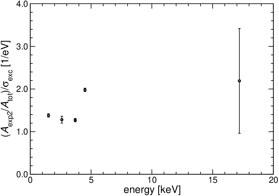
The second type of effects which can cause a tail may include, for example, complex energy losses due to trapping in metastable states, event pile-up as well as other analysis artefacts. In particular, for what concerns these effects, it is quite intriguing to notice that the short tail amplitude and the line width vary with the energy in a similar way. This is illustrated in Figure 19 where the ratio between the relative amplitude and the peak broadening in excess of the baseline width () is plotted versus the energy. A common energy dependence might be inferred from this plot. This points to a possible common explanation for the two peak parameters.
Indeed both the above types of effects could be present in our detectors. However, with our current understanding it is not possible to build models that satisfactory explain the short tail in our data. A better understanding of the mechanisms causing that short tail would require a higher statistics measurement with the 44Ti source as well as calibrations with lower energy (i.e. keV) or X-ray sources to better investigate the tail energy – and therefore spatial – dependence.
The important aim of the present investigation was to determine to which extent the tails observed in the calibration peaks affect the beta spectrum as well. Unfortunately nothing conclusive was found for the short tail. Therefore in order to evaluate the detector response function expected for an internal uniformly distributed 2.5 keV beta, the Montecarlo was run with few different assumptions about the mechanism causing the tail.
Figure 18 shows the results. For sake of comparison, in the left panel, the Montecarlo simulation was run for an external 2.5 keV X-ray with the simple surface effect model in (10) alone (light grey histogram) and with an additional short tail (darker histogram) with the parameters found for the Cl K X-ray line (see Figure 10 and 10), i.e. for instance with an amplitude of about 10%. The simulations for the internal uniformly distributed 2.5 keV beta are shown in the right panel. The simple surface model is the light grey histogram at the bottom: the internal beta response function still presents a tail due to a small fraction of beta interactions close to the surface, but its amplitude is about a factor 100 smaller than for the external X-ray. The darker histograms correspond to two hypotheses for the short tail origin. The black one is caused by a volume effect and therefore the tail amplitude is taken as found for the Re K escape peaks (about 70%). The dark grey one is for a non-spatial effect; therefore, it is only energy dependent and characterized by the same values found as for the external X-rays. In both panels, the purely Gaussian peak expected at this energy is plotted for reference (solid line).
The effect of the long tail in the beta response function is negligible for an experiment like MIBETA. As far as the short tail is concerned, the relevance for MIBETA depends of course on which is the correct modeling. This lack of knowledge has therefore to be treated as a source of systematic uncertainty and correctly quantified. The effect of the tails on upcoming higher statistics experiments will need a deeper analysis.
5 Conclusions
In this paper we have described a function which allows a satisfactory interpolation of the peaks observed in the calibration spectra of the MIBETA experiment.
The results of the fitting show that at least the longer of the two exponential tails towards low energy may be indeed understood as a result of a surface effect. This is confirmed by the Rhenium escape peaks which have a strongly reduced long tail. We convincingly tested the surface effect hypothesis with a simple Montecarlo simulation. We used a simple phenomenological model which does not pretend to account realistically for the complex details of electron and phonon interactions. Nevertheless the simulation proves that a surface effect as the one described by (10) can explain the observed peak shape, no matter what is the underlying physics.
On the other hand, the shorter of the two exponentials cannot be understood with a simple assumption. A geometrical effect of the crystal shape may play a role, but for now we can only conclude that we have no convincing description of this effect.
Further investigations with a larger number of regularly shaped crystals as of in MARE-1 will be mandatory to clarify this situation.
6 Acknowledgments
We would like to thank Prof. E. B. Norman at Lawrence Berkeley National Laboratory for providing us with the 44Ti source used for this work.
References
- (1) Editor C. Enss, Cryogenic Particle Detection (Springer, Berlin, 2005)
- (2) C. Arnaboldi et al., Phys. Rev. Lett. 91, 161802 (2003).
- (3) M. Sisti et al., Nucl. Instrum. Methods A 520, 125 (2004).
- (4) F. Gatti, Nucl. Phys. B 91, 293 (2001).
- (5) M. Galeazzi et al., Phys. Rev. C 63, 014302 (2001).
- (6) G. Zchornack, Handbook of X-Ray Data (Springer Berlin Heidelberg New York 2007)
- (7) https://geant4.web.cern.ch/geant4/ and the “Physics Reference Manual” therein.
- (8) C. J. Bland, Appl. Radiat. Isot. 49 (1998) 1225
- (9) G. Bortels and P. Collaers, Appl. Radiat. Isot. 38 (1987) 831;
- (10) S. Doniach and M. Sunjic, J. Phys. C 3 (1970) 285
- (11) J. Kawai et al., Phys. Rev. Lett. 57 (1986) 988
- (12) J. Kawai et al., Phys. Rev. A 39 (1989) 3686
- (13) G. Hölzner et al., Phys. Rev. A 56 (1997) 4554
- (14) L. G. Parratt, Phys. Rev. 50 (1936) 1
- (15) M. O. Krause and J. H. Oliver, J. Phys. Chem. Ref. Data 8 (1979) 329
- (16) P. Citrin et al., Phys. Rev. B 10 (1974) 1762
- (17) A. Nucciotti et al. in Proceedings on the 9th International Workshop on Low Temperature Detectors, F. S. Porter et al. (eds.), AIP Conference Proceedings 605 (2002) 453