跳到论文正文
W Papers独立论文阅读器 arXiv:1210.5340 论文正文 计算阅读时间 · 0%
引用这篇论文根据当前论文元数据生成,正式投稿前建议核对。


License: arXiv.org perpetual non-exclusive license
arXiv:1210.5340v1 [quant-ph] 19 Oct 2012

Entanglement dynamics for qubits dissipating into a common environment

Laleh Memarzadeh Note: email: memarzadeh@sharif.edu Affiliation: Department of Physics, Sharif University of Technology, Teheran, Iran    Stefano Mancini Note: email: stefano.mancini@unicam.it Affiliation: School of Science and Technology, University of Camerino, I-62032 Camerino, Italy Affiliation: INFN-Sezione di Perugia, I-06123 Perugia, Italy
Abstract

We provide an analytical investigation of the entanglement dynamics for a system composed of an arbitrary number of qubits dissipating into a common environment. Specifically we consider initial states whose evolution remains confined on low dimensional subspaces of the operators space. We then find for which pairs of qubits entanglement can be generated and can persist at steady state. Finally, we determine the stationary distribution of entanglement as well as its scaling versus the total number of qubits in the system.

pacs
03.67.Bg, 03.65.Yz

I Introduction

Entanglement is synonymous of quantum correlations that cannot be explained by any local classical theory. Initially this notion was relegated to foundational issues, but in the last decades it has pervaded quantum information and other areas of physics [1]. Being a purely quantum phenomenon it was considered fragile under contamination of environment noise in open quantum systems. Nevertheless, in recent years it has been shown that it can persist for long time up to stationary conditions in several contexts [2] (see also [3] for a striking experiment on long living entanglement). More importantly it has been shown that the environment can play a constructive role in establishing entanglement [4, 5]. Quite remarkably it happens that even without any interaction among subsystems a common dissipative environment is able to induce entanglement [5]. However, this possibility has been proved true only for systems composed by two subsystems due to technical difficulties arising when accounting for more subsystems.

Here we overcome these difficulties and achieve results for an arbitrary number of subsystems by considering a limited number of initially available excitations and by exploiting a power expansion for the dissipation superoperator. This allows us to restrict the analysis to a low dimensional subspace of the operators space.

We find that pairwise entanglement is not created at any time between initially excited qubits. Instead, it is created and persists at steady state for pairs of initially excited and initially not excited qubits. The same holds true for pairs of qubits initially in the ground state, but in such a case the amount of entanglement is negligibly smaller than the previous case.

II System Dynamics

Let us consider a system of nn qubits with associated Hilbert space ℋ≃ℂ2⊗n\mathcal{H}\simeq\mathbb{C}^{2\otimes n}. Let {|0⟩,|1⟩}⊗n\{|0\rangle,|1\rangle\}^{\otimes n} be the orthonormal basis, with |0⟩|0\rangle (resp. |1⟩|1\rangle) the ground (resp. excited) single qubit state.

We want to study the dynamics of this system of qubits when they dissipate together into an environment at zero temperature. It will be governed by the Lindblad master equation [6]:

ρ˙​(t)=2​σ​ρ​(t)​σ†−σ†​σ​ρ​(t)−ρ⁡(t)​σ†​σ≡𝒟​ρ​(t),\dot{\rho}(t)=2\sigma\rho(t)\sigma^{{\dagger}}-\sigma^{\dagger}\sigma\rho(t)-\rho(t)\sigma^{\dagger}\sigma\equiv\mathcal{D}\rho(t), (1)

where

σ:=∑i=1nσi,\sigma:=\sum_{i=1}^{n}\sigma_{i}, (2)

with σi:=|0⟩​⟨1|\sigma_{i}:=|0\rangle\langle 1| for the iith qubit. The dissipation rate has been set equal to 11 for the sake of simplicity.

Let us describe the strategy we will put into practice to solve (1). The fomal solution reads ρ⁡(t)=et​𝒟​ρ​(0)\rho(t)=e^{t\mathcal{D}}\rho(0). To explicitly find ρ⁡(t)\rho(t) let us first write the Taylor expansion:

ρ⁡(t)=ρ⁡(0)+t​𝒟​ρ​(0)+t22!​𝒟2​ρ​(0)+t33!​𝒟3​ρ​(0)+⋯.\rho(t)=\rho(0)+t\mathcal{D}\rho(0)+\frac{t^{2}}{2!}\mathcal{D}^{2}\rho(0)+\frac{t^{3}}{3!}\mathcal{D}^{3}\rho(0)+\cdots. (3)

Now notice that once the initial state ρ⁡(0)\rho(0) has been chosen, the dynamics (being purely dissipative at zero temperature) can only decrease the number of initial excitation present in ρ⁡(0)\rho(0). That is, repeated applications of 𝒟\mathcal{D} to ρ⁡(0)\rho(0) will leave the state within a subspace ℍρ⁡(0)⊂ℍ\mathbb{H}_{\rho(0)}\subset\mathbb{H} of the Hilbert space ℍ=ℋ⊗ℋ∗\mathbb{H}=\mathcal{H}\otimes\mathcal{H}^{*} where ℋ∗\mathcal{H}^{*} stands for the dual of ℋ\mathcal{H}. After having identified ℍρ⁡(0)\mathbb{H}_{\rho(0)}, i.e. a set of operators on ℋ\mathcal{H} spanning ℍρ⁡(0)\mathbb{H}_{\rho(0)}, we will write down ρ⁡(0)\rho(0) as linear combination of such operators with unknown time dependent coefficients. Then, by inserting this expansion into Eq.(1) we will derive a set of linear differential equations for the unknown coefficients. In this way if the initial state contains a small number of excitation we can hope to provide an analytical solution. In fact given a number of initial excitations ee (e≪ne\ll n) the following inequality holds true:

d​i​m​ℍρ⁡(0)≤(2e)2≪(2n)2=d​i​m​ℍ.dim\mathbb{H}_{\rho(0)}\leq\left(2^{e}\right)^{2}\ll\left(2^{n}\right)^{2}=dim\mathbb{H}. (4)

Finally, notice that (1) does not satisfy the condition for the uniqueness of a stationary solution. This condition requires that the only operators commuting with the Lindblad operator σ\sigma must be multiples of identity [7]. Hence we should expect different steady states depending on the choice of ρ⁡(0)\rho(0).

III One initial excitation (e=1e=1)

In this section we assume that initially only the kkth qubit is in the excited state while all the others are in the ground state. Let us denote this state as |k⟩|k\rangle, then ρ⁡(0)=|k⟩​⟨k|\rho(0)=|k\rangle\langle k|.

By applying 𝒟\mathcal{D} to ρ⁡(0)=|k⟩​⟨k|\rho(0)=|k\rangle\langle k| we can easily find the following closed relations:

𝒟​|k⟩​⟨k|\displaystyle\mathcal{D}|k\rangle\langle k| =\displaystyle= 2​|G⟩​⟨G|−(|Ek̸⟩​⟨k|+|k⟩​⟨Ek̸|),\displaystyle 2|G\rangle\langle G|-(|E_{\not k}\rangle\langle k|+|k\rangle\langle E_{\not k}|),
𝒟​|G⟩​⟨G|\displaystyle\mathcal{D}|G\rangle\langle G| =\displaystyle= 0,\displaystyle 0,
𝒟⁡(|Ek̸⟩​⟨k|+|k⟩​⟨Ek̸|)\displaystyle\mathcal{D}\left(|E_{\not k}\rangle\langle k|+|k\rangle\langle E_{\not k}|\right) =\displaystyle= 4​(n−1)​|G⟩​⟨G|−2|Ek̸⟩​⟨Ek̸|\displaystyle 4(n-1)|G\rangle\langle G|-2|E_{\not k}\rangle\langle E_{\not k}|
−2​(n−1)​|k⟩​⟨k|\displaystyle-2(n-1)|k\rangle\langle k|
−n⁡(|Ek̸⟩​⟨k|+|k⟩​⟨Ek̸|),\displaystyle-n(|E_{\not k}\rangle\langle k|+|k\rangle\langle E_{\not k}|),
𝒟⁡|Ek̸⟩​⟨Ek̸|\displaystyle\mathcal{D}|E_{\not k}\rangle\langle E_{\not k}| =\displaystyle= 2​(n−1)2​|G⟩​⟨G|\displaystyle 2(n-1)^{2}|G\rangle\langle G|
−2​(n−1)​|Ek̸⟩​⟨Ek̸|\displaystyle-2(n-1)|E_{\not k}\rangle\langle E_{\not k}|
−(n−1)​(|Ek̸⟩​⟨k|+|k⟩​⟨Ek̸|),\displaystyle-(n-1)(|E_{\not k}\rangle\langle k|+|k\rangle\langle E_{\not k}|),

where we have defined

|G⟩:=|0⟩⊗n,|Ek̸⟩:=∑i≠kn|i⟩,\displaystyle|G\rangle:=|0\rangle^{\otimes n},\qquad|E_{\not k}\rangle:=\sum_{i\neq k}^{n}|i\rangle, (6)

(|i⟩|i\rangle stands for a state in which the iith qubit is in the excited state and all the others are in the ground state).

With the help of Eq.() we identify the subspace

ℍρ⁡(0)\displaystyle\mathbb{H}_{\rho(0)} =\displaystyle= span{|G⟩⟨G|,|k⟩⟨k|,|Ek̸⟩⟨Ek̸|,\displaystyle span\left\{|G\rangle\langle G|,|k\rangle\langle k|,|E_{\not k}\rangle\langle E_{\not k}|,\right. (7)
(|Ek̸⟩⟨k|+|k⟩⟨Ek̸|)}.\displaystyle\left.\hskip 28.45274pt(|E_{\not k}\rangle\langle k|+|k\rangle\langle E_{\not k}|)\right\}.

Then we can write

ρ⁡(t)\displaystyle\rho(t) =\displaystyle= a0​(t)​|G⟩​⟨G|+a1​(t)|k⟩​⟨k|+a2​(t)|Ek̸⟩​⟨Ek̸|\displaystyle a_{0}(t)|G\rangle\langle G|+a_{1}(t)|k\rangle\langle k|+a_{2}(t)|E_{\not k}\rangle\langle E_{\not k}| (8)
+a3​(t)​(|Ek̸⟩​⟨k|+|k⟩​⟨Ek̸|),\displaystyle+a_{3}(t)(|E_{\not k}\rangle\langle k|+|k\rangle\langle E_{\not k}|),

which, upon insertion into (1), leads to the set of differential equations

a˙0\displaystyle\dot{a}_{0} =\displaystyle= 2​a1+2​(n−1)2​a2+4​(n−1)​a3,\displaystyle 2a_{1}+2(n-1)^{2}a_{2}+4(n-1)a_{3},
a˙1\displaystyle\dot{a}_{1} =\displaystyle= −2​a1−2​(n−1)​a3,\displaystyle-2a_{1}-2(n-1)a_{3},
a˙2\displaystyle\dot{a}_{2} =\displaystyle= −2​(n−1)​a2−2​a3,\displaystyle-2(n-1)a_{2}-2a_{3},
a˙3\displaystyle\dot{a}_{3} =\displaystyle= −a1−(n−1)​a2−n​a3,\displaystyle-a_{1}-(n-1)a_{2}-na_{3}, (9)

with initial conditions a0​(0)=a2​(0)=a3​(0)=0,a1​(0)=1a_{0}(0)=a_{2}(0)=a_{3}(0)=0,a_{1}(0)=1.

Solving them we arrive at the density operator

ρ⁡(t)\displaystyle\rho(t) =\displaystyle= (1−f⁡(t))2​|k⟩​⟨k|+f⁡(t)​(2−n​f​(t))|G⟩​⟨G|\displaystyle(1-f(t))^{2}|k\rangle\langle k|+f(t)(2-nf(t))|G\rangle\langle G| (10)
+f​(t)2​|Ek̸⟩​⟨Ek̸|\displaystyle+f(t)^{2}|E_{\not k}\rangle\langle E_{\not k}|
−f⁡(t)​(1−f⁡(t))​(|Ek̸⟩​⟨k|+|k⟩​⟨Ek̸|),\displaystyle-f(t)(1-f(t))(|E_{\not k}\rangle\langle k|+|k\rangle\langle E_{\not k}|),

where f⁡(t):=1n​(1−e−n​t)f(t):=\frac{1}{n}(1-e^{-nt}).

To analyze the pairwise entanglement between the qubit kk and a generic other qubit jj we compute the partial trace of (10) overall the other qubits and obtain the following density operator

ρk,j\displaystyle\rho_{k,j} =\displaystyle= (1−f⁡(t))2​|10⟩​⟨10|+f2​(t)|01⟩​⟨01|\displaystyle(1-f(t))^{2}|10\rangle\langle 10|+f^{2}(t)|01\rangle\langle 01|
−f⁡(t)​(1−f⁡(t))​(|10⟩​⟨01|+|01⟩​⟨10|−2|00⟩​⟨00|).\displaystyle-f(t)(1-f(t))\left(|10\rangle\langle 01|+|01\rangle\langle 10|-2|00\rangle\langle 00|\right).

Using the concurrence [8] as a measure of entanglement of ρk,j\rho_{k,j} in Eq.() we find its time evolution as

Ck,j​(t)=2n​(1−e−n​t)​(1−1−e−n​tn).C_{k,j}(t)=\frac{2}{n}\left(1-e^{-nt}\right)\left(1-\frac{1-e^{-nt}}{n}\right). (12)

As it is shown in Fig.1, entanglement is generated between the kkth qubit (initially in the excited state) and an arbitrary qubit jj (initially in the ground state), although there is no direct interaction between them. The maximum amount of entanglement decreases with the system size nn, but the concurrence achieves its maximum value faster when the system size is larger.

Refer to caption
Figure 1: Concurrence Ck,jC_{k,j} versus time tt. From top to bottom the system size is n=2,6,10,14n=2,6,10,14.

Letting tt going to infinity in Eq.(12) we can find the behavior of stationary entanglement versus the system size nn as

Ck,j​(∞)=2​(n−1)n2.C_{k,j}(\infty)=\frac{2(n-1)}{n^{2}}. (13)

This is shown in Fig.2.

Refer to caption
Figure 2: Stationary concurrence Ck,jC_{k,j} versus system size nn.

To study the entanglement between any two qubits initially in the ground state, we compute the reduced density matrix of jjth and mmth qubits (j,m≠kj,m\neq k). By referring to Eq.(10) it is easy to show that

ρj,m\displaystyle\rho_{j,m} =\displaystyle= (1−2​f2​(t))​|00⟩​⟨00|\displaystyle\left(1-2f^{2}(t)\right)|00\rangle\langle 00| (14)
+f2(t)(|10⟩+|01⟩)((⟨10|+⟨01|).\displaystyle+f^{2}(t)\left(|10\rangle+|01\rangle\right)(\left(\langle 10|+\langle 01|\right).

The concurrence [8] of ρj,m\rho_{j,m} in Eq.(14) results

Cj,m(t)=2(1−e−n​tn)2.C_{{}_{j,m}}(t)=2\left(\frac{1-e^{-nt}}{n}\right)^{2}. (15)

Its behavior is shown in Fig.3. From Eq.(15) it is easy to see that at steady state it is Cj,m​(∞)=2n2C_{j,m}(\infty)=\frac{2}{n^{2}}, which is negligible compared to Ck,j​(∞)C_{k,j}(\infty) for large nn. Therefore for large systems, we have a star graph (see Fig.4) as steady state.

Refer to caption
Figure 3: Concurrence Cj,mC_{j,m} versus time tt. From top to bottom the system size is n=2,6,10,14n=2,6,10,14.
Refer to caption
Figure 4: Pictorial representation of the leading stationary correlations (edges) among qubits (circles). Red (reps. blue) circles represents qubits initially in the excited (resp. ground) state.

IV Two initial excitations (e=2e=2)

In this section we assume that initially two qubits, say the kkth and the llth, are in the excited state, while all the others are in the ground state. Let us denote this state as |k,l⟩|k,l\rangle, then ρ(0)=|k,l⟩⟨k,l|\rho(0)=|k,l\rangle\langle k,l|.

By applying 𝒟\mathcal{D} to ρ(0)=|k,l⟩⟨k,l|\rho(0)=|k,l\rangle\langle k,l| we can find the following closed relations:

𝒟|k,l⟩⟨k,l|\displaystyle\mathcal{D}|k,l\rangle\langle k,l| =\displaystyle= 2|k+l⟩⟨k+l|−4|k,l⟩⟨k,l|−Λ,\displaystyle 2|k+l\rangle\langle k+l|-4|k,l\rangle\langle k,l|-\Lambda,
𝒟​|k+l⟩​⟨k+l|\displaystyle\mathcal{D}|k+l\rangle\langle k+l| =\displaystyle= 8​|G⟩​⟨G|−2​Ω−4|k+l⟩​⟨k+l|,\displaystyle 8|G\rangle\langle G|-2\Omega-4|k+l\rangle\langle k+l|,
𝒟​|G⟩​⟨G|\displaystyle\mathcal{D}|G\rangle\langle G| =\displaystyle= 0,\displaystyle 0,
𝒟​Ω\displaystyle\mathcal{D}\Omega =\displaystyle= 2​(n−2)​(4​|G⟩​⟨G|−|k+l⟩​⟨k+l|)−n​Ω−4​|Ek̸​l̸⟩​⟨Ek̸​l̸|,\displaystyle 2(n-2)\left(4|G\rangle\langle G|-|k+l\rangle\langle k+l|\right)-n\Omega-4|E_{\not k\not l}\rangle\langle E_{\not k\not l}|,
𝒟⁡|Ek̸​l̸⟩​⟨Ek̸​l̸|\displaystyle\mathcal{D}|E_{\not k\not l}\rangle\langle E_{\not k\not l}| =\displaystyle= (n−2)​(2​(n−2)​|G⟩​⟨G|−Ω−2|Ek̸​l̸⟩​⟨Ek̸​l̸|),\displaystyle(n-2)\left(2(n-2)|G\rangle\langle G|-\Omega-2|E_{\not k\not l}\rangle\langle E_{\not k\not l}|\right),
𝒟​Λ\displaystyle\mathcal{D}\Lambda =\displaystyle= 4(n−2)(|k+l⟩⟨k+l|−|k,l⟩⟨k,l|)−2|B⟩⟨B|+4(Ω−Π)−(n+2)Λ,\displaystyle 4(n-2)\left(|k+l\rangle\langle k+l|-|k,l\rangle\langle k,l|\right)-2|B\rangle\langle B|+4(\Omega-\Pi)-(n+2)\Lambda,
𝒟​|B⟩​⟨B|\displaystyle\mathcal{D}|B\rangle\langle B| =\displaystyle= 2​(n−2)2​|k+l⟩​⟨k+l|+2​(n−2)​(2​Ω−Λ)+8|Ek̸​l̸⟩​⟨Ek̸​l̸|−2​n|B⟩​⟨B|−4​Γ,\displaystyle 2(n-2)^{2}|k+l\rangle\langle k+l|+2(n-2)(2\Omega-\Lambda)+8|E_{\not k\not l}\rangle\langle E_{\not k\not l}|-2n|B\rangle\langle B|-4\Gamma,
𝒟​Π\displaystyle\mathcal{D}\Pi =\displaystyle= (n−3)​(2​Ω−Λ)−2​(n−2)​Π−Γ,\displaystyle(n-3)\left(2\Omega-\Lambda\right)-2(n-2)\Pi-\Gamma,
𝒟​Γ\displaystyle\mathcal{D}\Gamma =\displaystyle= 2​(n−3)​(4​|Ek̸​l̸⟩​⟨Ek̸​l̸|−|B⟩​⟨B|)+2​(n−2)​(n−3)​Ω−8​|H⟩​⟨H|−2​(n−2)​Π−3​(n−2)​Γ,\displaystyle 2(n-3)\left(4|E_{\not k\not l}\rangle\langle E_{\not k\not l}|-|B\rangle\langle B|\right)+2(n-2)(n-3)\Omega-8|H\rangle\langle H|-2(n-2)\Pi-3(n-2)\Gamma,
𝒟​|H⟩​⟨H|\displaystyle\mathcal{D}|H\rangle\langle H| =\displaystyle= (n−3)​(2​(n−3)​|Ek̸​l̸⟩​⟨Ek̸​l̸|−4|H⟩​⟨H|−Γ),\displaystyle(n-3)\left(2(n-3)|E_{\not k\not l}\rangle\langle E_{\not k\not l}|-4|H\rangle\langle H|-\Gamma\right), (16)

where, in addition to Eq.(6), we have defined

|k+l⟩\displaystyle|k+l\rangle :⁣=\displaystyle:= |k⟩+|l⟩,\displaystyle|k\rangle+|l\rangle,
|Ek̸​l̸⟩\displaystyle|E_{\not k\not l}\rangle :⁣=\displaystyle:= ∑i≠k,ln|i⟩,\displaystyle\sum_{i\neq k,l}^{n}|i\rangle,
|B⟩\displaystyle|B\rangle :⁣=\displaystyle:= ∑i≠k|i,k⟩+∑i≠l|i,l⟩,\displaystyle\sum_{i\neq k}|i,k\rangle+\sum_{i\neq l}|i,l\rangle,
|H⟩\displaystyle|H\rangle :⁣=\displaystyle:= ∑h>i|h,i⟩,h,i≠k,l,\displaystyle\sum_{h>i}|h,i\rangle,\hskip 56.9055pth,i\neq k,l,

and

Ω\displaystyle\Omega :⁣=\displaystyle:= |Ek̸​l̸⟩​⟨k+l|+|k+l⟩​⟨Ek̸​l̸|,\displaystyle|E_{\not k\not l}\rangle\langle k+l|+|k+l\rangle\langle E_{\not k\not l}|,
Λ\displaystyle\Lambda :⁣=\displaystyle:= |B⟩⟨k,l|+|k,l⟩⟨B|,\displaystyle|B\rangle\langle k,l|+|k,l\rangle\langle B|,
Π\displaystyle\Pi :⁣=\displaystyle:= |H⟩⟨k,l|+|k,l⟩⟨H|,\displaystyle|H\rangle\langle k,l|+|k,l\rangle\langle H|,
Γ\displaystyle\Gamma :⁣=\displaystyle:= |B⟩​⟨H|+|H⟩​⟨B|.\displaystyle|B\rangle\langle H|+|H\rangle\langle B|. (18)

With the help of Eq.(16) we can identify the subspace

ℍρ⁡(0)\displaystyle\mathbb{H}_{\rho(0)} =\displaystyle= span{|G⟩⟨G|,|Ek̸​l̸⟩⟨Ek̸​l̸|,|k+l⟩⟨k+l|,Ω,\displaystyle span\left\{|G\rangle\langle G|,|E_{\not k\not l}\rangle\langle E_{\not k\not l}|,|k+l\rangle\langle k+l|,\Omega,\right.
|k,l⟩⟨k,l|,|B⟩⟨B|,|H⟩⟨H|,Λ,Π,Γ}.\displaystyle\left.\hskip 28.45274pt|k,l\rangle\langle k,l|,|B\rangle\langle B|,|H\rangle\langle H|,\Lambda,\Pi,\Gamma\right\}.

Then we can write

ρ⁡(t)\displaystyle\rho(t) =\displaystyle= b0​(t)​|G⟩​⟨G|+b1​(t)|Ek̸​l̸⟩​⟨Ek̸​l̸|+b2​(t)|k+l⟩​⟨k+l|\displaystyle b_{0}(t)|G\rangle\langle G|+b_{1}(t)|E_{\not k\not l}\rangle\langle E_{\not k\not l}|+b_{2}(t)|k+l\rangle\langle k+l| (20)
+b3(t)Ω+b4(t)|k,l⟩⟨k,l|+b5(t)|B⟩⟨B|\displaystyle+b_{3}(t)\Omega+b_{4}(t)|k,l\rangle\langle k,l|+b_{5}(t)|B\rangle\langle B|
+b6​(t)​|H⟩​⟨H|+b7​(t)​Λ+b8​(t)​Π+b9​(t)​Γ.\displaystyle+b_{6}(t)|H\rangle\langle H|+b_{7}(t)\Lambda+b_{8}(t)\Pi+b_{9}(t)\Gamma.

By inserting this expansion of ρ⁡(t)\rho(t) into Eq.(1) we arrive at the following set of differential equations:

b˙0​(t)\displaystyle\dot{b}_{0}(t) =\displaystyle= 2​(n−2)2​b1​(t)+8​b2​(t)+8​(n−2)​b3​(t),\displaystyle 2(n-2)^{2}b_{1}(t)+8b_{2}(t)+8(n-2)b_{3}(t), (21)
𝐯˙​(t)\displaystyle\dot{\bf v}(t) =\displaystyle= M​𝐯​(t),\displaystyle M{\bf v}(t), (22)

where 𝐯=(b1,b2,b3,b4,b5,b6,b7,b8,b9)𝖳{\bf{v}}=(b_{1},b_{2},b_{3},b_{4},b_{5},b_{6},b_{7},b_{8},b_{9})^{\sf T} and

M=(−2​(n−2)0−4082​(n−3)2008​(n−3)0−4−2​(n−2)22​(n−2)204​(n−2)00−(n−2)−2−n04​(n−2)042​(n−3)2​(n−2)​(n−3)000−400−4​(n−2)000000−2​n0−20−2​(n−3)00000−4​(n−3)00−8000−1−2​(n−2)0−(n+2)−(n−3)0000000−4−2​(n−2)−2​(n−2)0000−4−(n−3)0−1−3​(n−2)),M=\left(\begin{array}[]{cccccccccc}-2(n-2)&0&-4&0&8&2(n-3)^{2}&0&0&8(n-3)\cr 0&-4&-2(n-2)&2&2(n-2)^{2}&0&4(n-2)&0&0\cr-(n-2)&-2&-n&0&4(n-2)&0&4&2(n-3)&2(n-2)(n-3)\cr 0&0&0&-4&0&0&-4(n-2)&0&0\cr 0&0&0&0&-2n&0&-2&0&-2(n-3)\cr 0&0&0&0&0&-4(n-3)&0&0&-8\cr 0&0&0&-1&-2(n-2)&0&-(n+2)&-(n-3)&0\cr 0&0&0&0&0&0&-4&-2(n-2)&-2(n-2)\cr 0&0&0&0&-4&-(n-3)&0&-1&-3(n-2)\end{array}\right), (23)

with the initial conditions b0​(0)=0b_{0}(0)=0, 𝐯⁡(0)=(0,0,0,1,0,0,0,0,0)𝖳{\bf v}(0)=(0,0,0,1,0,0,0,0,0)^{\sf T}.

It is worth remarking that Eq.(21) has been kept out of Eq.(22) to make the matrix MM non-singular. Still MM is not normal, hence cannot be diagonalized. Nevertheless Eq.(22) can be solved using the Laplace transform

𝐯~​(s)\displaystyle\tilde{\bf v}(s) :⁣=\displaystyle:= ∫0∞e−s​t​𝐯​(t)​𝑑t\displaystyle\int_{0}^{\infty}e^{-st}{\bf v}(t)dt (24)
=\displaystyle= (s​I9×9−M)−1​𝐯​(0),\displaystyle(sI_{9\times 9}-M)^{-1}{\bf v}(0),

where I9×9I_{9\times 9} denotes the 9×99\times 9 identity matrix. By inverting the Laplace transform we get the coefficients bi,i=1,…​9b_{i},\;i=1,\ldots 9. Then, b0b_{0} straightforwardly follows by integrating Eq.(21). Their explicit expressions are given in Appendix A.

The reduced density operator of qubits kk and ll (initially in excited states) results from Eq.(20) as

ρk,l(t)=b4(t)|11⟩⟨11|\displaystyle\rho_{{}_{k,l}}(t)=b_{{}_{4}}(t)|11\rangle\langle 11|
+(b2(t)+(n−2)b5(t))(|10⟩+|01⟩)(⟨10|+⟨01|)\displaystyle+\left(b_{{}_{2}}(t)+(n-2)b_{{}_{5}}(t)\right)(|10\rangle+|01\rangle)(\langle 10|+\langle 01|)
+(b0(t)+(n−2)(b1(t)+(n−3)2b6(t)))|00⟩⟨00|.\displaystyle+\left(b_{{}_{0}}(t)+(n-2)\left(b_{{}_{1}}(t)+\frac{(n-3)}{2}b_{{}_{6}}(t)\right)\right)|00\rangle\langle 00|.

By computing the concurrence [8] of ρk,l​(t)\rho_{k,l}(t) it is possible to see that the two qubit are not entangled at any time.

The reduced density operator of qubit kk and a generic qubit jj initially in the ground state derived from Eq.(20) is given by

ρk,j(t)\displaystyle\rho_{{}_{k,j}}(t) =\displaystyle= b5(t)|11⟩⟨11|\displaystyle b_{{}_{5}}(t)|11\rangle\langle 11| (26)
+\displaystyle+ (b2(t)+(n−3)b5(t)+b4(t))|10⟩⟨10|\displaystyle\left(b_{{}_{2}}(t)+(n-3)b_{{}_{5}}(t)+b_{{}_{4}}(t)\right)|10\rangle\langle 10|
+\displaystyle+ (b1(t)+b5(t)+(n−3)b6(t))|01⟩⟨01|\displaystyle(b_{{}_{1}}(t)+b_{{}_{5}}(t)+(n-3)b_{{}_{6}}(t))|01\rangle\langle 01|
+\displaystyle+ (b3(t)+(n−3)b9(t)(|10⟩⟨01|+|01⟩⟨10|)\displaystyle(b_{{}_{3}}(t)+(n-3)b_{{}_{9}}(t)(|10\rangle\langle 01|+|01\rangle\langle 10|)
+\displaystyle+ (b0(t)+(n−3)b1(t)+b2(t)+(n−3)b5(t)\displaystyle\Big(b_{{}_{0}}(t)+(n-3)b_{{}_{1}}(t)+b_{{}_{2}}(t)+(n-3)b_{{}_{5}}(t)
+(n−3)​(n−4)2b6(t))|00⟩⟨00|.\displaystyle+\frac{(n-3)(n-4)}{2}b_{{}_{6}}(t)\Big)|00\rangle\langle 00|.

Then, the concurrence [8] of the state (26) results

Ck,j​(t)\displaystyle C_{k,j}(t) =\displaystyle= −2​(b3​(t)+(n−3)​b9​(t)+b7​(t))\displaystyle-2(b_{3}(t)+(n-3)b_{9}(t)+b_{7}(t))
−2[b5(t)(b0(t)+(n−3)b1(t)+b2(t)\displaystyle-2\Big[b_{5}(t)(b_{0}(t)+(n-3)b_{1}(t)+b_{2}(t)
+(n−3)b5(t)+(n−3)​(n−4)2b6(t)]1/2.\displaystyle+(n-3)b_{5}(t)+\frac{(n-3)(n-4)}{2}b_{6}(t)\Big]^{1/2}.

Blue lines in Fig.5 show the behavior of entanglement between qubits kk and jj quantified by Ck,jC_{k,j} vs time. It is generated as qubits start interacting with the environment and, as it can be seen, the stationary entanglement is achieved faster as the system size increases, though the maximum value decreases. In the limit of t→∞t\to\infty Eq.() becomes

Ck,j​(∞)\displaystyle C_{k,j}(\infty) =\displaystyle= 2​(n5−11​n4+39​n3−53​n2+24​n−8)n2​(n−1)2​(n−2)2\displaystyle\frac{2(n^{5}-11n^{4}+39n^{3}-53n^{2}+24n-8)}{n^{2}(n-1)^{2}(n-2)^{2}}
−\displaystyle- 2​(n−3)n​(n−1)2​(n−2)2[7n4−50n3+119n2\displaystyle\frac{2(n-3)}{n(n-1)^{2}(n-2)^{2}}\Big[7n^{4}-50n^{3}+119n^{2}
−104n+22]1/2,\displaystyle-104n+22\Big]^{1/2},

which for large nn behaves like 2n\frac{2}{n}.

]t] Refer to caption

Figure 5: Blue lines: concurrence Ck,jC_{k,j} versus time tt. Green Lines: concurrence Cj,mC_{j,m} versus time tt. From top to bottom the system size is n=4,7,10,13n=4,7,10,13.

The other possible case study is the entanglement between qubits initially in ground sate, say qubits jj and mm (j,m≠k,lj,m\neq k,l). Their reduced density operator, derived from Eq.(20), reads

ρj,m=b6(t)|11⟩⟨11|\displaystyle\rho_{{}_{j,m}}=b_{{}_{6}}(t)|11\rangle\langle 11|
+(b1(t)+2b5(t)+(n−4)b6(t))\displaystyle+(b_{{}_{1}}(t)+2b_{{}_{5}}(t)+(n-4)b_{{}_{6}}(t))
×(|10⟩+|01⟩)​(⟨10|+⟨01|)\displaystyle\times(|10\rangle+|01\rangle)(\langle 10|+\langle 01|)
+(b0(t)+(n−4)b1(t)+2b2(t)+b4(t)\displaystyle+\Big(b_{{}_{0}}(t)+(n-4)b_{{}_{1}}(t)+2b_{{}_{2}}(t)+b_{{}_{4}}(t)
+2(n−4)b5(t)+(n−4)​(n−5)2b6(t))|00⟩⟨00|.\displaystyle+2(n-4)b_{{}_{5}}(t)+\frac{(n-4)(n-5)}{2}b_{{}_{6}}(t)\Big)|00\rangle\langle 00|.
(29)

The concurrence [8] of the state (29) reads

Cj,m​(t)\displaystyle C_{j,m}(t) =\displaystyle= 2​(b1​(t)+2​b5​(t)+(n−4)​b6​(t))\displaystyle 2(b_{1}(t)+2b_{5}(t)+(n-4)b_{6}(t))
−\displaystyle- 2[b6(t)(b0(t)+(n−4)b1(t)+2b2(t)+b4(t)\displaystyle 2\Big[b_{6}(t)(b_{0}(t)+(n-4)b_{1}(t)+2b_{2}(t)+b_{4}(t)
+2(n−4)b5(t)+(n−4)​(n−5)2b6(t))]1/2.\displaystyle+2(n-4)b_{5}(t)+\frac{(n-4)(n-5)}{2}b_{6}(t))\Big]^{1/2}.

In the stationary condition Cj,mC_{j,m} becomes

Cj,m​(∞)\displaystyle C_{j,m}(\infty) =\displaystyle= 4​(n4−2​n3−7​n2+10​n−4)n2​(n−1)2​(n−2)2\displaystyle\frac{4(n^{4}-2n^{3}-7n^{2}+10n-4)}{n^{2}(n-1)^{2}(n-2)^{2}} (31)
−\displaystyle- 4n​(n−1)2​(n−2)2[n6−10n5+41n4\displaystyle\frac{4}{n(n-1)^{2}(n-2)^{2}}\Big[n^{6}-10n^{5}+41n^{4}
−104n3+180n2−152n+48]1/2,\displaystyle-104n^{3}+180n^{2}-152n+48\Big]^{1/2},

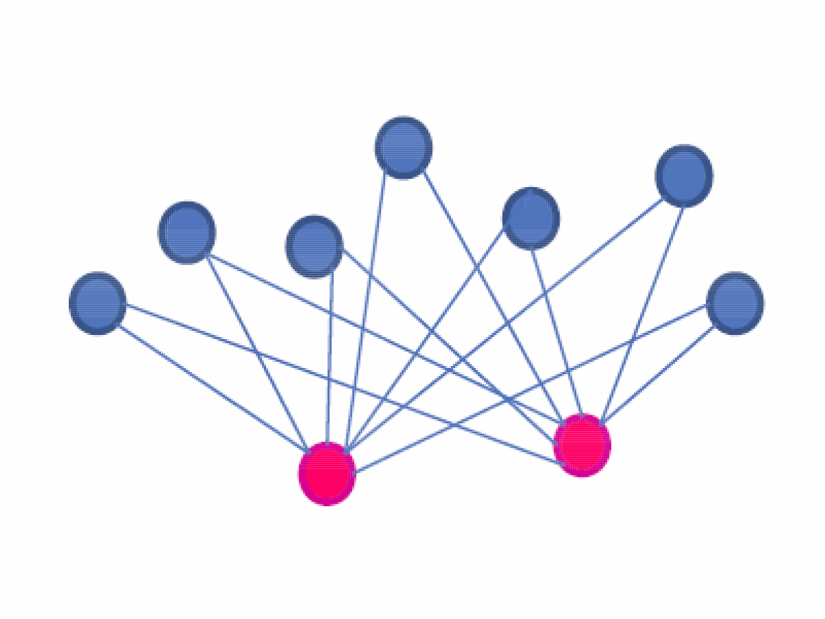
which vanishes for large system size. Green lines in Fig.5 show that the amount of entanglement generated between qubits initially in the ground state is negligible compared to that of qubits kk and jj. Therefore in the stationary state we have a bipartite graph as depicted in Fig.6.

Refer to caption
Figure 6: Pictorial representation of the leading stationary correlations (edges) among qubits (circles). Red (reps. blue) circles represents qubits initially in the excited (resp. ground) state.

V Concluding Remarks

In conclusion, we have studied the entanglement dynamics of a system composed of an arbitrary number of qubits dissipating into a common environment.

The consideration of models like this is becoming increasingly pressing with the continuing miniaturization of information processing devices. For instance, in solid state implementations qubits may be so closely spaced that they can experience the same environment [9].

By considering initial states whose evolution is confined on low dimensional subspaces of the operators space we found that pairwise entanglement is not created at any time between initially excited qubits. Instead, it is created and persists at steady state for pairs of initially excited and initially not excited qubits. The same holds true for pairs of qubits initially in the ground state, but in such a case the amount of entanglement is negligibly smaller than the previous case. This lead to the emergence of structures (subgraphs) which makes this subject appealing also from the perspective of complex networks [10].

Finally, it is worth noticing that the extension of the presented analysis to states with an arbitrary number ee of initial excitations can be done in a computationally efficient way due to the polynomial scaling of d​i​m​ℍρ⁡(0)dim\mathbb{H}_{\rho(0)} vs ee. We can arrive at such a scaling (much tighter with respect to the bound given in Eq.(4)), by simply observing the results in Sec.III and IV. In fact, in Sec.III the density matrix can be written, in the vector basis {|G⟩,|k⟩,|Ek̸⟩}\{|G\rangle,|k\rangle,|E_{\not k}\rangle\}, as

ρ=(a0000a1a30a3a2).\displaystyle\rho=\left(\begin{array}[]{ccc}a_{0}&0&0\\ 0&a_{1}&a_{3}\\ 0&a_{3}&a_{2}\end{array}\right).

Furthermore, in Sec.IV the density matrix can be written, in the vector basis {|G⟩,|Ek̸,l̸⟩,|k+l⟩,|k,l⟩,|B⟩,|H⟩}\{|G\rangle,|E_{\not k,\not l}\rangle,|k+l\rangle,|k,l\rangle,|B\rangle,|H\rangle\}, as

ρ=(b0000000b1b30000b3b2000000b4b7b8000b7b5b9000b8b9b6).\displaystyle\rho=\left(\begin{array}[]{cccccc}b_{0}&0&0&0&0&0\\ 0&b_{1}&b_{3}&0&0&0\\ 0&b_{3}&b_{2}&0&0&0\\ 0&0&0&b_{4}&b_{7}&b_{8}\\ 0&0&0&b_{7}&b_{5}&b_{9}\\ 0&0&0&b_{8}&b_{9}&b_{6}\end{array}\right).

Then, given the diagonal block structure of the above matrices (V) and (V), we can argue that for a number of initially excitations ee the density matrix will have e+1e+1 blocks of dimensions 1,2,⋯,e+11,2,\cdots,e+1. Each block of dimension rr (with 1≤r≤e+11\leq r\leq e+1) has r⁡(r+1)2\frac{r(r+1)}{2} number of real parameters. Since the total number of parameters in the matrix determines the dimension of ℍρ⁡(0)\mathbb{H}_{\rho(0)}, we will have d​i​m​ℍρ⁡(0)=∑r=1e+1r⁡(r+1)2=(1+e)​(2+e)​(3+e)/6dim\mathbb{H}_{\rho(0)}=\sum_{r=1}^{e+1}\frac{r(r+1)}{2}=(1+e)(2+e)(3+e)/6 which is polynomial of degree 3 of ee.

Appendix A Solution of Eqs. (21) and (22)

b0\displaystyle b_{0} =\displaystyle= 8n−2​(e−4​(n−1)​t−14​(n−1)−e−2​n​t−12​n),\displaystyle\frac{8}{n-2}\left(\frac{e^{-4(n-1)t}-1}{4(n-1)}-\frac{e^{-2nt}-1}{2n}\right),
b1\displaystyle b_{1} =\displaystyle= 4(n−2)​n2​(1−e−n​t)2​(1−e−2​(n−2)​t),\displaystyle\frac{4}{(n-2)n^{2}}(1-e^{-nt})^{2}(1-e^{-2(n-2)t}),
b2\displaystyle b_{2} =\displaystyle= −(1−e−2​(n−2)​t)​(2​e−n​t+n−2)2(n−2)​n2,\displaystyle-\frac{(1-e^{-2(n-2)t})(2e^{-nt}+n-2)^{2}}{(n-2)n^{2}},
b3\displaystyle b_{3} =\displaystyle= 2​(1−e−n​t)​(1−e−2​(n−2)​t)​(n−2​(1−e−n​t))(n−2)​n2,\displaystyle\frac{2(1-e^{-nt})(1-e^{-2(n-2)t})(n-2(1-e^{-nt}))}{(n-2)n^{2}},
b4\displaystyle b_{4} =\displaystyle= (2​(n−1)​e−(n−2)​t+2​e−2​(n−1)​t+n⁡(n−3)n⁡(n−1))2,\displaystyle\left(\frac{2(n-1)e^{-(n-2)t}+2e^{-2(n-1)t}+n(n-3)}{n(n-1)}\right)^{2},
b5\displaystyle b_{5} =\displaystyle= 4​e−4​(n−1)​t(n−1)2​n2+4​(n−4)​e−(3​n−4)​tn2​(n−1)​(n−2)+(n−4)2​e−2​(n−2)​tn2​(n−2)2−4​(n−3)​e−2​(n−1)​tn​(n−1)2​(n−2)\displaystyle\frac{4e^{-4(n-1)t}}{(n-1)^{2}n^{2}}+\frac{4(n-4)e^{-(3n-4)t}}{n^{2}(n-1)(n-2)}+\frac{(n-4)^{2}e^{-2(n-2)t}}{n^{2}(n-2)^{2}}-\frac{4(n-3)e^{-2(n-1)t}}{n(n-1)^{2}(n-2)}
−2​(n−3)​(n−4)​e−(n−2)​tn⁡(n−1)​(n−2)2+((n−3)(n−1)​(n−2))2,\displaystyle-\frac{2(n-3)(n-4)e^{-(n-2)t}}{n(n-1)(n-2)^{2}}+\left(\frac{(n-3)}{(n-1)(n-2)}\right)^{2},
b6\displaystyle b_{6} =\displaystyle= 4​(e−2​(n−1)​tn⁡(n−1)−2​e−(n−2)​tn⁡(n−2)+1(n−1)​(n−2))2,\displaystyle 4\left(\frac{e^{-2(n-1)t}}{n(n-1)}-2\frac{e^{-(n-2)t}}{n(n-2)}+\frac{1}{(n-1)(n-2)}\right)^{2},
b7\displaystyle b_{7} =\displaystyle= 4​e−4​(n−1)​tn2​(n−1)2+2​(3​n−8)​e−(3​n−4)n2​(n−1)​(n−2)+2​(n−3)2​e−2​(n−1)​tn​(n−1)2​(n−2)+2​(n−4)​e−2​(n−2)​tn2​(n−2)\displaystyle 4\frac{e^{-4(n-1)t}}{n^{2}(n-1)^{2}}+2\frac{(3n-8)e^{-(3n-4)}}{n^{2}(n-1)(n-2)}+2\frac{(n-3)^{2}e^{-2(n-1)t}}{n(n-1)^{2}(n-2)}+2\frac{(n-4)e^{-2(n-2)t}}{n^{2}(n-2)}
+(n−3)​(n−6)​e−(n−2)​tn​(n−1)​(n−2)−(n−3)2(n−1)2​(n−2),\displaystyle+\frac{(n-3)(n-6)e^{-(n-2)t}}{n(n-1)(n-2)}-\frac{(n-3)^{2}}{(n-1)^{2}(n-2)},
b8\displaystyle b_{8} =\displaystyle= 4​(e−4​(n−1)​tn2​(n−1)2+(n−4)​e−(3​n−4)​tn2​(n−1)​(n−2)CLOSE\displaystyle 4\left(\frac{e^{-4(n-1)t}}{n^{2}(n-1)^{2}}+\frac{(n-4)e^{-(3n-4)t}}{n^{2}(n-1)(n-2)}\right.
OPEN+(n2−5​n+8)​e−2​(n−1)​t2​n​(n−1)2​(n−2)−2​e−2​(n−2)​tn2​(n−2)−(n−4)​e−(n−2)​tn​(n−1)​(n−2)+(n−3)2​(n−1)2​(n−2)),\displaystyle\left.+\frac{(n^{2}-5n+8)e^{-2(n-1)t}}{2n(n-1)^{2}(n-2)}-2\frac{e^{-2(n-2)t}}{n^{2}(n-2)}-\frac{(n-4)e^{-(n-2)t}}{n(n-1)(n-2)}+\frac{(n-3)}{2(n-1)^{2}(n-2)}\right),
b9\displaystyle b_{9} =\displaystyle= −2​(−2​e−4​(n−1)​tn2​(n−1)2−(n−8)​e−(3​n−4)​tn2​(n−1)​(n−2)CLOSE\displaystyle-2\left(-2\frac{e^{-4(n-1)t}}{n^{2}(n-1)^{2}}-\frac{(n-8)e^{-(3n-4)t}}{n^{2}(n-1)(n-2)}\right. (43)
OPEN+(n−5)​e−2​(n−1)​tn​(n−1)2​(n−2)+2​(n−4)​e−2​(n−2)​tn2​(n−2)2−(3​n−10)​e−(n−2)​tn⁡(n−1)​(n−2)2+(n−3)(n−1)2​(n−2)2).\displaystyle\left.+\frac{(n-5)e^{-2(n-1)t}}{n(n-1)^{2}(n-2)}+2\frac{(n-4)e^{-2(n-2)t}}{n^{2}(n-2)^{2}}-\frac{(3n-10)e^{-(n-2)t}}{n(n-1)(n-2)^{2}}+\frac{(n-3)}{(n-1)^{2}(n-2)^{2}}\right).

References

  • [1] R. Horodecki, P. Horodecki, M. Horodecki, K. Horodecki, Rev. Mod. Phys. 81, 865 (2009)
  • [2] M. B. Plenio and S. F. Huelga, Phys. Rev. Lett. 88, 197901 (2002); S. Clark, A. Peng, M. Gu and S. Parkins , Phys. Rev. Lett. 91, 177901 (2003); S. Mancini and J. Wang, Eur. Phys. J. D 32, 257 (2005); L. Hartmann, W. Dur, H.J. Briegel, Phys. Rev. A 74, 052304 (2006); D. Angelakis, S. Bose and S. Mancini, Europhys. Lett. 85, 20007 (2007).
  • [3] H. Krauter, C. A. Muschik, K. Jensen, W. Wasilewski, J. M. Petersen, J. I. Cirac, E. S. Polzik, Phys. Rev. Lett. 107, 080503 (2011).
  • [4] B. Ghosh, A. S. Majumdar and N. Nayak, Phys. Rev. A 74, 052315 (2006); L. Memarzadeh and S. Mancini, Phys. Rev. A 83, 042329 (2011); M. Rafiee, C. Lupo, H. Mokhtari and S. Mancini Phys. Rev. A 85, 042320 (2012): S. F. Huelga, A. Rivas and M. B. Plenio, Phys. Rev. Lett. 108, 160402 (2012).
  • [5] D. Braun, Phys. Rev. Lett. 89, 277901 (2002); F. Benatti, R. Floreanini and M. Piani, Phys. Rev. Lett. 91, 070402 (2003).
  • [6] H. P. Breuer and F. Petruccione, The Theory of Open Quantum Systems, Oxford University Press, Oxford (2002).
  • [7] H. Spohn, Rev. Mod. Phys. 52, 569 (1980).
  • [8] W.K. Wootters, Phys. Rev. Lett., 80, 2245 (1998).
  • [9] Y. Hu, Phys. Rev. A 75, 012314 (2007).
  • [10] R. Albert and A. L. Barabàsi, Rev. Mod. Phys. 74, 47 (2002); S. Perseguers, M. Lewenstein, A. Acín and J. I. Cirac, Nat. Phys. 6, 539 (2010).