An Iterative Action Minimizing Method for Computing Optimal Paths in Stochastic Dynamical Systems
Abstract
We present a numerical method for computing optimal transition pathways and transition rates in systems of stochastic differential equations (SDEs). In particular, we compute the most probable transition path of stochastic equations by minimizing the effective action in a corresponding deterministic Hamiltonian system. The numerical method presented here involves using an iterative scheme for solving a two-point boundary value problem for the Hamiltonian system. We validate our method by applying it to both continuous stochastic systems, such as nonlinear oscillators governed by the Duffing equation, and finite discrete systems, such as epidemic problems, which are governed by a set of master equations. Furthermore, we demonstrate that this method is capable of dealing with stochastic systems of delay differential equations.
1 Introduction
One important aspect of the study of dynamical systems is the study of noise on the underlying deterministic dynamics [1, 2]. Although one might expect the deterministic dynamics would be only slightly perturbed in the presence of small noise, there are now many examples where noise causes a dramatic measurable change in behavior, such as noise induced switching between attractors in continuous systems [3] , and noise induced extinction in finite size systems [2].
In systems transitioning between coexisting stable states, much research has been done primarily because switching can be now investigated for a large variety of well-controlled micro- and mesoscopic systems, such as trapped electrons and atoms, Josephson junctions, and nano- and micro-mechanical oscillators [4, 5, 6, 7, 8, 9, 10, 11, 12, 13]. In these systems, observed fluctuations are usually due to thermal or externally applied noise. However, as systems become smaller, an increasingly important role may be played also by non-Gaussian noise. It may come, for example, from one or a few two-state fluctuators hopping at random between the states, in which case the noise may be often described as a telegraph noise. It may also be induced by Poisson noise [14].
In finite size populations or systems, extinction occurs in discrete, finite populations undergoing stochastic effects due to random transitions or perturbations. The origins of stochasticity may be internal to the system or may arise from the external environment [15, 16], and in most cases is non-Gaussian [17, 18].
Extinction depends on the nature and strength of the noise [19], outbreak amplitude [20] and seasonal phase occurrence [21]. For large populations, the intensity of internal population noise is generally small. However, a rare, large fluctuation can occur with non-zero probability and the system may be able to reach the extinct state. Since the extinct state is absorbing due to effective stochastic forces, eventual extinction is guaranteed when there is no source of reintroduction [22, 23, 1].
Models of finite populations, which include extinction processes, are effectively described using the master equation formalism, and predict probabilities of rare events [17]. For many problems involving extinction in large populations, if the probability distribution of the population is quasi-stationary, the probability of extinction is a function that decreases exponentially with increasing population size. The exponent in this function scales as a deterministic quantity called the action [24]. It can be shown that a trajectory that brings the system to extinction is very likely to lie along a most probable path, called the optimal path. It is a major property that a deterministic quantity such as the action can predict the probability of extinction, which is inherently a stochastic process, and is also formulated in continuous systems driven by noise [25, 26].
Locating the optimal path is important since the quantity of interest, whether it is the switching or extinction rate, depends on the probability to traverse this path. Therefore, a stochastic control strategy based on the switching or extinction rates can be determined by its effect on the optimal path [26].
The optimal path formalism converts the entire stochastic problem to a mechanistic dynamical systems problem with definitive properties. First, the optimal path is a solution to a Hamiltonian dynamical system. In the case of continuous stochastic models, the dimension of the system is twice that of the original stochastic problem. The other dimensions are conjugate momenta, and typically represent the physical force of the noise which induces escape from a basin of attraction to either switch or go extinct. Finally, due to the symplectic structure of the resulting Hamiltonian system, it can be shown that both attractors and saddles of the original system become saddles of the Hamiltonian system.
One of the main obstacles to finding the optimal path is that it is an inherently unstable object. That is, if one one starts near the path described by the Hamiltonian system, then after a short time, the dynamics leaves the neighborhood of the path. In addition, although the path may be hyperbolic near the saddle points, it may not be hyperbolic along the rest of the path. Solving such problems using shooting methods for simple epidemic models [27, 28, 29], or mixed shooting using forward and backward iteration [30, 31] will in general be inadequate to handle even the simplest unstable paths in higher dimensions. Therefore, it is the goal of this paper to exemplify a robust numerical method to solve for the optimal path using a general accurate discrete formulation applied to the Hamiltonian two point boundary value problem.
The method we employ here to compute the optimal paths is similar to the generalized minimum action method (gMAM), [32] which is a blend of the string method [33] and minimum action method [34]. Both are iterative methods which globally minimize the action along the path. These other techniques differ from ours primarily in that our formulation of the problem allows a direct, fully explicit iterative scheme, while the gMAM, in particular, employs a semi-implicit scheme. The numerical scheme presented here should provide an easy to employ alternative to the methods discussed above for stochastic optimization problems which are formulated as Hamiltonian two-point boundary value problems.
The paper is organized as follows. We first briefly present the general SDE problem, and the formulation of the corresponding deterministic Hamiltonian system by treating the switching as a rare event. We then present the details of the numerical approximation technique we will use to find the path which maximize the probability of switching. Using this technique, we then demonstrate finding the optimal path from a stable focus to the unstable saddle for the unforced Duffing equation, then compute optimal extinction pathways for a simple epidemic model, and finally adapt our method to find optimal transition paths in stochastic delay differential systems.
2 General Problem
Consider a general stochastic differential equation of the form
| (1) |
where represents the physical quantity in state space and and the matrix 11 1 Throughout the paper, boldface lower-case letters will indicate vectors, while boldface upper-case letters will indicate matrices. is given by , where the ’s are general nonlinear functions. We suppose the noise is a vector having a Gaussian distribution with intensity , and independent components. It is characterized by its probability density functional ,
| (2) |
We wish to determine the path with the maximum probability of traveling from the initial state to the final state , where the initial and final states are equilibria of the noise-free (i.e. ) version of Eq. 1 given by . These states typically characterize a generic problem of study in stochastic systems, such as switching between attractors, escape from a basin of attraction, or extinction of population. We assume the noise intensity is sufficiently small so that in our analysis sample paths will limit on an optimal path as . We also remark that is formally the time derivative of a Brownian motion, sometimes referred to as white noise [35].
For sufficiently small, and examining the tail of the distribution for a large fluctuation (which is assumed to be a rare event), the probability of observing such a large fluctuation scales exponentially by [36, 37],
| (3) |
where,
| (4) |
where the Lagrange multipliers also correspond to the conjugate momenta of the equivalent Hamilton-Jacobi formulation of this problem.22 2 The vector multiplication here is assumed to be an inner product. The exponent of Eq. 3 is called the action, and corresponds to the minimizer of the action in the Hamilton-Jacobi formulation which occurs along the optimal path. This path will minimize the integral of Eq. 4, and is found by setting the variations along the path to zero.
The resulting equations of motion for the states and Lagrange multipliers are given by
| (5) | ||||
Here , where Einstein summation is assumed over repeated indices. Note that is invariant, and recovers the noise free case of Eq. 1. The above equations can be shown to satisfy the motion of a Hamiltonian system with Hamiltonian
| (6) |
That is, the dynamics of a given path satisfy and
In addition to solving the Hamiltonian system of dynamics, the full problem specification of an optimal path requires boundary conditions for both state and momenta . The boundary conditions of the optimal path consist of two steady states, and at equilibrium. Typically, the boundary conditions are derived from the equations of motion defined by Eq. 6. Since they are derived as steady state conditions, they are asymptotic boundary conditions that are infinite limits in the temporal line. In addition, since we have assumed the Hamiltonian is time-independent, energy is conserved, and the path must lie on a fixed energy surface. Notice, in the case where the Hamiltonian is time invariant, and given that the action is minimized along the optimal path, the Hamilton-Jacobi equations require a zero-energy constraint, i.e. . We now describe how to solve the Hamiltonian system as a two point boundary value problem on a restricted energy surface.
2.1 Stability of Steady State Solutions
As stated above, we seek the optimal path between two steady state solutions and where and are steady state solutions of the zero-noise case of Eq. 1, and thus satisfy . Depending upon the linear stability of the zero-noise steady states, the stochastic transition from to may or may not be a rare event. For example, if the stability matrix of the general SDE Eq. 1 has at least one eigenvalue with positive real part, then it is an unstable or saddle point in the stochastic equation. Further, if has eigenvalues with all negative real parts, then it is a stable focus, and the transition from to will be deterministic restricted to and therefore not a rare event. The rare event, in this case, would be a transition from to , meaning noise drives the system out of the stable focus and onto the unstable/saddle point.
It is worth noting that all steady state solutions of the Hamiltonian system 5 which correspond to the deterministic steady state solutions of Eq. 1, i.e. , are saddle points. It is easy to see why this is true in the case of additive noise, i.e. . We can classify the steady states of Eq. 5 by calculating the eigenvalues of its stability matrix
| (7) |
at the steady states. The eigenvalues of are given by,
| (8) |
If we assume , then . Thus, if is an eigenvalue of , the stability matrix of the SDE problem given by Eq. 1, then is an eigenvalue of with eigenvector . Similarly, if , then -, which implies that is an eigenvalue of with eigenvector . Since are eigenvalues of , we can conclude that every steady state solution of Eq. 5 has eigenvalues with both positive and negative real parts and, thus, is a saddle. Thus, every steady state solution whose linearization has non-zero real part of the general stochastic equation, Eq. 1 regardless of stability becomes a saddle point when the system is converted to a Hamiltonian system. That is, deterministic attractors and saddles map to saddles in the Hamiltonian formulation.
3 Numerical Scheme
Our numerical approach involves using a finite differences scheme to write the system of ODEs as a high dimensional algebraic system, to which we apply a modified Newton’s Method to minimize the residual error until a solution is reached (to within some desired tolerance). As before, assume the Hamiltonian system in admits two steady states, and .
Then we seek the optimal path on the zero-energy surface that connects to . In this formulation, one would expect such a path to exhibit several properties when parametrized along . First, we assume the path starts at at . Since this point is an equilibrium solution, we should expect that the solution stays very near this value, that is, there exists such that for , has a transition region from and finally stays near , the second steady state for, . Numerically, we will approximate the solution on the finite domain so that the value at ) is arbitrarily close to the steady solution.
We map the interval 33 3 For the simulations below, unless otherwise specified. Ideally, is picked large enough so that and . i.e. the steady states are obtained up to machine precision for double precision numbers. onto using the linear transformation , and drop the “bar” notation for readability. On this discrete time domain, we write the system of ODEs as a system of nonlinear algebraic equations using central differences.
The simplest method is to employ a finite step size and use a uniform time step subdividing into equal segments. In practice, however, the simple uniform step size is not always the best choice since the optimal path tends to stay very near the stable points throughout most of the domain, and sometimes makes a relatively sharp transition near the center of the domain. In this case, it is helpful to use a nonuniform grid to resolve the sharp transition region using a fine mesh, and to use a coarse mesh near the edges where the solution is mostly flat. Thus, for the nonuniform time step , yielding the time series and corresponding function values , the derivative is approximated by the operator ,
| (9) |
At this point, we can write the generic system of nonlinear algebraic equations:
| (10) |
and solve this system using a general Newton’s Method for nonlinear systems of equations. To properly apply Newton’s method here, let be the extended vector of dimension containing the j-th Newton iterate (recalling that are defined on the timeseries given by ). Then will represent the initial guess. Let be the function defined by Eq. 10 acting on . Then to find the zeros of we employ a Newton scheme. A new Newton iterate is given by solving the linear system , using any one of a variety of methods such as LU decomposition or the generalized minimal residual method (GMRES) with appropriate preconditioners. Throughout this paper we will use LU decomposition with partial pivots optimized for a sparse linear system. Here the Jacobian is computed approximately using a central difference scheme.
Formally, this method is second order with respect to . The initial guess for this algorithm is constructed by the knowledge that the optimal path spends most of its time near the stable equilibria, and has a brief but sometimes sharp transition between the two states. One choice that has worked in practice is using functions like , with (where the parameter adjusts the sharpness of the jump), which have horizontal asymptotes at the appropriate critical values. Usually, though not always, is set so that for , .
Note that the zero-energy surface constraint is not imposed. Rather, the initial guess will start out near (at ) and (at ) which lie asymptotically close to the zero energy surface, and thus the final solution will have to lie on this surface since such a solution is time invariant (i.e. ). At each iterate, both the residual error and the Hamiltonian are checked at each point, and both must reach a desired tolerance in the norm before the procedure is completed.
Once the optimal path is computed, the action (i.e. the exponent) along the optimal path may be obtained with a simple integral,
| (11) |
Exhaustive convergence tests on the residual error for a variety of test problems for both the uniform and non-uniform grids have demonstrated the second order convergence for this method. We have noted some dependency on the initial guess in terms of the overall speed of convergence (or divergence for a particularly bad guess). The method generally produces a unique solution (up to possibly a horizontal shift in the time series seen in a few examples, which does not affect the path integrals of interest). This method has been reliable for a wide parameter regime for each of the test problems, with the limitations to be discussed below on a case by case basis.
This method, which we will henceforth refer to as the Iterative Action Minimization Method (IAMM), has several distinct advantages over other methods, the foremost of which is straightforward scalability to higher dimensions. For very high dimensional problems, the systems will eventually become too large to treat easily with a single processor, but this algorithm has proven efficient for up to six dimensional problems with a single processor. Further, this method lends itself to infinite dimensional problems, such as time delay stochastic differential equations, as will be demonstrated below.
4 Noise Induced Transitions
We demonstrate the numerical techniques by examining several bistable dynamical systems. Using methods discussed above, we explicitly approximate the optimal path between the two states and then numerically integrate along the path directly to compute the action.
4.1 Switching in the Duffing Equation
One of the standard nonlinear dynamical systems which exhibits bi-stability is Duffing’s equation. This equation is used to model certain types of nonlinear damped oscillators, and here we consider the singularly perturbed and unforced version [38],
| (12) | ||||
Here and control the size and nonlinear response of the restoring force, while controls the friction or damping on the system. The terms and are uncorrelated white noise sources applied to the acceleration and velocity respectively. When the perturbation fast and slow manifolds can be identified, while gives the unconstrained case. Rescaling time , applying eq. 6, and following the methodology above, we can write the system in the following general form,
| (13) |
with corresponding equations of motion,
| (14) | ||||
We will restrict our focus to the additive white noise case, .
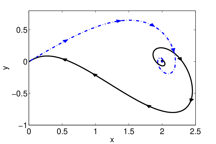
Note that the Hamiltonian system emits three known steady states and , all of which are saddle points. These steady states correspond to zero-noise critical points of Eq. 12, , a saddle point, and , the centers of the stable foci. The path from to can be found deterministically when , as any solution perturbed from the saddle node point will move along the solution curves and end up at either stable focus. A more interesting case is the optimal path from one of the focus points to the saddle-node point, which will require non-trivial momentum. Such momenta model the small noise effects which organize to force the trajectory across the basin of attraction, thus escaping from one attractor to the other.
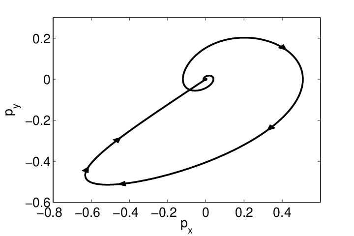
Figure 1 shows both the deterministic and optimal paths as computed using the IAMM developed above. For the deterministic path, the algorithm correctly predicts that the noise will be zero along this path, and that the action will be zero as the probability of going from to is one, and thus not a rare event. On the other hand, the path from to involves nontrivial action, and the effect of the noise along the optimal path is shown. This path lies on the zero-energy surface, and maximizes the probability of traveling from to for arbitrarily small noise intensities, . Figure 2 shows the residual error at each iterate used to generate the data for figure 1 until the convergence criteria is reached.


When , we can derive an analytical formulation for the action by using a center manifold analysis on Eq. 13 by following the work of [38]. Here the center manifold is given by , and we approximate it as,
| (15) |
By substituting equation 15 into equation 12 and equating like powers of , we arrive at a one dimensional form of equation 12 for the lowest order terms involving ,
| (16) |
Here the contribution of the uncorrelated noise terms are contained in a single noise source . The Hamiltonian form of 16 is,
| (17) |
We can find the nontrivial relationship ()between and on the zero energy surface directly, , and integrate along this path to predict the action along the optimal path. Since one may be interested in how the action scales relative to the distance between the two critical points we substitute the values and to better illustrate the scaling with respect to . Thus, with this substitution, we seek the action from to . From equation 11, this is a simple integral,
| (18) |
Thus, we can predict, for example, that the action from to should scale like the square of near the center manifold. Indeed, varying the parameter for the four-dimensional system, Eq. 14, predicts the same order scaling as seen below in Fig. 3. We also consider the scaling with respect to the damping parameter , and again, near the center manifold, the predictions are born out by integrating along the optimal path. Indeed, the scaling for the action predicted from the lowest order terms in the center manifold analysis seems to persist in the two-dimensional model.


Since it is not clear if the same relationship will work further away from the center manifold, we check the scaling with respect to and when in Eq.14 in figure 4. Interestingly, the leading order scaling of the action with respect to is still , just as it was near the center manifold. Meanwhile, the scaling with respect to is markedly different. Thus, we can predict both near and away from the center manifold how the action will scale as a function of the distance between the two equilibrium points.
4.2 SIS Epidemic Models
Next we consider a simple susceptible-infected-susceptible (SIS) epidemic model in the general noise case, as considered by [25]. This model is defined by a master equation which describes the probability of fluctuations between a susceptible or infected category in a population of individuals. Assuming is sufficiently large, we can write a mean field system of equations for the change of the population fractions of susceptible and infected individuals, denoted and respectively,
| (19) | ||||
For simplicity, the population in the mean field is assumed constant, i.e. births and deaths are equal. Here is the natural birth and death rate of both the susceptible and infected populations, is the contact rate, and is the natural recovery rate of the infected population.
Since we have assumed the population fraction of susceptible and infected individuals are conserved, we have . Under this constraint, assuming a small random fluctuation of only the infected individuals, we can use a methodology similar to the one described above (and worked out in detail in [25]) to write a Hamiltonian system,
| (20) |
We shall refer to equation 20 as the 1D SIS model equation. The optimal path will extend from the endemic state at to the extinct state , where . Using the methods introduced above, the optimal path (at typical parameter values) is given below. Integrating the momentum along this path gives the action, which is proportional to the probability of extinction. In this simple 1D SIS model, the predicted action scaling as a function of is given by solving the Hamiltonian directly for and solving the integral 11
Since this is one of the rare cases the optimal path can be found analytically, it is a great test case for our method. A comparison of the analytical action to the numerical action is shown in figure 5.

In the case of an SIS epidemic model with independent fluctuations on both the susceptible () and infected () populations, the Hamiltonian form of the equations is given by,
| (21) |
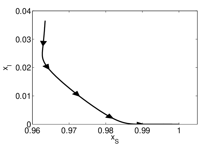
and we refer to this form as the 2D SIS model. The two states of interest for this system are the endemic state, and the nontrivial extinct state, . Using the procedure discussed above, we compute the optimal path from the endemic to the extinct state, and show a typical result in figure 6.

Instead of comparing the action scaling predicted here to an analytical formulation, we instead compare it to a Monte-Carlo simulation of the master equation for the initial system with a fixed population size of 20,000 individuals. In the Monte-Carlo simulation, a Gillespie algorithm is employed on the SIS model, and from all the simulations, a probability of extinction is computed for several values of . From these, a mean extinction time is derived, and the log of this mean extinction time should scale like the action predicted from the action integrals, from Eq. 11, computed using our approach. Figure 7 shows a comparison of the two approaches, and good agreement is seen between these two independent methods.

4.3 Finite Time Lyapunov Exponents
As demonstrated in [17], the optimal path to extinction coincides with ridges, i.e. maximal values, of the finite time Lyapunov exponents (FTLEs). Forgoston and others propose finding FTLE ridges as a method of computing optimal paths [17, 18, 39]. Here, we demonstrate that our approximation to the optimal path does indeed locally maximize the FTLE.
We proceed by using the methods outlined in [40, 41, 42, 43] to approximate the FTLEs at points on our optimal path, and at nearby points transverse to the optimal path. We begin by picking a point on the optimal path (generated by our method), and on nearby points some small distance away from the path.
For the given vector field, we assume we have a flow passing through initial point , , such that . The local linear variation at is defined by .
Using a fourth order Runge-Kutta method, we can integrate all the initial points , , forward in time over a fixed interval, and compute the finite time deformation rate of the local coordinates (i.e. Right Cauchy-Green Tensor) . The maximal eigenvalue of will give the FTLE .
Consider the case of the 1D SIS extinction model from above. Here, we will use a path computed above and compare the values near this path to the local FTLEs. In Figure 8a we plot the FTLEs over a square domain, and show that a local maximum (ridge) is attained precisely where the computed optimal path predicts.
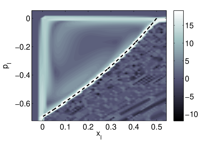

In higher dimensions, the maximal Lyapunov exponent is still exhibited along the optimal path [17]. For the 2D SIS model, note that the optimal path exists in four dimensions. Thus, the transverse direction is the set of points obtained by rotating a normal vector to the path around two Euler angles (which forms a 3D sphere for a given radius ). To illustrate FTLEs in this higher dimension framework, we must consider the “shell” around the initial starting point (and orthogonal to the path) at a fixed radius, and then compute FTLEs on this shell all along the optimal path. We expect that the maximal FTLE will occur along the optimal path, relative to nearby points on the transverse sphere. To illustrate this, we define as a unit vector orthogonal to the tangent vector of the optimal path at a given time, i.e. , and then examine the FTLE as a function of the two Euler angles for a given . Figure 8b shows just one cross section (over a short time interval), obtained by setting both rotation angles to either or the anitipodal angle , of this high dimensional object, as a function of , and demonstrates that the maximal FTLE is, indeed, along the optimal path.
5 Time Delayed SDEs
One advantage of the IAMM is that it allows the solution of stochastic delay-differential equations of the form,
| (22) |
Schwartz et. al [44] have demonstrated that the methodology introduced in section 2 can be adapted to write this system as a Hamiltonian system,
| (23) |
where . The equations of motion are given by,
| (24) | ||||
Note the appearance of both delay and advance terms in 24. Because of the appearance of the delay term, the Hamiltonian is no longer time invariant, and unlike in the previous examples, where , the zero-energy condition is not conserved.
We shall consider a one dimensional test case where , where the steady states are given by and , for . Again, we will assume additive noise , and derive the Hamiltonian system,
| (25) |
and the corresponding equations of motion,
| (26) | ||||
The IAMM needs only a few minor adjustments to compute these paths numerically. Primarily, the presence of the delay and advance terms will add additional entries into our linear system Eq. 10. Our method uses a non-uniform timestep, and so may not coincide exactly with one of our points at time . To overcome this, we can use Lagrange interpolation on the closest four points such that . Since we keep the time domain fixed the needed for each can be easily computed before the iterative scheme is started, and fewer or more terms can be used in the Lagrange interpolation scheme depending upon desired accuracy. Further, if or , i.e. the delay or advance terms fall outside of our numerical domain, then we can set or respectively.
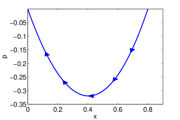
To demonstrate the effectiveness of the IAMM in solving these stochastic delay problems, we show sample paths in figure 9 and compare the scaling of the action versus a Monte-Carlo simulation of the stochastic delay difference equation in figure 10, and note the good agreement.

6 Discussion
We have considered the problem of finding the trajectory in stochastic dynamical systems that optimizes the probability of switching between two states, or causes one or more components to go extinct. In computing such a trajectory, called the optimal path, we needed to consider a numerical technique which could solve a Hamiltonian system with asymptotic boundary conditions in time. We have developed a numerical method, which we call the iterative action minimizing method (IAMM), for finding the optimal path of transition between two steady states in stochastic dynamical systems. This method is ideal for systems which can be written as two-point boundary value problems governed by Hamiltonian systems. We have validated the IAMM by presenting a variety of problems of interest, and have compared the numerical results with either analytic results or Monte-Carlo simulations of full stochastic systems.
As demonstrated here, the IAMM method is robust enough to be applicable to a variety of different types of problems, including continuous SDE systems, such as the Duffing equation, discrete epidemic models of finite population size, such as the SIS model, and stochastic delay differential equations, in which the deterministic problem is infinite dimensional. The methodology is straightforward enough to generalize to higher dimensions, in contrast to other commonly used methods, such as the shooting method, which is a major advantage of the IAMM.
The primary limitations of this method are scaling issues in very high state space dimensions, and the finesse required in picking an initial guess that guarantees convergence, both of which are typical of iterative methods of quasi-Newton type. In the limit of small noise or large system size, however, due to the robustness and ease of generalization to complex and high dimensional dynamical systems, the method offers a considerable advantage over simulating large systems, or systems which require many Monte Carlo runs to generate statistics of the transitions paths. As a result, we expect this method will be useful in efficiently solving a large variety of optimal transition problems in the field of stochastic dynamical systems.
7 Acknowledgments
The authors gratefully acknowledge the Office of Naval Research for their support under N0001412WX20083, and support of the NRL Base Research Program N0001412WX30002. Brandon Lindley is currently an NRC Postdoctoral Fellow. We thank Lora Billings for providing the Monte Carlo data used in figures 7 and 10, and Eric Forgoston for a preliminary reading of this manuscript.
References
- [1] C. W. Gardiner, Handbook of Stochastic Methods for Physics, Chemistry and the Natural Sciences, Springer-Verlag, 2004.
- [2] N. G. Van Kampen, Stochastic Processes in Physics and Chemistry, Elsevier, 2007.
- [3] M. I. Freidlin, A. D. Wentzell, Random Perturbations of Dynamical Systems, Springer-Verlag, 1984.
- [4] L. J. Lapidus, D. Enzer, G. Gabrielse, Stochastic phase switching of a parametrically driven electron in a penning trap, Phys. Rev. Lett. 83 (1999) 899–902.
- [5] I. Siddiqi, R. Vijay, F. Pierre, C. M. Wilson, L. Frunzio, M. Metcalfe, C. Rigetti, R. J. Schoelkopf, M. H. Devoret, D. Vion, D. Esteve, Direct observation of dynamical bifurcation between two driven oscillation states of a josephson junction, Phys. Rev. Lett. 94 (2005) 027005.
- [6] J. S. Aldridge, A. N. Cleland, Noise-enabled precision measurements of a duffing nanomechanical resonator, Phys. Rev. Lett. 94 (2005) 156403.
- [7] K. Kim, M. S. Heo, K. H. Lee, H. J. Ha, K. Jang, H. R. Noh, W. Jhe, Noise-induced transition of atoms between dynamic phase-space attractors in a parametrically excited atomic trap, Phys. Rev. A 72 (2005) 053402.
- [8] R. Gommers, P. Douglas, S. Bergamini, M. Goonasekera, P. H. Jones, F. Renzoni, Resonant activation in a nonadiabatically driven optical lattice, Phys. Rev. Lett. 94 (2005) 143001.
- [9] C. Stambaugh, H. B. Chan, Noise activated switching in a driven, nonlinear micromechanical oscillator, Phys. Rev. B 73 (2006) 172302.
- [10] B. Abdo, E. Segev, O. Shtempluck, E. Buks, Escape rate of metastable states in a driven nbn superconducting microwave resonator, J. Appl. Phys. 101 (2007) 083909.
- [11] A. Lupaşcu, S. Saito, T. Picot, P. C. De Groot, C. J. P. M. Harmans, J. E. Mooij, Quantum non-demolition measurement of a superconducting two-level system, Nature Physics 3 (2007) 119–123.
- [12] I. Katz, A. Retzker, R. Straub, R. Lifshitz, Signatures for a classical to quantum transition of a driven nonlinear nanomechanical resonator, Phys. Rev. Lett. 99 (2007) 040404–4.
- [13] I. Serban, F. K. Wilhelm, Dynamical tunneling in macroscopic systems, Phys. Rev. Lett. 99 (2007) 137001.
- [14] L. Billings, I. Schwartz, M. McCrary, A. Korotkov, M. Dykman, Switching exponent scaling near bifurcation points for non-gaussian noise, Physical review letters 104 (2010) 140601.
- [15] F. de Castro, B. Bolker, Mechanisms of disease-induced extinction, Ecol. Lett. 8 (2005) 117–126.
- [16] A. L. Lloyd, J. Zhang, A. M. Root, Stochasticity and heterogeneity in host-vector models, J. R. Soc. Interface 4 (2007) 851–863.
- [17] I. Schwartz, E. Forgoston, S. Bianco, L. Shaw, Converging towards the optimal path to extinction, Journal of The Royal Society Interface 8 (2011) 1699–1707.
- [18] E. Forgoston, S. Bianco, L. B. Shaw, I. B. Schwartz, Maximal sensitive dependence and the optimal path to epidemic extinction, Bull. Math. Bio. 73 (2011) 495–514.
- [19] B. A. Melbourne, A. Hastings, Extinction risk depends strongly on factors contributing to stochasticity, Nature 454 (2008) 100–103.
- [20] D. Alonso, A. J. McKane, M. Pascual, Stochastic amplification in epidemics, J. R. Soc. Interface 4 (2006) 575–582.
- [21] L. Stone, R. Olinky, A. Huppert, Seasonal dynamics of recurrent epidemics, Nature 446 (2007) 533–536.
- [22] M. S. Bartlett, Some evolutionary stochastic processes, J. Roy. Stat. Soc. B Met. 11 (1949) 211–229.
- [23] L. J. S. Allen, A. M. Burgin, Comparison of deterministic and stochastic SIS and SIR models in discrete time, Math. Biosci. 163 (2000) 1–33.
- [24] R. Kubo, K. Matsuo, K. Kitahara, Fluctuation and relaxation of macrovariables, J. Stat. Phys. 9 (1973) 51–96.
- [25] I. B. Schwartz, L. Billings, M. Dykman, A. Landsman, Predicting extinction rates in stochastic epidemic models, J. Stat. Mech.-Theory E. (2009) P01005.
- [26] M. I. Dykman, I. B. Schwartz, A. S. Landsman, Disease extinction in the presence of random vaccination, Phys. Rev. Lett. 101 (2008) 078101.
- [27] H. Keller, Keller, Numerical methods for two-point boundary-value problems, Dover Publications, 1992.
- [28] A. Kamenev, B. Meerson, Extinction of an infectious disease: A large fluctuation in a nonequilibrium system, Phys. Rev. E 77 (2008) 061107.
- [29] O. Gottesman, B. Meerson, Multiple extinction routes in stochastic population models, Phys. Rev. E 85 (2012) 021140.
- [30] V. Elgart, A. Kamenev, Rare event statistics in reaction-diffusion systems, Phys. Rev. E 70 (2004) 041106.
- [31] A. I. Chernykh, M. G. Stepanov, Large negative velocity gradients in burgers turbulence, Phys. Rev. E 64 (2001) 026306.
- [32] M. Heymann, E. Vanden-Eijnden, The geometric minimum action method: A least action principle on the space of curves, Comm. on Pure and Appl. Math. 61 (2008) 1052–1117.
- [33] E. Weinan, R. Weiqing, E. Vanden-Eijnden, String method for the study of rare events, Phys. Rev. B. 66 (2002) 052301.
- [34] E. Weinan, R. Weiqing, E. Vanden-Eijnden, Minimum action method for the study of rare events, Comm. on Pure and Appl. Math. 57 (2004) 0001–0020.
- [35] W. H. Fleming, Deterministic and Stochastic Optimal Control, Springer-Verlag, 1975.
- [36] M. I. Freidlin, A. D. Wentzell, Random Perturbations of Dynamical Systems, Springer-Verlag, New York, 2nd edition, 1998.
- [37] M. I. Dykman, Large fluctuations and fluctuational transitions in systems driven by colored gaussian-noise: a high-frequency noise, Phys. Rev. A 42 (1990) 2020–2029.
- [38] E. Forgoston, I. B. Schwartz, Escape rates in a stochastic environment with multiple scales, SIAM J. Appl. Dyn. Syst. 8 (2009) 1190–1217.
- [39] A. Kessler, L. B. Shaw, I. B. Schwartz, On the construction of optimal paths to extinction, U.S. naval Research Laboratory Report No. 6790-12-9374 (2012).
- [40] G. Haller, Finding finite-time invariant manifolds in two-dimensional velocity fields, Chaos 10 (2000) 99–108.
- [41] G. Haller, Distinguished material surfaces and coherent structures in three-dimensional fluid flows, Physica D 149 (2001) 248–277.
- [42] G. Haller, Lagrangian coherent structures from approximate velocity data, Phys. Fluids 14 (2002) 1851–1861.
- [43] S. C. Shadden, F. Lekien, J. E. Marsden, Definition and properties of Lagrangian coherent structures from finite-time Lyapunov exponents in two-dimensional aperiodic flows, Physica D 212 (2005) 271–304.
- [44] I. B. Schwartz, T. Carr, L. Billings, M. Dykman, Noise Induced Switching in Delayed Systems, arXiv:1207.7278v1 (2012).