Distributed and Autonomous Resource and Power Allocation for Wireless Networks
Abstract
In this paper, a distributed and autonomous technique for resource and power allocation in ofdma (ofdma) femto-cellular networks is presented. Here, rb and their corresponding transmit powers are assigned to the user(s) in each cell individually without explicit coordination between fbs. The “allocatability” of each resource is determined utilising only locally available information of the following quantities:
- •
the required rate of the user;
- •
the quality (i.e., strength) of the desired signal;
- •
the level of interference incident on each rb; and
- •
the frequency-selective fading on each rb.
Using a fuzzy logic system, the time-averaged values of each of these inputs are combined to determine which rb are most suitable to be allocated in a particular cell, i.e., which resources can be assigned such that the user requested rate(s) in that cell are satisfied. Furthermore, la (la) is included, enabling users to adjust to varying channel conditions. A comprehensive study in a femto-cell environment is performed, yielding system performance improvements in terms of throughput, energy efficiency and coverage over state-of-the-art icic (icic) techniques.
Index Terms:
autonomous resource allocation, distributed icic, fuzzy logic, ofdma, femto-cellular networks.I Introduction
Future wireless networks are moving towards heterogeneous architectures, where in each cell a user may have over four different types of ap (e.g., macro-, pico-, femto-cells, relays and/or remote radio heads) [1]. Intuitively, this has many positive effects for a ms (ms), which can now choose from several bs to find the most suitable. However, pico- and femto-cellular overlays also imbue many difficulties, e.g., cell-organisation/optimisation, resource assignment to users, and especially interference coordination between ap within the same and neighbouring cells. Standard icic techniques based on network architectures [2, 3] only go so far in dealing with these challenges, and hence a new approach is necessary.
I-A Challenges in hetnet
Through the various types, locations and dense deployment of ap, and the different transmissions powers/ranges associated with them, numerous technical challenges are posed by femto/pico-cell overlays [1, 4, 5]. These mainly fall into the following areas:
- •
Network self-organisation - Self-configuration and -optimisation are required of all cells. In cellular networks, such organisation can be performed via optimisation techniques [6], however these tasks become increasingly difficult given the additional ap and network parameters to be considered, motivating a distributed configuration approach [7].
- •
- •
Interference - Cross-tier interference created to/from the overlaid cells (e.g., pico-/femto-cells) must be mitigated to maintain performance, especially if access to these cells is restricted. High intra-femto-tier interference due to dense deployment is also of concern. The handling of this interference is paramount to the performance of such future networks, of which the main sources in densely deployed femto-cell scenarios [1] can be given as
- –
Unplanned deployment- Low-power nodes such as femto-cells are deployed by end-users at “random” locations, and can be active or inactive at any time, further randomising their interference. Continuous sensing and monitoring is required by cells to dynamically/adaptively mitigate interference from the other tiers [8].
- –
Closed-subscriber access - Restricted access control of pico- and femto-cells may lead to strong interference scenarios in downlink and uplink if users cannot handover.
- –
Node transmission power differences - The lower power of nodes such as pico- and femto-cells can cause associations downlink/uplink interference problems.
- –
In general, these issues motivate the need for decentralised, autonomous interference coordination schemes that operate independently on each cell, utilising only local information, yet achieving efficient/near-optimal solutions for the network. By allowing bs (all types) and ms to individually optimise their resource allocations and transmission powers, a global optimum may be found without centralised algorithms governing the system. This would substantially reduce not only the amount of signalling but also the operation complexity of the network.
I-B Randomly and Densely Deployed Femto-cells
Here, we address the relatively unexplored topic of icic for randomly deployed femto-cells. Due to the relative modernity of the femto-cell concept, and the innate random deployment of femto-cells within a macro-cell, most interference coordination techniques are utilised for interference reduction to the macro-cell, rather than interference protection between femto-cells.
The state-of-the-art interference coordination for lte hetnet is the abs (abs): a time-domain icic technique where an aggressor bs creates “protected” subframes for a victim bs by reducing its transmission activity on these [9]; the occurrences of the abs are known a priori at the coordinating bs. Thus, throughput improvements are induced via the provided interference protection [10]. However, the omitted transmission frames may have adverse affects on the data rates at the agressor bs. Furthermore, without guaranteed backhaul connections, fbs may not be able coordinate the abs slots. In this paper, we provide resource and power allocation for femto-femto interference environments which requires no signalling between fbs, and enhances the overall throughput, energy efficiency and fairness of the femto-network.
On another note, recent research has seen the emergence of autonomous coordination techniques for son [11, 12], where transmit powers on subbands is adjusted independently in each cell via local and network utility optimisation. These utilities are based on the average rate in the cell, however do not consider user-specific resource allocation for additional interference coordination. Furthermore, the proposed strategies do not consider heterogeneous architectures that will inevitably describe future networks. Finally, the suggested algorithms assume still some signalling between neighbouring bs, hence cannot be considered fully autonomous, and may also limit their applicability specifically for femto-cell networks.
Finally, the application of fuzzy logic in collaboration with reinforcement learning techniques is comprehensively studied in [13], in order to tune the outputs of fuzzy inference systems. The application to wireless network coordination is investigated in [14, 15, 16], where fuzzy logic reduces the complexity of the learning algorithms by providing coarse evaluations of the network state. On a cell-individual basis, by again adapting subband transmission powers [14], modifying the downlink rntp (rntp) thresholds [15], or adjusting the antenna downtilt [16] the interference on specific resources can be controlled or removed completely, respectively. On the other hand, QoS requirements of individual users are neglected, a perspective that we attempt to address here. In addition, we employ a holistic approach by considering many key parameters to perform resource allocation (i.e., frequency reuse) and power control in all cells individually.
In this paper, we introduce a novel, low-complexity, distributed and autonomous icic technique, that performs independent resource and power allocation in each cell, eliminating explicit signalling between fbs. The rest of the paper is structured as follows: Section II describes the system deployment scenario and channel environment, Section III explains the fuzzy logic icic protocol and its performance in femto-cellular networks is analysed in Section IV. In Section V the simulation is described, and Section VI portrays and discusses the simulation results. Finally, some concluding remarks are offered in Section VII.
II System and Channel Model
An ofdma network is considered, where the system bandwidth is divided into rb. A rb defines one basic time-frequency unit of bandwidth . All ms can transmit up to a fixed maximum power . Perfect time and frequency synchronisation is assumed.
Universal frequency reuse is considered, such that each femto-cell utilises the entire system bandwidth . The set of rb , where , is distributed by each bs to its associated ms(s). Throughout this paper, is used to define any ms, and the bs with which this ms is associated. The received signal observed by msu from bs on rb is given by
| (1) |
where signifies the channel gain between the msu and its serving bs, observed on rb . Furthermore, denotes the transmit power of msu on rb , the desired received signal, the thermal noise, and the co-channel interference received on rb from ms in neighbouring cells. The interference is defined by
| (2) |
where represents the set of interferers (i.e., set of ms in neighbouring cells that are also assigned rb ). Hence, the sinr (sinr) observed at the msu on rb is calculated by
| (3) |
Following this, the user throughput is calculated as the data transmitted on the assigned rb that have achieved their sinr target
| (4) |
where is the number of rb assigned to msu achieving , is the total number of rb allocated to msu, is the indicator function, the number of subcarriers per rb, the symbol rate per subcarrier, and the mcs (mcs) given in Table I11 1 In Table I, the modulation and coding orders are taken from lte [17], and the sinr ranges from [18]. In general, these values are operator specific, and hence are not standardised..
| CQI | min. | Code | Efficiency | |
|---|---|---|---|---|
| index | SINR [dB] | Modulation | rate | [bits/sym] |
| 0 | - | None | - | 0 |
| 1 | -6 | QPSK | 0.076 | 0.1523 |
| 2 | -5 | QPSK | 0.12 | 0.2344 |
| 3 | -3 | QPSK | 0.19 | 0.3770 |
| 4 | -1 | QPSK | 0.3 | 0.6016 |
| 5 | 1 | QPSK | 0.44 | 0.8770 |
| 6 | 3 | QPSK | 0.59 | 1.1758 |
| 7 | 5 | 16QAM | 0.37 | 1.4766 |
| 8 | 8 | 16QAM | 0.48 | 1.9141 |
| 9 | 9 | 16QAM | 0.6 | 2.4063 |
| 10 | 11 | 64QAM | 0.45 | 2.7305 |
| 11 | 12 | 64QAM | 0.55 | 3.3223 |
| 12 | 14 | 64QAM | 0.65 | 3.9023 |
| 13 | 16 | 64QAM | 0.75 | 4.5234 |
| 14 | 18 | 64QAM | 0.85 | 5.1152 |
| 15 | 20 | 64QAM | 0.93 | 5.5547 |
Finally, the system capacity is calculated as the sum throughput of all ms in the network
| (5) |
The power efficiency measures the data rate per unit of transmit power (or, alternatively, the data sent per unit of energy) of msu. This is defined as follows:
| (6) |
where is the transmit power of msu, and the achievable capacity from (4). The availability is defined as the proportion of ms that have acquired their desired rate, i.e.,
| (7) |
where is a random variable denoting the number of ms in the scenario and is the desired rate of msu. Lastly, Jain’s Fairness Index [19] is used to calculate the throughput fairness of the system in each time slot
| (8) |
where the vector denotes the achieved throughputs of all ms in the system.
II-A Scenario Construction
A apartment grid is considered for the femto-cell scenario, where the probability describes the likelihood of an active fbs in a given apartment. Furthermore, we assume that multiple ms may be present in an apartment. As it is unlikely all cells will have the same number of ms, the user generation is implemented via probability table, where depending on the maximum number of users allowed per cell, the number of ms present in cell is randomly chosen. Table II gives two examples of probability tables, where a) equal probabilities are given to all , or b) the probability reduces with each additional ms.
| 1 | 2 | 3 | 4 | |
|---|---|---|---|---|
| 1 | ||||
| 0 | ||||
| 0 | 0 | |||
| 0 | 0 | 0 |
or 1 2 3 4 1 0 0 0 0 0 0
Here, we utilise . An example of such a scenario is shown in Fig. 1. In each active femto-cell, both the ms and fbs are uniformly distributed in the apartment. Due to the private deployment of femto-cells a closed-access system is assumed [20], so each ms is assigned to the fbs in its apartment, even if a foreign cell exhibits superior link conditions.

II-B Channel Model
In general, the channel gain, , between a transmitter and receiver , observed on rb and separated by a distance is determined by the path loss, log-normal shadowing, and channel variations caused by frequency-selective fading:
| (9) |
where describes the channel transfer function between transmitter and receiver on rb , is the distance-dependent path loss (in dB) and is the log-normal shadowing value (in dB) with standard deviation , as described in [21]. The channel response generally exhibits time and frequency dispersions, however channel fluctuations within a rb are not considered as the rb dimensions are significantly smaller than the coherence time and bandwidth of the channel [22]. Furthermore, the path loss is identical on all rb assigned to the ms. Finally, the delay profiles used to generate the frequency-selective fading channel transfer factor are taken from applicable propagation scenarios in [21], [23].
The path loss model used to calculate is for indoor links [24], i.e., the link (desired or interfering) between a fbs and an indoor ms, and calculates the path loss as
| (10) |
where is the distance between transmitter and receiver, and are the channel parameters.
III Distributed and Autonomous Resource Allocation
Due to the customer-side random deployment of femto-cells, and the resulting lack of fixed connective infrastructure, fbs must perform resource and power allocation utilising locally available information only. To maximise the performance in its own cell, a fbs must attempt to allocate rb such that the desired signal on these is maximised, while the interference incident from neighbouring cells is minimal. Furthermore, the bs must allocate enough resources such that the rate requirements of the user(s) in the cell are fulfilled. The necessary, and locally available, information is therefore clearly determined:
- •
the required rate of a user determines the number of rb that need to be assigned;
- •
the quality (i.e., strength) of the desired signal dictates the necessary transmit power;
- •
the level of interference incident on the rb strongly influences their allocatability; and
- •
the frequency-selective fading profile also affects the preferable rb to be allocated.
All of these variables are locally available at the fbs in the reverse link, and at the ms(s) in the forward link, necessitating no extra information to be exchanged between bs.
III-A Fuzzy Logic for Autonomous Interference Coordination
In general, the resource and power allocation problem for a multi-cellular wireless network belongs to the class of minlp (minlp) problems; obtaining the solutions to these is known to be -hard [25, 26]. Therefore, it is clear that a heuristic for local, autonomous resource management is required to solve this problem. A machine learning approach where fbs acquire information about their transmission conditions over time would be such a viable solution, however can prove complex without the availability of training data. Therefore, we introduce fuzzy logic as our heuristic, through which “expert knowledge” is incorporated in the rb allocation decision process.
The decision system, in its most simplified form, is represented in Fig. 2. In broad terms, the system evaluates which rb(s) are most suitable to be allocated to the ms in a particular time slot, and determines the transmit power on these rb to generate the required sinr such that the user’s rate can be met. Obviously, an rb receiving little or no interference situated in a fading peak is most suitable for allocation to the femto-user, whereas any rb(s) receiving high interference, or experiencing deep fades, are much less appropriate.

In fuzzy logic, an input range is divided into multiple “membership functions” which give a coarse evaluation of the variable. By combining the membership values of the inputs through various rules, the allocatability of each rb is determined. The output is also “fuzzy,” indicating how suitable (or unsuitable) an rb is given the current inputs, avoiding a hard yes/no decision.
In each time slot, the fbs allocates the most applicable rb to each ms, and data transmission is performed. Based on the received signal levels from the desired user and interfering ms, the bs updates its information to more accurately represent the long-term interference and fading environments of its cell. This updated information is utilised in the next time slot to again carry out the, hopefully improved, resource and power allocation. The same operation is performed in all femto-cells in the scenario, and the rb allocations are continuously individually optimised until the system converges to a stable solution, in which the user(s) in each cell are satisfied.
III-A1 Inputs
The input variables considered in the fuzzy logic system are:
- •
The required rate of the ms is defined by the service being demanded by the user. Here, the values “Low,” “Low-medium,” “Medium-high,” and “High” are used to categorise the rate requested by the user. The ranges of these are dependent on the user scenario (e.g., in femto-cells, a higher rate can be requested due to the superior channel conditions). This is a per-user requirement, and thus is equivalent for all rb.
- •
The desired signal level describes the transmission conditions from transmitter to receiver, i.e., the stronger the desired signal, the better the channel between the two. The signal power domain is divided into ‘‘Low,’’ ‘‘Medium,’’ and ‘‘High’’ values22 2 The cut off points and slopes of the values are determined from the cdf in Fig. 5(b)., to sort users depending on their useful channels. Since we consider the fast fading component as a separate input variable, the desired signal level is described per ms, and thus is equivalent over all rb.
- •
The level of interference illustrates the immediate interference environment for each ms on each rb. rb with strong interference may indicate a close neighbouring cell currently utilising them, or even multiple interfering cells. Low or zero interference rb would obviously be very attractive to a ms. The interference power domain is divided into ‘‘Low,’’ ‘‘Medium,’’ and ‘‘High’’ values††footnotemark: , to categorise rb by the amount of interference they suffer.
- •
The fast fading component for each rb may not always be readily available, however can become accessible via sounding or pilot/data transmission. Users’ frequency selective fading profiles extend over the whole available bandwidth, and hence certain rb are more suitable to an ms than others; or than to other ms. The fast fading domain is split into “Deep,” “Average,” and “Peak” values, centred around the mean fading level 1. In general, ms should avoid rb with “Deep” fades and try to acquire rb with “Peak” fading values.
A graphical representation of the input variables and their “fuzzification” is shown in Fig. 3.

III-A2 Fuzzy System
The fuzzy logic system is responsible for determining the allocatability of each rb in the cell, and the corresponding transmit powers. This is performed in three stages, as can be seen in Fig. 3. First, the fuzzified values of the inputs (see. Fig. 3) are fed into the rule evaluation stage, where these are combined to determine the “scores” of the membership functions of the outputs. These rules are defined in Table III.
| Comb. | Des. Rate | Signal | Interference | Fading | SINR | RB Alloc. | Power | Modulation | |
| 1 | AND | - | not Low | Low | - | - | Yes | Half | - |
| 2 | AND | Low | not Low | Med | Deep | Yes | Max. | - | |
| 3 | AND | not Low | - | High | - | - | No | - | - |
| 4 | AND | Low-Med | not Low | Med | not Deep | - | Yes | Max. | - |
| 5 | AND | Med-High | not Low | Med | Peak | - | Yes | Max. | - |
| 6 | OR | - | - | High | Deep | - | No | - | - |
| 7 | AND | - | High | - | not Deep | - | Yes | Half | - |
| 8 | AND | - | Low | not Low | - | - | No | - | - |
| 9 | AND | Med-High | High | Med | Peak | - | Yes | Half | - |
| 10 | - | - | - | - | - | MuchWorse | - | - | Reduce3 |
| 11 | - | - | - | - | - | Marg.Worse | - | - | Reduce2 |
| 12 | - | - | - | - | - | Worse | - | - | Reduce1 |
| 13 | - | - | - | - | - | Adequate | - | - | NoChange |
| 14 | - | - | - | - | - | Better | - | - | Increase1 |
| 15 | - | - | - | - | - | Marg.Better | - | - | Increase2 |
| 16 | - | - | - | - | - | MuchBetter | - | - | Increase3 |
Most of these rules are self-explanatory. In essence, they are intuitive guidelines as to why a specific rb should be assigned to the ms or not, e.g., allocating an rb that is receiving high interference (3. and 6.) is not beneficial except in certain cases; or allocating a medium-interference rb should not be done if the required rate is too high or the signal level is too low (4. and 5.). Finally, almost any rb with low interference can be allocated and be transmitted on with half power to achieve its rate (1.).
After this, in the rule output aggregation stage, the results of all rules are combined for each rb to yield a fuzzy set representing how much an rb should or should not be allocated, and how much it should or should not transmit at half power (i.e., if the majority of the rules yield “Yes” for rb allocation, then the rb should be allocated more than it should not be).
Finally, in the defuzzification stage, the centre of gravity (which is calculated using the integral-quotient in the Defuzzification box in Fig. 3) of the fuzzy set of each output is calculated to give a “score” for each rb. In essence, this stage determines finally the rb allocation (Yes/No) and the rb transmit power (Half/Max.), e.g., an rb allocation score of 0.25 indicates a “Yes,” and an rb transmit power score of 0.6 recommends maximum power transmission. Clearly, an rb with an allocation score of 0.1 is more allocatable than one with a score of 0.4.
III-A3 Outputs
Finally, the output variables of the fuzzy logic system are:
- •
The rb allocation of the ms. The allocatability of each rb is calculated by fuzzy logic depending on the inputs. In the end, the bs assigns the required number of rb to the ms, choosing those that are most suitable for each. The lower the score, the better.
- •
The transmit powers of the rb assigned to the ms. Each rb can transmit with either half or full (i.e., maximum) power, depending on the inputs. For example, an rb with low interference may transmit at half power, whereas if the ms’s desired signal is low or the fading on that rb is deep, full power should be utilised.
III-B SINR-dependent Link Adaptation
In general, a wireless channel can change quite rapidly given alterations to its immediate environment, and hence there may be situations where a ms’s desired link quality is much better/worse than necessary for its mcs. Alternatively, the scenario may arise when the bs/ms receives high interference from a nearby transmitter, and hence the user’s sinr may fall below its target. Therefore, it is imperative that a ms can modify its mcs depending on the channel conditions. In Fig. 4, such an ability is added to the fuzzy logic icic system.

Since the success/failure of transmission on a given rb is mainly dependent on the sinr achieved on it, the ms sinr33 3 One might argue that given a user’s signal strength and rb interference information, that a separate sinr input is unnecessary. However, because the ms can only receive interference information from other users transmitting on specific rb, it is not guaranteed that it receives interfering signals on all rb. Furthermore, the desired signal is also only measured on the allocated rb, so a standard measure of the average sinr is the most precise description of an ms’s overall transmission conditions. is utilised to directly modify the ms’s mcs: this is called la. More specifically, the difference between the user’s achieved average sinr and its target
| (11) |
is utilised. The membership functions for the sinr input and mcs output are shown in Fig. 3. It should be mentioned that only is used in the la procedure, such that
- •
if dB the input is “Better”, and the ms modulation and coding order is “Increased by 1;”
- •
if dB the input is “Marginally Better”, and the ms modulation and coding order is “Increased by 2;”
- •
if dB the input is “Much Better”, and the ms modulation and coding order is “Increased by 3;”
- •
if dB the input is “Worse”, and the modulation and coding order is “Reduced by 1;”
- •
if dB the input is “Marginally Worse”, and the modulation and coding order is “Reduced by 2;”
- •
if dB the input is “Much Worse”, and the modulation and coding order is “Reduced by 3;” or lastly
- •
if dB the input is “Adequate”, and the modulation and coding order undergoes “No Change.”
These rules are shown in Table III. Through this procedure, a user may fit its mcs to its transmission environment, and hence more easily achieve its target rate. Moreover, the average sinr is considered to prevent a ms from “ping-pong”-ing between mcs, which may severely complicate the scheduling procedure.
III-C Scheduling
Given the common assumption in femto-cell networks that only a single ms is present per cell, this user can be allocated the rb with the best scores (as determined by the fuzzy logic system). In the reverse link, the contiguity constraint (specific to lte) is fulfilled by allocating the required number of consecutive rb with the least sum-score. With each fbs allocating the most suitable rb in their cell, a natural frequency reuse will result. More specifically, it can be shown that neighbouring fbs will allocate orthogonal sets of rb, whereas femto-cells further from each other (i.e., less interfering) may assign the same rb without excessive interference.
There are, however, many possibilities to perform resource allocation in the presence of multiple users. For instance, in the forward link an fbs may simply assign rb in the ascending order of scores calculated for all ms. This is clearly a greedy approach, and may not be optimal in cases where ms have vastly different channel conditions (not usually the case in femto-cells, but possible). Another possibility, then, for resource allocation may be a pfs (pfs), where the rb scores for each user are scaled by the ratio of achieved and desired rates. Here, an ms that strongly underachieved its rate would be allocated rb before an ms that was closer to its target. Lastly, a “priority” scheduler may be utilised to give precedence to users with higher required rates/modulation orders, to more likely fulfil their QoS requirements.
III-D Signal Statistics
In Fig. 3, the membership functions of the desired and interfering signal inputs are determined via analysis of the signal statistics in the deployment environment. While these can be determined experimentally, we analytically derive here these statistics such that they can be expanded to other scenarios. Thus, we know the power of any received signal is calculated as
| (12) |
where is the signal path loss, and and are described in Section II-B. Hence, the pdf (pdf) of (in dB) is given by
| (13) |
where denotes the convolution operator. And since
| (14) |
by finding and , is derived for both desired and interfering signals.
Due to the random nature of the bs and ms positions, the first step in analysing the signal pdf is estimating the distribution of the path losses between transmitter (whether it is desired or interfering) and receiver. From (10) it is clear that the path loss is proportional to the Tx-Rx distance , and the inverse relationship is given by
| (15) |
Hence, the distance dependent loss pdf is calculated by
| (16) | ||||
| (17) |
where is the pdf of the Tx-Rx distance parametrised by the dimension . This pdf is given in [27] by
Thus, by evaluating (III-D) as in (17), the distance-dependent path loss pdf becomes
where . This pdf can be seen for both the desired signal (m) and the interfering signal (m, as interferer and receiver could be located in any two apartments in the scenario) in Fig. 5(a). Monte Carlo simulations that randomly place two nodes within the given dimensions , and calculate the resulting path loss, verify that the pdf given in (III-D) is indeed correct.
Referring back to (12), we have accurately described the path loss , and must now find the distribution of the rb transmit powers . In our model, each ms transmits with a maximum total power that is spread evenly over all rb assigned to it. The number of rb an ms is assigned is directly dependent on the required rate of the user, thus is defined by
| (22) |
Here, the ceiling operation is removed for ease of derivation, however without loss of generality. Therefore, it is clear from (22) that is inversely proportional to the rate , which in our scenario is a random variable with distribution . Hence, the cdf of the transmit power is given by
where is the cdf of user desired rates, and therefore the pdf of the ms transmit power is given by
| (23) |
The general expression is given in (23) for any rate pdf . Now, we need to perform a change of variable transform to determine the pdf of the transmit power in dB (refer to (12))
| (24) |
and the inverse is given by
| (25) |
Thus, the pdf of ms transmit power is calculated by
| (26) | ||||
hence
| (27) |
where (27) is the general expression for any rate distribution. Thus, the pdf of user transmit power has been derived, however under the assumption of transmission of a single bit per channel use. This is, of course, not a realistic assumption, and in our scenario we consider a user’s ability to send with various mcs (see Table I). Clearly, the mcs affects the number of rb required by an ms, and thus also the ms transmit power. This is shown in (28)
| (28) |
Further, we assume each user is uniformly distributed a mcs44 4 This would be independent of its signal quality. This is not the best assumption, admittedly, however the reason is to further randomise the user requirements, and hence the necessary rb allocations. Through this, the allocation problem becomes more challenging for icic techniques, including our own., hence by replacing (22) with (28) and performing the same cdf transformation, the transmit power pdf (i.e., and ) are modified correspondingly as
| (29) |
where is the CQI index in Table I, and again, (29) is the general expression for any user rate distribution. Now, if we revisit that , it is clear that only integer number of rb can be assigned to each ms, and thus each user can only assume a transmit power from a discrete set of
| (30) |
where denotes the total number of rb available in each cell. Thus, is evaluated at the powers in (30), as are the histogram bins in the Monte Carlo simulation, the results of which are presented in Fig. 5(a) for , where is the average rate. The close match of theoretical and empirical results confirms that the derivation for is indeed accurate.
Thus, we have now found accurate and precise analytical models for the distributions of the path losses and transmit powers, which are directly dependent on the network topology of the investigated scenario. From (12) it is clear that
| (31) |
Hence, the desired and interfering signal pdf are given in (32) and (33), respectively,
| (32) | ||||
| (33) |
In Fig. 5(b) a comparison to simulation results is drawn, where it is evident that the theoretical cdf are slightly shifted from their experimental counterparts. The general shape (i.e., variance) of the cdf is accurate, and while there is a minor shift (1-2 dB) between simulation and theory, we feel that this difference is within the numerical margin of error, and thus acceptable.


It is clear that the signal strength pdf are mainly dependent on the distance between transmitter and receiver, and the transmit power. Therefore, extending fuzzy logic icic to other scenarios is straightforward, as simply the distance pdf must be modified to fit the new environment, and the statistics can be found. Hence, not only have the desired and interfering signals been derived for the femto-cell scenario, they are easily modified to other environments, thus expanding the applicability of fuzzy logic icic to virtually any wireless network.
IV Optimality of Fuzzy Logic ICIC
Due to the heuristic nature and non-linearity of fuzzy logic, it is very difficult to perform a comprehensive theoretical analysis of the system performance of fuzzy logic icic. Therefore, to analyse the optimality of our technique, we perform an experimental comparison between fuzzy logic icic and two well-known forms of resource allocation. We demonstrate that fuzzy logic icic provides close-to-optimal throughput and coverage at significantly reduced complexity.
IV-A System Optimisation
The most obvious choice for performance comparison is that of posing the resource allocation as a system-wide optimisation problem. Since fuzzy logic is autonomous and, more importantly, distributed it should, on average, be suboptimal in terms of overall system performance. The optimal rb allocation of the system can be achieved by solving the problem posed in (34), and thus the aim of fuzzy logic is to as closely as possible approach the result of this problem. Given the definition for user throughput (4) and system sum throughput (5), we solve
| (34) | ||||||
| s.t. | (34a) | |||||
| (34b) | ||||||
| (34c) |
in order to determine the maximum rate achievable in a given scenario. In the constructed minlp [26] problem, (b) and (c) describe the restrictions on transmit power allocation at each ms: the sum of the allocated powers on all rb cannot exceed , and the individual powers must be non-negative, respectively. The constraint (a) limits the number of transmitting rb at a single ms to the the user needs to achieve its desired rate. This is necessary as since the objective is sum-rate-maximisation, the best solution is generally transmission on most, if not all rb. However, since fuzzy logic icic only aims to satisfy user requirements55 5 It should be mentioned that a minimum rate constraint was originally considered. However, if a single ms cannot achieve its target rate, then no solution can be found by the problem, and hence this constraint was removed., this would be an unfair comparison; hence the constraint (a).
IV-B Greedy Heuristic
While the comparison to the system-wide optimisation problem will demonstrate the optimality of fuzzy logic icic, it is important to note that we are comparing a centralised and a distributed approach. Therefore, we implement a commonly utilised distributed allocation technique, which “greedily” allocates the best rb to the ms(s) in the cell [8]. Here, the potential sinr achievable on each rb is calculated using prior interference, signal, and transmit power information; and then the rb with the strongest sinr will be allocated to the user.
| (35) |
In (35), the same information is available as for fuzzy logic, and a greedy approach is utilised to allocate the rb. This technique should maximise the throughput in each cell, however it does not take a system view as in (34), and hence will be suboptimal in terms of network throughput.
Therefore, we argue that the fuzzy logic icic comparison to this greedy heuristic will show the optimality of fuzzy logic on an individual cell basis, whereas the comparison to the optimisation problem will show the optimality achieved at the network level.
IV-C Results Comparison
To compare the performance of these three methods, a Monte Carlo simulation is run utilising the apartment grid model described in Section II-A, with , and Mbps. We utilise standard fuzzy logic icic without la, as neither the optimisation technique nor the greedy heuristic employ la. Fig. 6 shows the throughput and availability results for this scenario, where it is evident that the system-optimum solution cannot be reached by the distributed techniques.

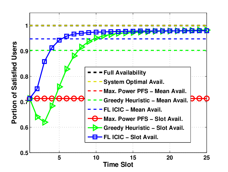
However, fuzzy logic is able to perform, on average, within 4% of the optimum throughput performance, and in fact the difference after 20 time slots (i.e., two lte frames) is less than 2%. Furthermore, it is clear that the average throughput of fuzzy logic is improved over the greedy heuristic (by 4%), even though after 15 time slots the performance is similar. This highlights that fuzzy logic icic is optimal on a cell-individual basis, however is able to (due to other inputs such as rate requirement and desired signal strength) converge to this optimum much quicker66 6 The substantial decline in performance by the greedy heuristic in the first time slots results from the lack of interference information. The unused rb with “zero” interference are allocated in all cells simultaneously, thus causing large outages in these slots. After more accurate statistics have been received, the performance improves as expected.. On the other hand, the performance difference to the optimum is minute, and therefore fuzzy logic icic provides a “near-optimal” solution for the network as a whole.
The same trends can be seen for the system availability, where while the optimum is clearly full availability (i.e., ), fuzzy logic icic achieves 98% coverage, and hence produces almost negligible outage. Furthermore, it is able to reach this availability much faster than the greedy heuristic, indicating that fuzzy logic icic employs a balance between system-wide optimisation and cell-individual performance.
IV-D Complexity
To conclude our comparison, we analyse the complexities of the three schemes, to highlight the simplicity and efficiency of our fuzzy logic technique. In a cell where fuzzy logic icic is applied, inputs (see Fig. 2) are combined at each of rb available at the fbs, inducing a complexity of . Following this, the rb are sorted according to their fuzzy score, in order to allocate the most appropriate to the ms. Since, in general, sorting algorithms demonstrate complexity, the fuzzy logic complexity within a cell increases to . Finally, given a scenario with ms, the system complexity of fuzzy logic icic is given by
The greedy heuristic utilises a similar methodology as fuzzy logic, in that it also computes a “score” (in this case the instantaneous sinr) for each rb and then orders them for allocation. Hence, the evaluation complexity at each rb is (where in this case inputs), the sorting complexity is and the overall complexity is given by
For the optimisation problem (34), finding the solution complexity is more challenging than for the heuristics, as the problem is considered -hard [26]. In general, -hard problems are only solvable (if possible) in exponential time. Here, we want to simultaneously find the resource allocation of ms, each wishing to allocate of the rb available to it. In the worst-case, an exhaustive search must be performed where all allocation possibilities at the ms must be tested. Therefore, we estimate the complexity of (34) as
This is clearly much greater than the complexity of the two heuristics, which is expected. A comparison of the achieved throughputs and required complexities77 7 Due to the massive complexity of the optimisation technique, the -axis in Fig. 7 is given in dB-flops (dBf), such that results can be compared. of the three techniques is shown in Fig. 7.

It is evident that, while (34) provides the greatest system throughput, it is substantially (i.e., exponentially) more complex than both fuzzy logic and the sinr heuristic, which only suffer slightly in terms of achieved throughput. On the other hand, it is clear that fuzzy logic icic provides enhanced throughput and coverage for the system compared to the greedy heuristic, even though the complexities are very similar. Hence, we conclude that fuzzy logic provides low-complexity, near-optimal system performance in an autonomous and distributed manner.
V Simulation
Monte Carlo simulations are used to provide performance statistics of the system with fuzzy logic icic and two benchmarks. The simulator is built following lte specifications.
V-A Scenario Construction and User Distribution
A apartment grid is considered for the simulation environment with (see Fig. 1), and is constructed as described in Section II-A. In order to obtain statistically relevant results, the random effects from ms/bs placement, lognormal shadowing and frequency selective fading must be removed. Therefore, 2000 scenarios (with minimum three fbs) are simulated and the results combined to acquire mean performance statistics of the system.
V-B Resource Allocation
Each ms is assigned two transmission requirements: a desired throughput and mcs. The desired rate of each user is drawn from a random distribution88 8 The distribution can be dependent on the scenario and traffic/applications (i.e., internet, mobile TV, etc.) desired by the users. with mean . Due to this, each msu will require a different number of rb , and hence the system will function best when strongly interfering fbs are assigned orthogonal resources.
The mcs is also assigned randomly, with equal probabilities for all available symbol efficiencies. While this is not the most realistic assumption99 9 When la is applied, the user’s mcs will more accurately reflect its sinr conditions. Furthermore, the number of rb requested will clearly change dependent on the modulation order selected., it has been applied here to further randomise the number of rb each ms needs to achieve its rate.
Finally, rb are allocated individually in each cell by the fbs. In the benchmarks, a pfs is used for rb assignment, which improves the frequency diversity relative to a random allocation. On the other hand, the fuzzy logic icic technique autonomously allocates rb based on the local information available, in order to optimise the ms(s) performance in the cell. For our purposes, the allocation of rb to ms is performed greedily, as described in Section III-C.
V-C Time Evolution
Each run of the Monte Carlo simulation is iterated over subframes, or, equivalently, lte frames, such that long-term sinr statistics can be gathered. Due to the random user and fbs distribution, plentiful runs with different network generations are considered in order to obtain statistically accurate results. At the start of each subframe, the scheduling and allocation of rb is reperformed. The ms are assumed to be quasi-static for the duration of a run.
The simulation is performed for a constant-traffic model, where each user requests the same number of rb in each time slot (i.e., subframe). Furthermore, the users are assumed to be static for the duration of a subframe, such that effects due to Doppler spread can be neglected. Perfect synchronisation in time and frequency is assumed, such that intra-cell interference is avoided. The relevant simulation parameters can be found in Table IV.
| Parameter | Value |
| Apartment width, | |
| fbs probability, | 0.5 |
| Number of available rb, | 50 |
| rb bandwidth, | |
| Average rate, | Mbps |
| Subcarriers per rb, | 12 |
| Symbol rate per subcarrier, | |
| Time slots | 25 |
| abs prob., | 0.1 |
| Spectral noise density, | |
| Total fbs transmit power | |
| Channel parameters | 97, 30 |
| Shadowing Std. Dev., | |
| Auto-correlation distance | |
V-D Benchmarks
To evaluate the performance of fuzzy logic icic, two well-known benchmark systems have been implemented for comparison purposes. These are:
- •
Maximum Power Transmission: In the first benchmark, no power allocation is performed, and all ms transmit at the maximum power on each rb.
- •
Random abs Transmission: In the second benchmark, again all links transmit at full power, however, in each time slot a user transmits an abs with probability , where for this simulation .
VI Results and Discussion
From the simulation, the statistics of the system throughput, energy efficiency, availability and fairness are generated for systems employing fuzzy logic icic and compared against the two benchmark systems. General simulation parameters are taken from Table IV and [28].
It is clear from Fig. 8 that fuzzy logic icic provides substantially improved system performance over both benchmark techniques. Especially in terms of system throughput, where the fuzzy logic schemes are the only techniques which achieve the overall desired rate (i.e., sum of individual desired rates). In fact, fuzzy logic substantially overachieves the sum desired rate, indicating almost maximum coverage and all but negligible outage. The additional rate results from the discrete allocation of bandwidth (i.e., rb), and hence the achieved user rate is generally slightly greater than what was desired. With la this becomes even more apparent, as with higher spectral efficiency the throughput “overshoot” becomes even greater.


The abs performance is constant over all time slots (except the first), as the probability of abs transmission(s) is identical in each slot. Hence, in each time slot , on average, of the users transmit an abs, providing some interference mitigation for the remaining users. This abstinence of data transmission explains the throughput losses by the abs system relative to full power transmission, as clearly the interference mitigation provided is less significant than the throughput sacrificed.
Fig. 8 also displays the energy efficiency of the simulated scenario, yielding again very dominant results of the fuzzy logic systems. This is mainly due to the fact that fuzzy logic has the possibility of transmitting at half power, which is usually the case after multiple time slots and the achievement of a relatively orthogonal rb allocation. Furthermore, the high energy efficiency is achieved quite rapidly. The added energy efficiency due to la is a direct result of the augmented throughputs (see (6)). It is shown that abs transmission is slightly more energy efficient than maximum power transmission, which is logical since on average 10 less power is used, but the loss in throughput is , thus enhancing the energy efficiency.


Lastly, the availability and throughput fairness in the system are investigated. As expected, fuzzy logic icic/la provides by far the best ms availability, as can be seen from Fig. 9, achieving availability. This is expected as both the system throughputs are augmented, a direct result of the greater portion of satisfied ms. Furthermore, it is clear that the fairness is greatly improved as well, especially when utilising la. This is mainly due to the fact that users are (through la) more adept to their transmission environments, and hence better achieve their desired rates1010 10 In fact, due to the reduced throughput granularity at higher mcs, more ms achieve the same throughput, and hence fuzzy logic icic/la achieves a greater fairness than if all ms would exactly achieve their targets.. On another note, the max. power availability and fairness is boosted with regards to the abs system, as all ms can transmit without restrictions or abstinence, and hence even unsatisfied (in terms of rate) users achieve decent throughputs. A summary of the quantitative results is shown in Table V.
| %-gain | vs. | Throughput | Energy Eff. | Availability | Fairness |
|---|---|---|---|---|---|
| FL. ICIC/LA | Max. Power | 57 | 151 | 59 | 33 |
| FL. ICIC | Max. Power | 38 | 103 | 48 | 29 |
| FL. ICIC/LA | ABS | 68 | 143 | 70 | 44 |
| FL. ICIC | ABS | 48 | 97 | 59 | 40 |
| FL. ICIC/LA | FL. ICIC | 14 | 24 | 7 | 3 |
VII Conclusions
In this paper, a distributed and autonomous icic technique for femto-femto interference management and resource allocation is presented. At each fbs, locally available information is utilised to evaluate the allocatability of the available rb in a particular cell, taking into account the interference neighbourhood, user rates, and the own-cell signal and fading environment. Fuzzy logic generates broad evaluations of these inputs, combines them based on a defined set of rb allocation rules, and submits to the bs the most suitable resources and transmit powers for successful and efficient communication. After several time slots and more accurate average signal statistics, the locally optimised resource allocations form a near-optimal global solution.
By comparing fuzzy logic icic to a system-wide optimisation problem, it was shown that fuzzy logic provides close-to-optimal system performance with drastically reduced complexity. Furthermore, a comparison to a greedy heuristic of similar complexity shows faster convergence to cell-individual optimum resource allocation. Hence, fuzzy logic provides a low-complexity near-system-optimal solution of icic in femto-cell networks. This is confirmed in the simulation results, where fuzzy logic icic satisfies the system throughput requirements and significantly outperforms the given benchmarks. The addition of la gives a further performance boost, achieving almost full availability along with enhanced throughput, energy efficiency, and fairness.
The main focus of the further development of fuzzy logic icic is the extension to hetnet, as highlighted in Section I. This will see macro-, pico- and femto-cells available in the same scenario, thus the ms will not only need to perform resource and power allocation, but also determine which ap they desire to connect with. The autonomous and distributed nature of fuzzy logic icic should allow these networks to self-configure, and self-optimise, eliminating excessive signalling normally required in such networks. Furthermore, we seek to heuristically optimise the fuzzy logic system (i.e., more specifically, the rules) by analysing the input-output characteristics, and tuning the system to make better decisions on each rb.
References
- [1] D. Lopez-Perez, I. Guvenc, G. de la Roche, M. Kountouris, T. Quek, and J. Zhang, “Enhanced intercell interference coordination challenges in heterogeneous networks,” IEEE Wireless Communications, vol. 18, no. 3, pp. 22 –30, Jun. 2011.
- [2] G. Boudreau, J. Panicker, N. Guo, R. Chang, N. Wang, and S. Vrzic, “Interference Coordination and Cancellation for 4G Networks,” IEEE Communications Magazine, vol. 47, no. 4, pp. 74–81, 2009.
- [3] D. Astely, E. Dahlman, A. Furuskar, Y. Jading, M. Lindstrom, and S. Parkvall, “LTE: The Evolution of Mobile Broadband,” IEEE Communications Magazine, vol. 47, no. 4, pp. 44–51, 2009.
- [4] R. Madan, J. Borran, A. Sampath, N. Bhushan, A. Khandekar, and T. Ji, “Cell association and interference coordination in heterogeneous lte-a cellular networks,” IEEE Journal on Selected Areas in Communications, vol. 28, no. 9, pp. 1479 –1489, Dec. 2010.
- [5] S.-M. Cheng, S.-Y. Lien, F.-S. Chu, and K.-C. Chen, “On exploiting cognitive radio to mitigate interference in macro/femto heterogeneous networks,” IEEE Wireless Communications, vol. 18, no. 3, pp. 40 –47, Jun. 2011.
- [6] P. Hasselbach, A. Klein, and I. Gaspard, “Transmit Power Allocation for Self-Organising Future Cellular Mobile Radio Networks,” in Proc. of IEEE 20th International Symposium on Personal, Indoor and Mobile Radio Communications (PIMRC), Sep. 2009, pp. 1342 –1346.
- [7] D. Gesbert, S. G. Kiani, A. Gjendemsjø, and G. E. Øien, “Adaptation, Coordination, and Distributed Resource Allocation in Interference-Limited Wireless Networks,” Proc. of the 7th IEEE International Symposium on Wireless Communication Systems, vol. 95, no. 12, pp. 2393–2409, Dec. 2007.
- [8] Y.-Y. Li, M. Macuha, E. Sousa, T. Sato, and M. Nanri, “Cognitive interference management in 3g femtocells,” in Proc. of IEEE 20th International Symposium on Personal, Indoor and Mobile Radio Communications (PIMRC), Sep. 2009, pp. 1118 –1122.
- [9] L. Lindbom, R. Love, S. Krishnamurthy, C. Yao, N. Miki, and V. Chandrasekhar, “Enhanced Inter-cell Interference Coordination for Heterogeneous Network in LTE-Advanced: A Survey,” Tech. Rep., 2011.
- [10] J. Pang, J. Wang, D. Wang, G. Shen, Q. Jiang, and J. Liu, “Optimized time-domain resource partitioning for enhanced inter-cell interference coordination in heterogeneous networks,” in Proc. of Wireless Communications and Networking Conference (WCNC), Apr. 2012, pp. 1613 –1617.
- [11] A. Stolyar and H. Viswanathan, “Self-Organizing Dynamic Fractional Frequency Reuse for Best-Effort Traffic through Distributed Inter-Cell Coordination,” in Proc. of IEEE INFOCOM, Apr. 2009, pp. 1287–1295.
- [12] R. Combes, Z. Altman, M. Haddad, and E. Altman, “Self-Optimizing Strategies for Interference Coordination in OFDMA Networks,” in Proc. of IEEE International Conference on Communications (ICC) Workshops, no. 1–5, Jun. 2011.
- [13] L. Jouffe, “Fuzzy inference system learning by reinforcement methods,” IEEE Transactions on Systems, Man, and Cybernetics, Part C: Applications and Reviews, vol. 28, pp. 338–355, Aug. 1998.
- [14] M. Dirani and Z. Altman, “A cooperative Reinforcement Learning approach for Inter-Cell Interference Coordination in OFDMA cellular networks,” in Proc. of Modeling and Optimization in Mobile, Ad Hoc and Wireless Networks (WiOpt), May 2010, pp. 170–176.
- [15] P. Vlacheas, E. Thomatos, K. Tsagkaris, and P. Demestichas, “Autonomic downlink inter-cell interference coordination in LTE Self-Organizing Networks,” in Proc. of Network and Service Management (CNSM), Oct. 2011, pp. 1–5.
- [16] R. Razavi, S. Klein, and H. Claussen, “Self-optimization of capacity and coverage in LTE networks using a fuzzy reinforcement learning approach,” in Proc. of Personal Indoor and Mobile Radio Communications (PIMRC), Sep. 2010, pp. 1865–1870.
- [17] S. Sesia, I. Toufik, and M. Baker, LTE - The UMTS Long Term Evolution: From Theory to Practice, 1st ed., S. Sesia, I. Toufik, and M. Baker, Eds. Wiley, 2009.
- [18] EDX Wireless, “Designing an LTE network using EDX SignalPro,” Technical white paper, march 2010, retrieved Jan. 17 2011. [Online]. Available: http://www.edx.com/resources/documents/
- [19] R. Jain, D. Chiu, and W. Hawe., “A Quantitative Measure of Fairness and Discrimination for Resource Allocation in Shared Computer Systems,” DEC Technical Report, Tech. Rep. 301, 1984.
- [20] Z. Bharucha, H. Haas, A. Saul, and G. Auer, “Throughput Enhancement through Femto-Cell Deployment,” European Transactions on Telecommunications, vol. 21, no. 4, pp. 469–477, Mar. 31 2010, (invited). [Online]. Available: http://www.interscience.wiley.com
- [21] ITU-R Working Party 5D (WP5D) - IMT Systems, “Report 124, Report of correspondence group for IMT.EVAL,” May 2008, United Arab Emirates.
- [22] W. Wang, T. Ottosson, M. Sternad, A. Ahlen, and A. Svensson, “Impact of Multiuser Diversity and Channel Variability on Adaptive OFDM,” in Proc. of the 58th IEEE Vehicular Technology Conference (VTC-Fall), Orlando, USA, Oct. 6-9 2003, pp. 547–551.
- [23] NTT DOCOMO, “New Evaluation Models (Micro Cell, Indoor, Rural/High-Speed),” 3GPP TSG RAN WG1 R1-082713, Jul. 2008. Retrieved Nov. 27, 2009 from www.3gpp.org/ftp/tsg_ran/WG1_RL1/TSGR1_53b/Docs/.
- [24] 3GPP, “Simulation Assumptions and Parameters for FDD HeNB RF Requirements,” 3GPP TSG RAN WG4 R4-092042, May 2008. Retrieved Sep. 1, 2009 from www.3gpp.org/ftp/Specs/.
- [25] S. Almalfouh and G. Stüber, “Interference-Aware Radio Resource Allocation in OFDMA-Based Cognitive Radio Networks,” IEEE Transactions on Vehicular Technology, vol. 60, no. 4, pp. 1699 –1713, May 2011.
- [26] D. P. Bertsekas, Nonlinear Programming. Athena Scientific, 1999.
- [27] M. Trott, “The Mathematica Guidebooks Additional Material: Average Distance Distribution,” Oct. 2004.
- [28] 3GPP, “X2 General Aspects and Principles (Release 8),” 3GPP TS 36.420 V8.0.0 (2007-12), Dec. 2007. Retrieved Sep. 1, 2009 from www.3gpp.org/ftp/Specs/.