High–Order Asymptotic–Preserving Methods
for
fully nonlinear relaxation problems

Relaxation effects are an important feature of models arising, for instance, in compressible fluid dynamics and, specifically, we are interested here in nonlinear hyperbolic systems with fully nonlinear relaxation terms in the limit of, both, infinitely stiff relaxation and arbitrarily late time. In this limit, the dynamics of the flow is governed by effective systems of parabolic type, whose diffusion might also be degenerate and/or fully nonlinear. Solving such equations numerically is very challenging due to the stiffness of the problem in, both, the convection and the relaxation parts. This problem is currently under very active study and the main challenge is to design schemes that allow for realistic stability conditions on the time–step while ensuring robustness and high–order accuracy. For background as well as recent material, we refer to [2, 8, 14, 13, 18, 20].

The simplest example of interest, which we propose to refer to as the linear relaxation model, reads

in which $u=u(t,x)$ and $v=v(t,x)$ are the unknown functions, and $b=b(u)$ and $q=q(u)$ are prescribed with $b^{\prime}(u)>0$. This is a nonlinear hyperbolic system with two (distinct and real) characteristic speeds, that is, $\pm\sqrt{b^{\prime}(u)}/\epsilon$. In the stiff relaxation limit $\epsilon\to 0$, the characteristic speeds approach infinity and the behavior of solutions to (1) is (formally, at least) governed by the effective system

which can be derived by a Chapman–Enskog expansion in the parameter $\epsilon$ and turns out to be a noninear parabolic system —since the diffusion coefficient $b^{\prime}(u)>0$ in $(b^{\prime}u)u_{x})_{x}$ is positive. Observe that the so-called sub–characteristic condition [23] for system (2) reads $\epsilon\,|q^{\prime}(u)|<(b^{\prime}(u))^{1/2}$ and puts a restriction on the speed $q^{\prime}(u)$ of the effective equation with respect to the speeds $\pm\sqrt{b^{\prime}(u)}/\epsilon$ of the original system: clearly, for this model, the sub–characteristic condition is automatically satisfied (for $\epsilon$ sufficiently small).

Fully nonlinear relaxation terms also arise (for instance in presence of nonlinear friction) and, therefore, in this work we also numerically study the following nonlinear relaxation model, first introduced by Kawashima and LeFloch [15],

where $m>0$ is a real parameter. This, again, is a strictly hyperbolic system of balance laws, provided $b^{\prime}(u)>0$. The effective system associated with this model is found to be (with $\alpha=-1+1/m$)

which is a fully nonlinear parabolic equation in $u$. It is natural to distinguish between three rather distinct behaviors:

The equation (4), although parabolic in nature, need not regularize initially discontinuous initial data, and we may expect jump singularities (in the first–order derivative $u_{x}$) to remain in the late–time limit.

Further models arising in compressible fluid dynamics will also be described later, but (1) and (3) provide us two prototypes of particular importance in order to develop efficient numerical tools for relaxation problems.

IMEX R–K schemes present in the literature can be classified in three different types characterized by the structure of the matrix $A=(a_{ij})_{i,j=1}^{s}$ of the implicit scheme. Following [3], we will rely on the following notions.

The schemes CK are very attractive since they allow some simplifying assumptions, that make order conditions easier to treat, therefore permitting the construction of higher order IMEX R–K schemes. On the other hand, schemes of type A are more amenable to a theoretical analysis, since the matrix A of the implicit scheme is invertible.

The simplest IMEX-RK are obtained combining explicit and implicit Euler method. Two versions are possible applied to system (6), namely

The corresponding Butcher tables are reported below:

In general, Implicit–Explicit (IMEX) Runge–Kutta (R–K) schemes [1, 3, 4, 9, 21] represent a powerful tool for the time discretization of stiff systems. However, in the hyperbolic–to–parabolic limit under consideration here, the characteristic speeds of the hyperbolic part is of order $1/\epsilon$ and standard IMEX Runge–Kutta schemes developed for hyperbolic problems with stiff relaxation [21, 7] are not very efficient, since the standard CFL condition requires the relation $\Delta t=\mathcal{O}(\epsilon\Delta x)$ between the time mesh–size and the space mesh–size. Clearly, in the diffusive regime $\epsilon<<\Delta x$, and we are led to a too restrictive condition, since it is expected that, for an explicit method, a parabolic–type stability condition $\Delta t=\mathcal{O}(\Delta x^{2})$ should suffice.

Most existing works [13, 14, 20] on asymptotic preserving schemes for nonlinear hyperbolic system with diffusive relaxation are based on a (micro–macro) decomposition of the hyperbolic flux into stiff and non–stiff components: the stiff hyperbolic component is added to the relaxation term, which is treated implicitly; in the limit of infinite stiffness, such schemes become consistent and explicit schemes for the diffusive limit equation [14, 16, 17, 19, 20] and, therefore, suffer from the usual stability restriction $\Delta t=\mathcal{O}(\Delta x^{2})$.

Schemes that do avoid the parabolic time–step restriction and provide fully implicit solvers (in the case of transport equations) have been analyzed in [6], where a new formulation of the problem (1) in the case $b(u)=u$ and $q(u)=0$, was introduced, which was based on the addition of two opposite diffusive terms in the stiff limit. One term is added to the hyperbolic component and makes it non–stiff (therefore allowing for an explicit treatment), while the other term must be treated implicitly. The remaining component of the hyperbolic term is formally treated implicitly. The resulting scheme is consistent and relaxes to an implicit scheme for underlying diffusion limit, therefore avoiding the typical parabolic restriction of previous methods.

The drawback of the above strategy is that its requires an implicit treatment of some components of the hyperbolic flux. Even if such implicit term can be computed by closed formula in most cases, this procedure requires a reformulation of the discretization of the whole system. It is thus desirable to construct IMEX R–K schemes in which the whole hyperbolic part is treated explicitly. At a first sight this seems an impossible task since the characteristic speeds are unbounded. Yet, in [8], the authors showed that, provided suitable conditions are imposed on the IMEX R–K coefficients, then one can indeed construct schemes which are

• •

  fully explicit in the hyperbolic part, and

• •

  converge to an implicit high–order scheme in the diffusion limit.

This is this direction that we follow in the present work and further develop in the context of, both, the linear relaxation model (1), the fully nonlinear model (3), and several models arising in fluid dynamics. We exhibit new decompositions that lead us to high–order asymptotic preserving methods covering the hyperbolic–to–parabolic regime under consideration. A key ingredient is to keep the implicit feature of the scheme with respect to certain components that “degenerate”; for instance, (3) when $m>1$ has a degenerate diffusion when $-q(u)+b(u)_{x}$ is small or even vanishes.

The schemes constructed with the approachs outlined above will converge to an explicit scheme for the limit diffusion equation, and therefore they are subject to the classical parabolic CFL restriction $\Delta t\leq C\Delta x^{2}$. In order to overcome such a restriction we adopt a penalization technique, based on adding two opposite terms to the first equation, and treating one explicitly and one implicitly.

Let us consider system (1) and adding and subtracting the same term $\mu(\varepsilon)b(u)_{xx}$ on the right hand side we obtain:

Here $\mu=\mu(\varepsilon)\in[0,1]$ is a free parameter such that $\mu(0)=1$. The idea is that, since the quantity $v+b(u)_{x}$ is close to $q(u)$ as $\varepsilon\to 0$, the first term on the right hand side can be treated explicitly in the first equation, while the term $p(u)_{x}x$ will be treated implicitly. This can be done naturally by using an IMEX R–K approach.

However, if we want the scheme to be accurate also in the cases in which $\varepsilon$ is not too small, then we need to add two main ingredients:

• 1.

  no term should be added when not needed, i.e. for large enough values of $\varepsilon$, since in such cases the additional terms degrade the accuracy; this can be achieved by letting $\mu(\varepsilon)$ decrease as $\varepsilon$ increases. A possible choice, for example, is

  $$\mu(\varepsilon)=\exp(-\varepsilon^{2}/\Delta x).$$

• 2.

  when the stabilizing effect of the dissipation vanishes, i.e. as $\mu\to 0$, then central differencing is no longer suitable, and one should adopt some upwinding; this can be obtained for example by blending central differencing and upwind differencing as

  $$D_{x}=(1-\mu)D_{x}^{\rm upw}+\mu D_{x}^{\rm cen}.$$

Now from a numerical point of view, we may treat system (17) in two different approaches according to whether the hyperbolic term $b(u)_{x}$ in the second equation is treated implicitly or explicitly. The first one, called the BPR approach (For more details as well as some rigorous analysis, see [6].) is

and the corresponding IMEX R–K schemes are IMEX-I R–K ones in order to remind that the term containing $b(u)_{x}$ in the second equation is implicit, in the sense that it appears at the new time level. Observe that the term $b(u)_{x}+v-q(u)$ appearing in the second equation is formally treated implicitly, but in practice the term $b(u)_{x}$ is computed at the new time from the first equation, so it can in fact explicitly computed.

The second approach (cf. [8] for further details) is given by

which is refered to as the BR approach; he corresponding schemes are IMEX-E.

Observe that when $q(u)\neq 0$, the system relaxes to a convection–diffusion equation. The terms on the left hand side are treated explicitly, while the terms on the right–hand side are treated implicitly. In fact as $\epsilon\to 0$, the scheme becomes an IMEX R–K scheme for the limit convection-diffusion equation, in which the convection term is treated explicitly and the diffusion one is treated implicitly [6, 8].

In [6, 8] additional order conditions, called algebraic conditions are derived by studying the behavior of IMEX R–K schemes applied to the relaxation system (17) when $\epsilon\to 0$, in particular when $\epsilon=0$. These algebraic conditions guarantee the correct behavior of the numerical solution in the limit $\varepsilon\to 0$ and maintain the accuracy in time of the scheme. We obtained such algebraic order conditions using the same technique adopted in [4], i.e.  by comparing the Taylor series of the numerical solution with that of the exact solution.

In [6] these order conditions are derived for IMEX-I R–K schemes and in [8] for IMEX-E R–K ones. Due to the number of these order conditions, it is necessary to use several internal levels for IMEX R–K schemes in order to obtain a given order. Several results and a rigorous analysis about that can be found in [6, 8]. Most numerical tests are reported in [6] for the BPR approach and in [8] for the BR approach and the results are compared with those obtained by other methods available in the literature.

Here we report, as an example, the application of the second order IMEX-E R–K scheme developed in [8] and called AGSA(3,4,2). We note that this scheme satisfy all the algebraic order conditions derived in [8]. Now we perform several numerical tests, considered earlier in [2] with a different numerical strategy.

We are now in a position to tackle the nonlinear relaxation model (3) which is of central interest in the present paper. Without genuine loss of generality in the design of the numerical method, we assume that $b(u)=u$ and $q(u)=0$ and, therefore, we study

together with the associated effective equation ($\varepsilon\to 0$)

with $\alpha=-1+1/m$.

The order of convergence of the IMEX scheme applied to the semilinear system (49) for small $\varepsilon$ will be determined by comparing the numerical solutions to a (theoretical) limiting solution obtained by solving the effective equations (50) on a very fine mesh.

We are going to treat the nonlinear relaxation term implicitly, which requires to solve a nonlinear algebraic equation. An efficient approach is obtained by solving it iteratively with the Newton method. Specifically, the nonlinear equation to be solved at each $s$–stage has the form

where $C_{1}$ and $C_{2}$ constants. As $\varepsilon\to 0$, we can neglect the term $V\varepsilon^{2}$ and, therefore, we propose the initial approximation

as a good choice in order to reduce the number of iterations. This is a relevant choice in both cases $m<1$ and $m\geq 1$.

Equation (50) is a nonlinear diffusion equation. Let us introduce a very efficient method for the numerical solution of such an equation. The scheme we propose is stable, linearly implicit, and can be designed up to any order of accuracy. We propose to use a technique similar to the additive semi-implicit Runge-Kutta methods of Zhong [24]. The idea is to write equation as a system

where the first argument is treated explicitly, while the second one is treated implicitly. Then the semi-implicit R–K method is implemented as follows. First compute the stage fluxes for $i=1,\ldots,s$

solve the equation

and, finally update the numerical solution

In our case $F(u^{\ast},u)$ is given by

It can be shown that such semi-implicit R–K scheme is indeed a particular case of IMEX R–K scheme [22].

Observe that, for the spatial discretization of the limiting equation (50), we can use a centered scheme, such as

where $|\delta U|^{\alpha}_{j+\frac{1}{2}}=\Big|\frac{U_{j+1}(t)-U_{j}(t)}{\Delta x}\Big|^{\alpha}$. Observe that for the final numerical solution, we require, in particular, that $u^{\ast^{n+1}}=u^{n+1}$, which is guaranteed by imposing the condition $b_{i}=\widetilde{b}_{i}$ for all $i$.

Here, as an example, we propose to choose a classical second–order IMEX R–K scheme that satisfies the condition $b_{i}=\widetilde{b}_{i}$ for all $i$, e.g. the implicit–explicit midpoint method of type ARS introduced in [1] (to which we refer for further details). Applying such a method, we thus obtain the following (rather simple) scheme which requires only two function evaluations

Observe that $\mathcal{U}^{\ast}_{1}=\mathcal{U}_{1}=u_{n}$.

Similar examples is possible to propose for other types of IMEX R–K schemes presented in the literature. Then, we consider the numerical solution (54) as a reference solution for the limiting equation, and we compare it with the numerical one computed from the system (49).

Here we apply first order scheme to system (49) with simple second order central differencing for the discretization of the space derivative. We choose the first order implicit-explicit Euler scheme of type ARS (2.2). For our numerical test we integrate the system up to the final time $T=1$ and use periodic boundary conditions in $x\in[-\pi,\pi]$ with initial conditions $u(x,0)=\cos x$, $v(x,0)=\sin x$ and $\varepsilon=10^{-4}$.

Numerical convergence rate is calculated by the formula

where $E_{\Delta t_{1}}$ and $E_{\Delta t_{2}}$ are the global errors computed with step $\Delta t_{1}=\mathcal{O}(\Delta x_{1}^{2})$ where $\Delta x_{1}=2\pi/N$ and $\Delta t_{2}=\mathcal{O}(\Delta x_{2}^{2})$ with $\Delta x_{2}=\pi/N$.

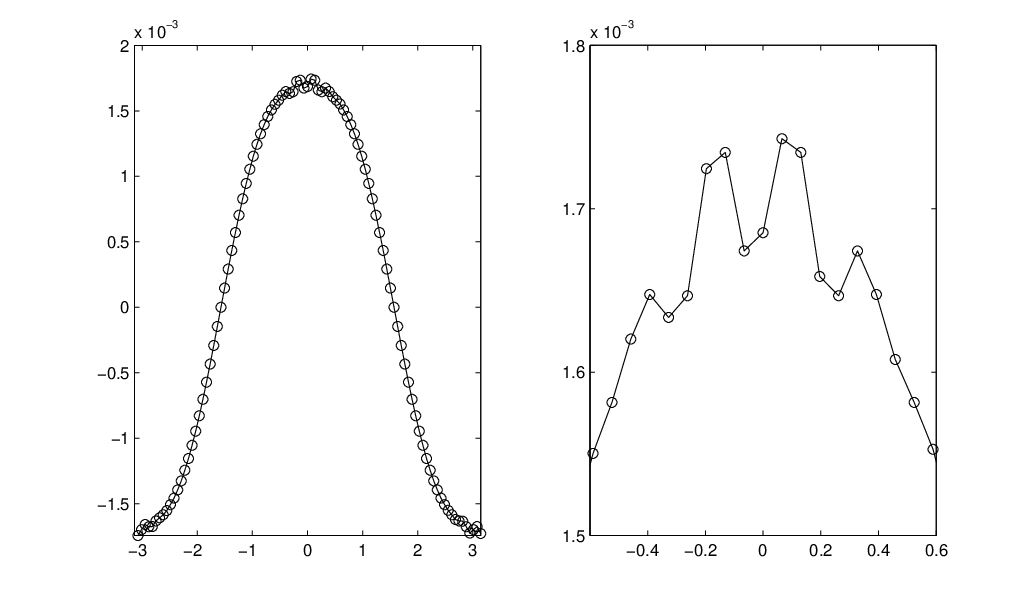
The nonlinear parabolic equation (50) has regular solutions if $m\geqslant 1$, i.e. $\alpha\leqslant 0$, while it develops singularities in the derivatives if $0<m<1$, i.e. $\alpha>0$. Two value of $m$ are considered here, namely $m=1/2$ ($\alpha=1$) and $m=2$ ($\alpha=-1$). The profile of the solution computed with $N=96$ points is reported in Fig. 3. The time step has been chosen to satisfy $\Delta t=C\Delta x^{2}$, with $C=0.025$ (right panel with $m=2$) and $C=1$ (left panel with $m=1/2$). The scheme seems to converge in both cases.

Using $N=12\cdot 2^{p}$ with $p=0,1,...,5$, one obtains the convergence table 1. The $L^{\infty}$ convergence is second order for $m=2$, and less for $m=0.5$, as expected from the lack of regularity of the solution. Convergence rate in the latter case improves when measured in slightly weaker norms, i.e. $L^{1}$ and $L^{2}$ norm. Observe that second–order is observed even if the scheme is first–order in time, which is due to the parabolic scaling of the time step.

Let us take a closer look at the case $m=2$. By integrating for a longer time, some instabilities appear (see Fig. 4). The reason of such instabilities is that the following equation (50) may be written in the form

where the low order term $(\alpha+1)|u_{x}|^{\alpha}$ plays the role of the diffusive coefficient.

It can be shown [8] that the first order Implicit-Explicit Euler scheme applied to the linear system (49) suffers from the following stability restriction, independently of $\varepsilon$

which suggests the following condition in the nonlinear case

This condition is used to determine the optimal time step for $m\leqslant 1$, while it shows that no time step can guarantee stability near local extrema if $m>1$. For this reason, it is strictly necessary to use implicit schemes when $m>1$.

As we have seen, the previous numerical example outlined above converges to an explicit scheme for the limit diffusion equation, and therefore subjected to the classical parabolic CFL restriction $\Delta t\leqslant C\Delta x^{2}$. Furthermore in some cases such restriction does not allow the computation of the solution, due to the unboundedness of the diffusion coefficient.

Now, in order to remove the parabolic CFL restriction we adopt a similar technique proposed for the linear relaxation model that consists in adding and subtracting the same term to the first equation. In the nonlinear model equation (3), with $q(u)=0$, $b(u)=u$, the system becomes

Here, $\mu(\epsilon)$ is such that $\mu:\mathbb{R}^{+}\to[0,\ 1]$ and $\mu(0)=1$. When $\epsilon$ is not small there is no reason to add and subtract the term $\mu(\epsilon)u_{xx}$, therefore $\mu(\epsilon)$ will be small in such a regime, i.e. $\mu(\epsilon)=0$.

We note that in both the BR and BPR approach the term $(|u_{x}|^{\alpha}u_{x})_{x}$ is treated implicitly. In the case of a fully implicit treatment of such term, both approaches can be used. Of course the BR approach requires that the Runge-Kutta IMEX is globally stiffly accurate [6, 8].

If, on the other hand, we want to use the treatment of the implicit term by the technique outlined in section 6.2, then we are forced to use BPR approach, since the requirement that $b=\tilde{b}$ cannot reconcile with global stiff accuracy. To be more specific, in our case $F(y^{\ast},y)$ is given by $y=\left(\begin{array}[]{l}u\\ v\end{array}\right),\,y^{\ast}=\left(\begin{array}[]{l}u^{\ast}\\ v^{\ast}\end{array}\right),$ and

It can be shown that such semi-implicit R–K scheme is indeed a particular case of IMEX R–K scheme (Pareschi, Russo, private communication). Furthermore, if $\tilde{c}=\tilde{A}e=c=Ae$, the classical order conditions on the two schemes

References

- [1] U. Ascher, S. Ruuth, and R.J. Spiteri, Implicit-explicit Runge–Kutta methods for time dependent partial differential equations, Appl. Numer. Math. 25 (1997), 151–167.
- [2] C. Berthon, P.G. LeFloch, and R. Turpault, Late–time relaxation limits of nonlinear hyperbolic systems. A general framework, Math. of Comput. (2012). See also ArXiv:1011.3366.
- [3] S. Boscarino, Error analysis of IMEX Runge–Kutta methods derived from differential algebraic systems, SIAM J. Numer. Anal. 45 (2007), 1600–1621.
- [4] S. Boscarino, On an accurate third order implicit–explicit Runge-Kutta method for stiff problems, Appl. Num. Math. 59 (2009), 1515–1528.
- [5] S. Boscarino, F. Filbet, and G. Russo, in preparation.
- [6] S. Boscarino, L. Pareschi, and G. Russo, Implicit–explicit Runge–Kutta schemes for hyperbolic systems and kinetic equations in the diffusion limit, SIAM J. Sc. Comp., accepted for publication.
- [7] S. Boscarino and G. Russo, On a class of uniformly accurate IMEX Runge–Kutta schemes and application to hyperbolic systems with relaxation, SIAM J. Sci. Comput. 31 (2009), 1926–1945.
- [8] S. Boscarino and G. Russo, Flux–explicit IMEX Runge–Kutta schemes for hyperbolic to parabolic relaxation problems, SIAM J. Num. Anal., accepted for publication.
- [9] M.H. Carpenter and C.A. Kennedy, Additive Runge–Kutta schemes for convection–diffusion–reaction equations, Appl. Numer. Math. 44 (2003), 139–181.
- [10] F. Cavalli, G. Naldi, G. Puppo, and M. Semplice, High order relaxation schemes for nonlinear diffusion problems, SIAM J. Numer. Anal. 45 (2007), 2098–2119.
- [11] E. Hairer, S.P. Norsett, and G. Wanner, Solving Ordinary Differential Equation. I. Non-stiff problems, Springer Series in Comput. Mathematics, Vol. 8, Springer Verlag, (2nd edition), 1993.
- [12] E. Hairer and G. Wanner, Solving Ordinary Differential Equation. II. Stiff and differential algebraic problems, Springer Series in Comput. Mathematics, Vol. 14, Springer Verlag, (2nd edition), 1996.
- [13] S. Jin and L. Pareschi, Discretization of the multiscale semiconductor Boltzmann equation by diffusive relaxation schemes, J. Comp. Phys. 161 (2000), 312–330.
- [14] S. Jin, L. Pareschi, and G. Toscani, Diffusive relaxation schemes for multiscale discrete–velocity kinetic equations, SIAM J on Numer. Anal. 35 (1998), 2405–2439.
- [15] S. Kawashima and P.G. LeFloch, in preparation.
- [16] A. Klar, An asymptotic-induced scheme for non stationary transport equations in the diffusive limit. SIAM J. Numer. Anal. 35 (1998), 1073–1094.
- [17] P. Lafitte and G. Samaey, Asymptotic–preserving projective integration schemes for kinetic equations in the diffusion limit, Preprint 2010.
- [18] P.G. LeFloch, A framework for late-time/stiff relaxation asymptotics, Proc. ” CFL condition - 80 years gone by”, Rio de Janeiro Aug. 2010, C.S. Kubrusly et al. (editors), Springer Proc. Math., 2012. See also Arxiv:1105.1415.
- [19] M. Lemou and L. Mieussens, A new asymptotic preserving scheme based on micro–macro formulation for linear kinetic equations in the diffusion limit, SIAM J. Sci. Comp. 31 (2010), 334–368.
- [20] G. Naldi and L. Pareschi, Numerical schemes for hyperbolic systems of conservation laws with stiff diffusive relaxation, SIAM J. on Numer. Anal. 37 (2000), 1246–1270.
- [21] L. Pareschi and G. Russo, Implicit–explicit Runge–Kutta schemes and applications to hyperbolic systems with relaxations, J. Sci. Comput. 1 (2005), 129–155.
- [22] L. Pareschi and G. Russo, private communication.
- [23] G. Whitham, Linear and Nonlinear Waves, Vol. 226. Wiley, New York, 1974.
- [24] X. Zong, Additive Semi-Implicit Runge-Kutta methods for computing high-speed non equilibrium reactive flows, J. Comput. Phys. 128 (1996), 19–31.