Oriented Euler Complexes and Signed Perfect Matchings
Abstract
This paper presents “oriented pivoting systems” as an abstract framework for complementary pivoting. It gives a unified simple proof that the endpoints of complementary pivoting paths have opposite sign. A special case are the Nash equilibria of a bimatrix game at the ends of Lemke–Howson paths, which have opposite index. For Euler complexes or “oiks”, an orientation is defined which extends the known concept of oriented abstract simplicial manifolds. Ordered “room partitions” for a family of oriented oiks come in pairs of opposite sign. For an oriented oik of even dimension, this sign property holds also for unordered room partitions. In the case of a two-dimensional oik, these are perfect matchings of an Euler graph, with the sign as defined for Pfaffian orientations of graphs. A near-linear time algorithm is given for the following problem: given a graph with an Eulerian orientation with a perfect matching, find another perfect matching of opposite sign. In contrast, the complementary pivoting algorithm for this problem may be exponential.
Keywords: Complementary pivoting, Euler complex, linear complementarity problem, Nash equilibrium, perfect matching, Pfaffian orientation, PPAD.
AMS 2010 subject classification: 90C33
Apart from Appendix A and Appendix B, this article is published in Mathematical Programming, Series B, DOI 10.1007/s10107-014-0770-4, accessible online at http://link.springer.com/article/10.1007/s10107-014-0770-4.
1 Introduction
A fundamental problem in game theory is that of finding a Nash equilibrium of a bimatrix game, that is, a two-player game in strategic form. This is achieved by the classical pivoting algorithm by Lemke and Howson (1964). Shapley (1974) introduced the concept of an index of a Nash equilibrium, and showed that the endpoints of every path computed by the Lemke–Howson algorithm have opposite index. As a consequence, any nondegenerate game has an equal number of equilibria of positive and negative index, if one includes an “artificial equilibrium” (of, by convention, negative index) that is not a Nash equilibrium. The Lemke–Howson algorithm is one motivating example for the complexity class PPAD defined by Papadimitriou (1994). PPAD stands for “polynomial parity argument with direction” and describes a class of computational problems whose solutions are the endpoints of implicitly defined, and possibly exponentially long, directed paths. A salient result by Chen and Deng (2006) is that finding one Nash equilibrium of a bimatrix game is PPAD-complete.
Lemke (1965) generalized the Lemke–Howson algorithm to more general linear complementary problems (LCPs). Lemke’s algorithm is the fundamental complementary pivoting algorithm; a substantial body of subsequent work is concerned with its applicability to LCPs and related problems (for a comprehensive account see Cottle, Pang, and Stone, 1992). Todd (1972; 1974) introduced a theory of “abstract” complementary pivoting where the sets of basic and nonbasic variables in a linear system are replaced by elements of a “primoid” and “duoid”.
Todd’s “semi-duoids” have been studied independently by Edmonds (2009) under the name of Euler complexes or “oiks”. A -dimensional Euler complex over a finite set of nodes is a multiset of -element sets called rooms so that any set of nodes is contained in an even number of rooms. For a family of oiks over the same node set , Edmonds (2009) showed that there is an even number of room partitions of , using an “exchange algorithm” which is a type of parity argument. A special case is a family of two oiks of possibly different dimension corresponding to the two players in a bimatrix game. Then room partitions are equilibria, and the Lemke–Howson algorithm is a special case of the exchange algorithm. In another special case, all oiks in the family are the same -oik, which is an Euler graph with edges as rooms and perfect matchings as room partitions.
This paper presents three main contributions in this context. First, we define an abstract framework called pivoting systems that describes “complementary pivoting with direction” in a canonical manner. Similar abstract pivoting systems have been proposed by Todd (1976) and Lemke and Grotzinger (1976); we compare these with our approach in Section 5. Second, using this framework, we extend the concept of orientation to oiks and show that room partitions at the two ends of a pivoting path have opposite sign, provided the underlying oik is oriented. For two-dimensional oiks, which are Euler graphs, room partitions are perfect matchings. Their orientation is the sign of a perfect matching as defined for Pfaffian orientations of graphs. Our third result is a polynomial-time algorithm for the following problem: Given a graph with an Eulerian orientation and a perfect matching, find another perfect matching of opposite sign. The complementary pivoting algorithm that achieves this may take exponential time.
In order to motivate our general framework, we sketch here two canonical examples (with further details in Section 2) where paths of complementary pivoting have a direction and endpoints of opposite sign. The first example is a simple polytope in dimension with facets, each of which has a label in . A vertex is called completely labeled if the facets it lies on together have all labels . The sign of a completely labeled vertex is the sign of the determinant of the matrix of the normal vectors of the facets it lies on when written down in the order of their labels. The “parity theorem” states that the polytope has an equal number of completely labeled vertices of positive and of negative sign (so their total number is even).
The second example is that of an Euler digraph with vertices and edges oriented so that each node of the graph has an equal number of incoming and outgoing edges. A perfect matching of this graph has a sign obtained as follows: Consider any ordering of the matched edges and write down the two endpoints of each matched edge in the order of its orientation. This defines a permutation of the nodes, whose parity (even or odd number of inversions) defines the sign of the matching. Here the “parity theorem” states that the Euler digraph has an equal number of perfect matchings of positive and of negative sign.
The first example is a case of a “vertical” LCP (Cottle and Dantzig, 1970) and the second of an oik partition. Both parity theorems have a canonical proof where the completely labeled vertices and perfect matchings, respectively, are connected by paths of “almost completely labeled vertices” or “almost matchings”, respectively. The orientation of the path uses that exchanging two columns of a determinant switches its sign, and that exchanging two positions in a permutation switches its parity. In addition, one has to consider how the “pivoting” operation changes such signs. Our concept of a pivoting system (see Definition 2) takes account of these features while keeping the canonical proof.
In Section 2 we describe our two motivating examples in more detail. Labeled polytopes and their completely labeled (“CL”) vertices are related to LCPs, and are equivalent to equilibria in bimatrix games (Proposition 1). We also give a small example of the pivoting algorithm that finds a second perfect matching in an Euler digraph.
In Section 3 we describe our framework of oriented pivoting systems, and prove the main “parity” Theorem 3. The section concludes with the application to labeled polytopes.
We study orientation for oiks in Section 4. The general Definition 6 seems to be a new concept, which extends the known orientation for abstract simplicial manifolds (e.g., Hilton and Wylie, 1967; Lemke and Grotzinger, 1976) and “proper duoids” (Todd, 1976). Then the parity theorem applies to ordered room partitions in oriented oiks, where the order of rooms in a partition is irrelevant for oiks of even dimension; see Theorem 10 and Theorem 11.
Section 5 discusses related work, in particular of Todd (1972; 1974; 1976) and of Edmonds (2009) and Edmonds, Gaubert, and Gurvich (2010).
Section 6 is concerned with signed perfect matchings in Euler digraphs. A second perfect matching of opposite sign is guaranteed to exist by the complementary pivoting algorithm, which, however, may take exponential time. In Theorem 12 we give an algorithm to find such an oppositely signed matching in near-linear time in the number of edges of the graph. This is closely related to the well-studied theory of Pfaffian orientations: an orientation of an undirected graph is Pfaffian if all perfect matchings have the same sign. It is easy to see directly that an Euler digraph is not Pfaffian; our result can be seen as a constructive and computationally efficient verification of this fact.
Issues of computational complexity are discussed in the concluding Section 7.
2 Labeled polytopes and signed matchings
In this preliminary section, we present two main examples that we generalize later in an abstract framework. The first example is a labeled polytope, whose completely labeled (“CL”) vertices provide an intuitive geometric view of Nash equilibria in a bimatrix game. We also mention the connection to the linear complementarity problem. The second example is an Euler digraph with its perfect matchings.
We use the following notation. Let for any positive integer . The transpose of a matrix is . All vectors are column vectors. The zero vector is , the vector of all ones is , their dimension depending on the context. Inequalities like between two vectors hold for all components. A unit vector has its th component equal to one and all other components equal to zero. A permutation of has parity if is the number of its inversions, that is, pairs so that and , and the permutation is also called even or odd when is even or odd, respectively.
A polyhedron is the intersection of halfspaces in ,
| (1) |
with vectors in and reals . A labeling function assigns a label to each inequality in (1), and in is said to have label when the th inequality is binding, that is, , for any in . The polyhedron is a polytope if it is bounded. A vertex of is an extreme point of , that is, a point that cannot be represented as a convex combination of other elements of .
We normally look at “nondegenerate” polytopes where binding inequalities define facets, and no more than inequalities are ever binding. That is, we assume is a simple polytope (every vertex lies on exactly facets) and that none of the inequalities can be omitted without changing the polytope, so for every in the th binding inequality defines a facet given by
| (2) |
(for notions on polytopes see Ziegler, 1995). Then facet has label for in , and we call a labeled polytope. A vertex of is completely labeled or CL if the facets it lies on have together all labels in .
CL vertices of polytopes are closely related to Nash equilibria in bimatrix games. Suppose the polytope has the form
| (3) |
for some matrix , and that each of the first inequalities has label in . Then is a completely labeled vertex. If in (1) has a completely labeled vertex, then it is easy to see that it can be brought into the form (3) by a suitable affine transformation that maps that vertex to (see von Stengel, 1999, Prop. 2.1). If is a square matrix, then the CL vertices of other than correspond to symmetric Nash equilibria of the symmetric game with payoff matrices , where . In turn, symmetric equilibria of symmetric games encode Nash equilibria of arbitrary bimatrix games (see, e.g., Savani and von Stengel, 2006, also for a description of the Lemke–Howson method in this context). Hence, given a bimatrix game, its Nash equilibria are encoded by the CL vertices (other than ) of a polytope in (3).
Conversely, consider a labeled polytope with a CL vertex as in (3). For a general matrix in (3) and general labels for the inequalities , the following proposition implies that the CL vertices of correspond to Nash equilibria of a “unit-vector game” . The unit vectors that form the columns of encode the labels for the inequalities . (This proposition holds even if a point of may have more than binding inequalities, except that then a CL point of is not necessarily a vertex.) The proposition, in a dual version, was first stated and used by Balthasar (2009, Lemma 4.10). The special case when is the identity matrix describes an “imitation game” whose equilibria correspond to the symmetric equilibria of the symmetric game (McLennan and Tourky, 2010). For further connections see Section 5.
Proposition 1
Suppose that defines a polytope so that the inequalities have label for , and the last inequalities have labels in for . Then is a CL point of if and only if for some the pair is a Nash equilibrium of the game where .
Proof. Consider the game as described. Then a mixed strategy pair with payoffs to player 1 and to player 2 is a Nash equilibrium if and only if
| (4) |
and the “best response” (or complementarity) conditions
| (5) |
hold. Condition (4) implies and , as follows. First, for some in . The th column of is the unit vector for , so for the th row of we have . Second, if then , and hence for any real , where , so that contains the infinite ray , but is bounded. So indeed and . With and , conditions (4) and (5) are equivalent to
| (6) |
and
| (7) |
Suppose now that is an equilibrium, with and so that (6) and (7) hold. Then and we want to show that is a CL point of . Let . If then has label , so let . Then by (7), so there is some in so that the th column of is , that is, , and . By (7), , so the th inequality in is binding, which has label . So is CL.
Conversely, let be a CL point of and . Then for each in with , label for comes from a binding inequality with label , so we let for the smallest with this property, and set for all other in . Then implies , and implies , so (6) and (7) hold, and with and we obtain the Nash equilibrium of .
A linear complementarity problem (LCP) with an matrix and -vector is the problem of finding in so that , , and (see Cottle, Pang, and Stone, 1992). This the same as finding a CL point of the polyhedron
| (8) |
whose inequalities have labels . More generally, in (8) may be of size with labels for the inequalities and arbitrary labels in for the inequalities . This is known as the “vertical” LCP (Cottle and Dantzig, 1970). Lemke (1965) described a path-following method of “complementary pivoting” to solve LCPs; many studies concern whether this method terminates depending on and . This is always so in our special case (3) where , , and is bounded.
For a simple polytope in (3), a “Lemke path” (see also Morris, 1994) is obtained for a given missing label in as follows. Start at a CL vertex, for example , and “pivot” along the unique edge that leaves the facet with label . This reaches a vertex on a new facet with label . If , then is CL and the path terminates. Otherwise, label is duplicate, that is, is on another facet that also has label . Continue by pivoting away from that facet to the next vertex, which again has a label that is either or duplicate, and repeat. This defines a unique path that consists of vertices and edges all of which have all labels except , and whose endpoints are CL. The CL vertices of are the unique endpoints of these “Lemke paths” and hence there is an even number of them, which is the basic “parity theorem”. In addition, a CL vertex has a sign which is the sign of the determinant of the normal vectors of the binding inequalities when these vectors are written down in the order of their labels . Then the endpoints of a Lemke path have opposite sign, as essentially shown by Shapley (1974). We prove this in more general form in Theorem 3 and Proposition 4 below.
Our second example is given by an Euler digraph , that is, a graph so that each edge is oriented so that every node of has equally many incoming and outgoing edges. We allow multiple parallel edges between two nodes. Let . A perfect matching is a set of edges no two of which have a node in common. The sign of a perfect matching is defined as follows. Consider the edges in in some order and write down their endpoints in the order of the orientation of the edge. This defines a permutation of . The sign of is the parity of that permutation, which is independent of the order of edges.
A “pivoting path” that starts from a perfect matching of , and finds a second perfect matching, can be defined as follows (see Figure 1 for a simple example). Choose a missing node and for each node of a fixed pairing between its incoming and outgoing edges. Let be the matched edge incident to , for example oriented from to , so . Consider the (necessarily unmatched) edge at the other endpoint of that is paired with . (If was oriented as , the paired edge would be .) Replace in with . Unless , the result is an “almost matching” with a node in that is incident to two edges and , say, node that is not incident to any edge, and every other node incident to exactly one edge. Consider the endpoint of other than , and (assuming is oriented as ), replace again with its paired unmatched edge at (in Figure 1, ). Continue in this manner until the endpoint of the newly found edge is . It can be shown that the matching of that is found has opposite sign to the original matching. In Figure 1, the two matchings are and which have indeed opposite sign.

3 Labeled oriented pivoting systems
In this section we describe a general abstract framework of “complementary pivoting” with orientation. We will use an abstract set of states (which may be vertices of a polytope, or sets of edges, such as matchings, in a digraph) and their representations which define how to assign labels, orientations, signs, and how to pivot from one state to another.
Consider a finite set of states. Each state is represented by an -tuple
| (9) |
of nodes from a given set . For a polytope as in (1), the set of nodes is the set that numbers its facets, and a state is a vertex of represented by the facets it lies on. In an Euler digraph, is the set of nodes of the graph, and a state is a set of edges. A representation of is an -tuple so that the oriented edges in are for . Note that this representation may not identify uniquely if the graph has parallel edges.
The pivoting operation takes a state and in and produces a new state , with the effect that the th component of the representation of in (9) is replaced by another element of . We denote the resulting -tuple by ,
| (10) |
We denote the resulting new state with this representation by . The pivoting step is simply reversed by . (We will soon refine this by allowing to be a permutation of .) In the polytope, and are adjacent vertices that agree in all binding inequalities except for the th one.
In an Euler digraph with paired incoming and outgoing edges at each node, an example of pivoting is the following: Suppose state (set with edges) has the edge , which is paired with in the graph, and let . Pivoting replaces with , giving the new state . Here we encounter the difficulty that the representations of and should be and in order to write down the edges in their orientation. However, this requires that appears in a permuted place from in ; this is addressed in Definition 2 below which is more general than the description so far.
Each node in has a label given by a labeling function . The path-following argument has as endpoints of the paths completely labeled (CL) states where, given (9), . In addition, it considers states that are almost completely labeled (ACL) defined by the condition , where is called the missing label and the unique so that for is called the duplicate label.
“Complementary pivoting” means the following: Start from a CL state and allow a specific label to be missing, where . Pivot to the state . Then if the new node in (10) has label , then is CL and the path ends. Otherwise, is duplicate, with for , so that the next state is obtained by pivoting to , and the process is repeated. This defines a unique path that starts with a CL state, follows a sequence of ACL states, all of which have missing label , and ends with another CL state. The path cannot meet itself because the pivoting function is invertible; hence, the process terminates.
We also want to give a direction to the pivoting path. For this purpose, a CL state will get a sign, either or , so that the two CL states at the ends of the path have opposite sign. This sign is the product of two such numbers (again either or ), namely the orientation of the state when represented as , and the parity of the permutation of when writing down the nodes in ascending order of their labels. In the polytope setting, the orientation of a vertex is the sign of the determinant of the normal vectors of the facets that contain that vertex, see (16) below. The important abstract property is that pivoting from to changes the orientation, stated for polytopes in Proposition 4 below.
In order to motivate the following definition, we first give a very simple example of a pivoting path with only one ACL state apart from its two CL states at its ends. Consider with labels , , , and three states with , , . Assume that and . Then starting from the CL state and missing label pivots to (by replacing with ), which is an ACL state with duplicate label in the two positions and . The next complementary pivoting step pivots from to (by replacing with ), where is CL and the path ends. The three states have the following orientations: , , , which alternate as one state is obtained from the next by pivoting. Here, the two CL states and have the same orientation. They obtain their sign by writing their nodes in ascending order of their labels: This is already the case for , but in the permutation of the labels is odd, so the sign of becomes , which is indeed opposite to the sign of .
In this example, we have chosen the representations of the states in such a way that the required pivoting steps can indeed be performed by exchanging a node at a fixed position; however, this may not be clear in advance: another representation of the three states might be , , . In this case, we still allow pivoting from to by going from to but with a subsequent, known permutation to obtain the representation of ; for a “coherent” orientation of the states, we have to take the parity of into account.
Definition 2
A pivoting system is given by with a finite set of states, a finite set of nodes, a positive integer , a representation function , and a pivoting function . For a permutation of and , let
| (11) |
Then for each , there is a permutation of so that for some in , and . The pivoting system is oriented if each state has an orientation , where , so that
| (12) |
whenever with as described.
Note that when pivoting from state to state , the permutation so that is a function of and and hence part of the pivoting system. In addition, the orientation of the states is unique only up to possible multiplication with ; usually one of the two possible orientations that are “coherent” according to (12) is chosen as a convention (for Nash equilibria of bimatrix games, for example, so that the CL vertex of in (3) has negative sign).
The following simple example illustrates the use of the permutation in Definition 2. Suppose and , where by replacing with . This means that , so , , , that is, says that becomes except for the “pivot element” . Pivoting “back” gives .
It is important to note that the pivot operation operates on states which gives a new state , where refers to the th component of the representation . However, there may be different states and with the same representation , as we will see in later examples; otherwise, we could just take as a subset of and dispense with . This is one distinction to the formal approaches of Lemke and Grotzinger (1976) and Todd (1976), who, in addition, assume that the nodes in (9) are distinct, which we do not require either. Furthermore, we do not give signs to the two equivalence classes of even and odd permutations of , as Hilton and Wylie (1967) or Todd (1976), but instead consider unique representations , and build a single permutation into each pivoting step.
The pivoting system is labeled if there is a labeling function . For where for in , let , and consider this -tuple as a permutation of if whenever . If the pivoting system is oriented, then the sign of a CL state is defined as
| (13) |
For an ACL state , we define two opposite signs as follows: consider the positions of the duplicate label in , that is, with , and missing label . Replacing with in then defines a permutation of , denoted by , which has opposite parity to because that permutation is obtained by switching the labels and in positions and . Let
| (14) |
so
| (15) |
This is the basic observation, together with the orientation-switching of a pivoting step stated in (12), to show that complementary pivoting paths in an oriented pivoting system have a direction. This direction (say from negatively to positively signed CL end-state) is also locally recognized for any ACL state on the path, as stated in the following theorem. Hence, for a fixed missing label , the endpoints of the paths define pairs of CL states of opposite sign. The pairing may depend on , but the sign of each CL state does not.
Theorem 3
Let be a pivoting system with a labeling function , and fix .
(a) The CL states and ACL states with missing label are connected by complementary pivoting steps and form a set of paths and cycles, with the CL states as endpoints of the paths. The number of CL states is even.
(b) Suppose the system is oriented. Then the two CL states at the end of a path have opposite sign. When pivoting from an ACL state on that path to where is the duplicate label in , the CL state found at the end of the path by continuing to pivot in that direction has opposite sign to . There are as many CL states of sign as of sign .
Proof. Assume that the pivoting system is oriented; otherwise complementary pivoting (already described informally above) is part of the following description by disregarding all references to signs. Consider a CL state and , with declared as the missing label for the path that starts at , and let . We can define as in (14), which is just in (13), because . The following considerations apply in the same way if is an ACL state with duplicate label . The path starts (or continues, if is ACL) by pivoting to . Assume as in Definition 2. Then is a permutation of , which is equal to , and is a permutation of with as its parity. Hence, by (12)
If is the missing label , then is the CL state at the other end of the path and , which is indeed the opposite sign of the starting state . Otherwise, label is duplicate, with for some , that is, for , so that the path continues with the next pivoting step from to , where by (15)
that is, this step continues from a state with the same sign as the starting CL state, and the argument repeats. This proves the theorem.
For a labeled polytope as in (1), an oriented pivoting system is obtained as follows: The states in are the vertices of , and by the assumptions on each vertex lies on exactly facets , where we take as the representation of with in any fixed (for example, increasing) order. Moreover, the normal vectors of these facets in (2) are linearly independent. For any in , the set is an edge of with two vertices and as its endpoints, which defines the pivoting function as . The orientation of the vertex is given by
| (16) |
with the usual sign function for reals and the determinant for any square matrix . The following proposition is well known (Lemke and Grotzinger, 1976, for example, argue with linear programming tableau entries; Eaves and Scarf, 1976, Section 5, consider the index of mappings); we give a short geometric proof.
Proposition 4
A labeled polytope with orientation as in for each vertex of defines an oriented pivoting system.
Proof. Consider pivoting from to vertex . We want to prove (12), that is, where is the permutation so that . Let be on the facets as in (2). The representation determines the order of the columns of the matrix whose determinant determines the orientation in (16). Any permutation of the columns of this matrix changes the sign of the determinant according to the parity of the permutation, so for proving (12) the actual order of in does not matter as long as it is fixed. Hence, we can assume that is the identity permutation, and that pivoting affects the first column (), so that is on the facets .
We show that and have opposite sign, that is, as claimed. The vectors are linearly dependent, so there are reals , not all zero, with
| (17) |
Note that , because otherwise the normal vectors of the facets that define would be linearly dependent, and similarly . Multiply the sum in (17) with both and , where for . This shows or equivalently
so and have the same sign because is not on facet and is not on facet , so and . By (17),
which shows that and have indeed opposite sign.
The orientation of a vertex of a simple polytope depends only on the determinant of the normal vectors of the facets in (16), but not on the right hand sides when is given as in (1). Translating the polytope by adding a constant vector to each point of only changes these right hand sides. If is in the interior of , then one can assume that for all in . The convex hull of the vectors is then a simplicial polytope called the “polar” of (see Ziegler, 1995). The vertices of correspond to the facets of and vice versa. A pivoting system for the simplicial polytope has its vertices as nodes and its facets as states, which one may see as a more natural definition. However, the facets of a simplicial polytope are oriented via (16) only if it has in its interior, which is not required for the simple polytope . For common descriptions such as (3), we therefore prefer to look at simple polytopes.
Theorem 3 and Proposition 4 replicate, in streamlined form, Shapley’s (1974) proof that the equilibria at the ends of a Lemke–Howson path have opposite index. Applied to the polytope in (3), the completely labeled vertex does not represent a Nash equilibrium, and it is customarily assumed to have index , which is achieved by multiplying all orientations with if is even.
4 Oriented Euler complexes
Todd (1972; 1974) introduced the concept of a “semi-duoid”, which was studied by Edmonds (2009) under the name of Euler complex or “oik”. Edmonds showed that “room partitions” for a “family of oiks” come in pairs. In this section, we give a direction to Edmonds’s parity argument. For that purpose, we introduce the new concept of an oriented oik and show that one can then define signs for “ordered room partitions”, where the order of the rooms can be disregarded for oiks of even dimension (Theorem 11). We discuss the connection of labels with “Sperner oiks” in Appendix A.
Definition 5
Let be a finite set of nodes and let be an integer, . A -dimensional Euler complex or -oik on is a multiset of -element subsets of , called rooms, so that any set of nodes is contained in an even number of rooms. If is always contained in zero or two rooms, then the oik is called a manifold. A wall is a -element subset of a room . A neighboring room to for a wall of is any room that contains as a subset.
In the preceding definition we follow Edmonds, Gaubert, and Gurvich (2010) of choosing rather than (as in Edmonds, 2009) for the dimension of the oik. A 2-oik on is an Euler graph with node set and edge multiset . We allow for parallel edges (which is why in Definition 5 is a multiset, not a set) but no loops.
Rooms are often called “abstract simplices”, and a longer term for manifold is “abstract simplicial pseudo-manifold” (e.g., Lemke and Grotzinger, 1976). The following definition generalizes the common definition of coherently oriented rooms in manifolds (Hilton and Wylie, 1967, p. 54) to oiks.
Definition 6
Consider a -oik on and fix a linear order on . Represent each room in as where are in increasing order. For each room , choose an orientation in . The induced orientation on any wall is defined as . The orientation of the rooms is called coherent, and the oik oriented, if half of the rooms containing any wall induce orientation on and the other half orientation on .
As an example, consider a 2-oik, where rooms are the edges of an Euler graph. Suppose an edge is oriented so that . Then the induced orientation on the wall is and on it is , so becomes the edge of a digraph oriented from to . A coherent orientation means that each wall (that is, node) has as many incoming as outgoing edges, so this is an Eulerian orientation of the graph (which always exists; for there are already manifolds that cannot be oriented, for example a triangulated Klein bottle). In general, the simplest oriented oik consists of just two rooms with equal node set but opposite orientation. As an Euler digraph, this is a pair of oppositely oriented parallel edges.
Proposition 7
A -oik on defines a pivoting system as follows: Let , , and and be as in Definition 6. For any wall , match the rooms that contain into pairs , where and induce opposite orientation on if the oik is oriented. Then if and . If is coherent, then the pivoting system is oriented.
Proof. Let , with in increasing order, and let , otherwise exchange and . Then is obtained from by replacing with followed by the permutation that inserts at its place in the ordered sequence by “jumping over” elements to remove as many inversions, so . Hence, is well defined. If is coherent, then and induce on the common wall the opposite orientations and (because ), that is, as required in (12).
The matching of rooms with a common wall into pairs described in Proposition 7 is unique if the oik is a manifold. In a 2-oik, that is, an Euler graph, such a matching of incoming and outgoing edges of a node is for example obtained from an Eulerian tour of the graph, which also gives a coherent orientation.
For an “oik-family” where each is a -oik on the same node set for , Edmonds, Gaubert, and Gurvich (2010) define the “oik-sum” as follows.
Definition 8
Let be a -oik on for , and let . Then the oik-sum is defined as the set of -element subsets of so that
| (18) |
where for . For a fixed order on , we order lexicographically by if and only if , or and .
As observed by Edmonds, Gaubert, and Gurvich (2010), the oik-sum is an oik. A neighboring room of is obtained by replacing, for some , the room with a neighboring room in . The next proposition states, as a new result, that the oik-sum is oriented if each is oriented. According to Definition 6, this requires an order on the node set to yield an order on the nodes in room in (18), which is provided in Definition 8: The nodes of each room are listed in increasing order (on ), and these -tuples are then listed in the order of the rooms ; this becomes the representation used to define the orientation on .
Proposition 9
The oik-sum in Definition 8 is an -oik over . If each is oriented with , so is , with
| (19) |
Proof. Clearly, each room of as in (18) has elements. Any wall of is given by for some in and in . Then any neighboring room in of for the wall is given by
for the neighboring rooms in for , of which, including , there is an even number. This shows that is an -oik.
For the orientation of if each is oriented with , represent as by listing the elements of in lexicographic order as in Definition 8. Then the induced orientation on any wall as in Definition 6 is obtained from the induced orientation on , as follows. Suppose are the nodes in in increasing order, where . Then the induced orientation on in is . In , node appears in position , so the induced orientation of on is, with is defined as in (19),
| (20) |
All the rooms in that contain are obtained by replacing with any room that contains . Half of these have induce the same orientation as on , half of these the other orientation. Because this affects only the term in (20), half of the rooms that contain induce one orientation on and half the other orientation. So is a coherent orientation of .
Consider now an oik-family where is a -oik on for in so that . Suppose for in and (so the rooms are, as subsets of , also pairwise disjoint). Then is called an ordered room partition. In the following theorem, the even number of ordered room partitions is due to Edmonds, Gaubert, and Gurvich (2010); the observation on signs is new.
Theorem 10
Let be a -oik on for in and . Then the number of ordered room partitions is even. If each is oriented as in Proposition 9, then there is an equal number of ordered room partitions of positive as of negative sign, where the sign of a room partition is defined by
| (21) |
with the permutation of given according to the order of the nodes of in , that is, with if and and , or and in .
Proof. This is a corollary of Theorem 3 and Propositions 7 and 9. Assume that with the order on given by for (or just let ). Define the labeling by for . Then the CL rooms of are exactly the ordered room partitions, with the sign in (21) defined as in (13). So there is an equal number of them of either sign.
If the oiks are not all oriented, then the paths that connect any two CL states are still defined, so the number of ordered room partitions is even, except that they have no well-defined sign.
Connecting any two room partitions by paths of ACL states as in the preceding proof corresponds to the “exchange graph” argument of Edmonds (2009), where the ACL states correspond to skew room partitions defined by the property for some in ; here represents the missing label.
Suppose now that all oiks in the oik family are the same -oik over for in , with . Then any ordered room partition defines an (unordered) room partition . Any such partition gives rise to ordered room partitions, so if their number is trivially even. However, the path-following argument can be applied to the unordered partitions as well (which is the original exchange algorithm of Edmonds, 2009), which shows that the ordered room partitions at the two ends of the pivoting path define different unordered partitions. The next theorem shows that unordered partitions are connected by pivoting paths, which are essentially the same paths as in Theorem 10, and that the sign property continues to hold when is even and is oriented.
Theorem 11
Let be a -oik on and . Then the number of room partitions is even. If is oriented with and is even, then as defined in with and is independent of the order of the rooms , and there are as many room partitions of sign as of sign .
Proof. We consider unordered multisets of rooms of as states of a pivoting system. We first define a representation . Let for in where are in increasing order according to the order on . Fix some order of the rooms in , for example the lexicographic order with some tie-breaking for rooms that have the same node set. Assume that the rooms are in ascending order, which defines a unique representation of as
| (22) |
(Note that may not be injective, which is allowed.) Assume that neighboring rooms in are matched into pairs containing the wall as in Proposition 7. The pivoting step from to replaces by .
In (22), the nodes of each individual room still appear consecutively as in the permutation in Theorem 10, except for the order of the rooms themselves. Then with as the nodes of in increasing order and the “identity” labeling , , the -tuple defines a permutation of if is a room partition, as in (21). Then the parity of does not depend on the order of the rooms in if is even, so the sign in (21) is well defined and the same as in (13). An ACL state is a skew room partition, which has two opposite signs as in (15). Then the claim follows from Theorem 3.

The following example shows that we cannot expect to define a sign to unordered room partitions when has odd dimension (see also Merschen, 2012, Figure 3.6). Let and consider the oik defined by the eight vertices of the 3-dimensional cube, which correspond to the facets of the octahedron, shown as the triangles in Figure 2 including the outer triangle marked “”. A coherent orientation of the eight rooms is obtained as follows (shown in Figure 2 with a circular arrow that shows the positively oriented order of the nodes): , , , , , , , . The four room partitions are , , , . Any two of these are connected by pivoting paths, so they cannot always have opposite signs at the end of these paths. However, for ordered room partitions the signs work. For example, is connected to via the complementary pivoting steps , and to via the steps . Moreover, connects to via . We have , (because has parity ), and and . The two ordered room partitions and have different signs because they define two permutations and of opposite parity.
5 Related work
Todd (1972; 1974; 1976) developed an abstract theory of complementary pivoting, using “semi-primoids” and “semi-duoids”. A semi-duoid is the same as an “oik” as defined by Edmonds (2009), see Definition 5 above. For a semi-duoid on , the set is a semi-primoid. (“Primoids” and “duoids” fulfill an additional connectness condition.) For example, for the basic feasible solutions of a system of linear equations with nonnegative variables, the sets of basic variables form a primoid and the sets of nonbasic variables form a duoid.
Todd defines the pivoting operation by alternating between the semi-duoid and the semi-primoid. Edmonds defines pivoting by exchanging a room with an adjacent room. Edmonds shows that partitions of into rooms for a given “oik family” come in pairs. This result is equivalent to that of Todd for partitions of into two rooms, but more general when considering partitions into more than two rooms. In order to obtain a unique path of complementary pivoting, Todd (1974, p. 255) describes the local pairing of the rooms that contain a common wall into pairs as in Proposition 7. In contrast, Edmonds (2009, p. 66) merely stipulates “no repetition” which requires remembering the history of the pivoting path.
The Lemke–Howson algorithm finds a Nash equilibrium of an bimatrix game. Its pivoting steps alternate between vertices of two polytopes of dimension and , respectively (see von Stengel, 2002, for an exposition). In order to capture this with room partitions, Edmonds (2009) considers two oiks of (possibly different) dimension and , respectively, on the same set . However, alternating between two polytopes is not essential, by considering instead their product as a single labeled polytope, as described in Section 2 above.
We have described complementary pivoting using labels, with the pivoting step started by the missing label and on the path determined by the duplicate label. A given labeling (or “coloring”) determines an oik of dimension whose elements are the complements of completely labeled sets. It is a manifold (also known as the “coloring manifold”) where removing any node from a room and replacing it with the unique node in with the same label as gives the adjacent room. If is an -oik on , then the completely labeled rooms of are clearly those so that with is a partition of . Edmonds, Gaubert, and Gurvich (2010) call a “Sperner oik”. The oik is “polytopal” because its rooms correspond to the vertices of a product of simplices (Edmonds, 2009, Example 3). This has also been observed by Todd (1972, p. 1.5; 1974, p. 248) who calls a “simplicial duoid”. A similar product of simplices results from the constraints , in (4) for the unit-vector game in Proposition 1, where each column of is a unit vector.
Edmonds, Gaubert, and Gurvich (2010) show that the pivoting path for a family of oiks on can instead be applied to room partitions for only two oiks, namely their oik-sum (see Definition 8 above) together with a Sperner oik . Oik-sums are equivalent to products of semi-duoids defined by Todd (1972, Chapter 5). This seems to reduce everthing to Todd (1972) who covered the case of two oiks. However, as already mentioned, partitions of into more than two rooms (even if implied by a suitable oik-sum) were not explicitly considered by Todd.
The labels used by Edmonds, Gaubert, and Gurvich (2010) to define the Sperner oik are the elements of . This is essentially the same argument as our proof of Theorem 10, without the orientation. In Appendix A, we argue that the definition of a “sign” requires a reference to the parity of the permutation of the labels of a room, which does not seem simpler when looking at room partitions with a Sperner oik instead.
Shapley (1974) showed that the Nash equilibria at the two ends of a Lemke–Howson path have opposite index, defined in terms of determinants of the payoff matrices restricted to the equilibrium support. (That paper also gives an accessible exposition of the Lemke–Howson algorithm using “labels”.) Theorem 3 and Proposition 4 replicate Shapley’s argument in streamlined form. Lemke and Grotzinger (1976) define coherent orientations of abstract simplicial manifolds. Our approach is similar, except that we separate states and their representation, and apply the concepts of orientation and sign to the representation, in order to capture room partitions as well, and oiks that are not manifolds. If the oik cannot be oriented, then Lemke and Grotzinger (1976) have shown (for nonorientable manifolds) that opposite signs for CL rooms cannot be defined in general; see also Grigni (2001).
Todd (1976) extends the alternate primoid-duoid pivoting steps with an orientation, and also simplifies Shapley’s approach. His construction is essentially equivalent to that of Lemke and Grotzinger (1976). It also does not extend to room partitions with more than two rooms, nor to oiks that are not manifolds (Todd, 1976, p. 54). Our own contribution is a framework of oriented complementary pivoting that encompasses room partitions in oiks, for which orientations are new.
Eaves and Scarf (1976, Sections 5–6) apply index theory to piecewise linear mappings in a more general setting, which we have not tried to include in our model.
One of our main examples of partitions of into more than two rooms is perfect matchings in an Euler graph as considered by Edmonds (2009, Example 4) (but, to our knowledge, not by Todd or others). For an Euler digraph, these perfect matchings have a sign, which has been studied in the context of Pfaffian orientations of a graph; we discuss this connection in Section 6 to keep that section largely self-contained.
Interestingly, perfect matchings of an Euler digraph correspond to CL vertices of a labelled “dual cyclic polytope”. These polytopes have been used by Morris (1994) to construct exponentially long Lemke paths, and by Savani and von Stengel (2006) to construct exponentially long Lemke–Howson paths. The connection to Euler digraphs is due to Casetti, Merschen, and von Stengel (2010) and Merschen (2012) and is summarized at the end of Section 6.
6 Signed perfect matchings
This section is concerned with algorithmic questions of room partitions in 2-oiks, which are perfect matchings in Euler graphs. The sign of a perfect matching, for any orientation of the edges of a graph, is closely related to the concept of a Pfaffian orientation of a graph, where all perfect matchings have the same sign. The computational complexity of finding such an orientation is an open problem (see Thomas, 2006, for a survey). An Eulerian orientation is not Pfaffian by Theorem 11, a fact that is also easy to verify directly. The main result of this section (Theorem 12) states that in an Euler digraph, a second perfect matching of opposite sign can be found in polynomial (in fact, near-linear) time. This holds in contrast to the complementary pivoting algorithm, which can take exponential time; Casetti, Merschen, and von Stengel (2010) have shown how to apply results of Morris (1994) for this purpose. However, the pivoting algorithm takes linear time in a bipartite Euler graph, and a variant can be used to find an oppositely signed matching in a bipartite graph that has no source or sink (Proposition 13).
We follow the exposition of Pfaffians in Lovász and Plummer (1986, Chapter 8). The determinant of an matrix with entries is defined as
| (23) |
where the sum is taken over all permutations of . Let be skew symmetric, that is, . Then , so if is odd. Assume is even. Then it has long been known (see references below) that
| (24) |
for a function called the Pfaffian of , defined as follows. Let be the set of all partitions of into pairs, , and let be the parity of seen as a permutation of under the assumption that each pair is written in increasing order, that is, for in ; the order of the pairs themselves does not matter. Then
| (25) |
In fact, because is skew symmetric, the order of a pair can also be changed because this also changes the parity of . An example of (25) is where .
Parameswaran (1954) and Lax (2007, Appendix 2) show that a skew-symmetric matrix fulfills (24) for some function . For a direct combinatorial proof, one can see that the products in (23) are zero for those permutations where for some , and cancel out for the permutations with odd cycles; then only permutations with even-length cycles remain, which can be obtained uniquely, using those cycles, from pairs of partitions taken from (see also Jacobi, 1827, pp. 354ff, and Cayley, 1849).
Consider a simple graph with node set . An orientation of creates a digraph by giving each edge an orientation as or . Define the matrix via
| (26) |
Then is skew symmetric. Any in is a perfect matching of if and only if , so only the perfect matchings of contribute to the sum in (25).
If is an Euler digraph, that is, an oriented 2-oik, then this defines the orientation of edge , assuming , as , according to Definition 6. Then by (19) and (21), a perfect matching has the sign
so the Pfaffian in (25) is the sum over all matchings of weighted with their signs. For the Eulerian orientation, that sum is zero by Theorem 11, which follows also from (24) because , so .
In our Definition 5 of a -oik, can be a multiset, which for defines an Euler graph which may have parallel edges and then is not simple. The rooms themselves have to be sets, so loops are not allowed. In this case, (26) can be extended to define as the number of edges oriented as minus the number of edges oriented as . This counts the number of matchings with their signs correctly; oppositely oriented parallel edges and cancel out both in contributing to and when counting matchings with their signs.
For any graph and any orientation of , the sign of a perfect matching is most easily defined by writing down the nodes of each edge in the way the edge is oriented as ; this does not affect (25) as remarked there. When writing down the nodes this way, and where is the set of perfect matchings of .
A Pfaffian orientation is an orientation of so that all perfect matchings have positive sign. Its great computational advantage is that it allows to compute the number of perfect matchings of using (24) by evaluating the determinant , which can be done in polynomial time. In general, counting the number of perfect matchings is #P-hard already for bipartite graphs (Valiant, 1979). The question if a graph has a Pfaffian orientation is polynomial-time equivalent to deciding whether a given orientation is Pfaffian (see Vazirani and Yannakakis, 1989, and Thomas, 2006). For bipartite graphs, this problem is equivalent to finding an even-length cycle in a digraph, which was long open and shown to be polynomial by Robertson, Seymour, and Thomas (1999). For general graphs, its complexity is still open.
We now consider the following algorithmic problem: Given an Euler digraph with a perfect matching, find another matching of opposite sign, which exists. Without the sign property, a second matching can be found by removing one of the given matched edges from the graph and applying the “blossom” algorithm of Edmonds (1965) to find a maximum matching, which finds another perfect matching for at least one removed edge; however, its sign cannot be predicted, and adapting this method to account for the sign seems to lead to the difficulties related to Pfaffian orientations in general graphs. Merschen (2012, Theorem 5.3) has shown how to find in polynomial time an oppositely signed matching in a planar Euler graph, and his method can be adapted to graphs that, like planar graphs, are known to have a Pfaffian orientation.
The following theorem presents a surprisingly simple algorithm for any Euler graph. It runs in near-linear time in the number of edges of the graph and is faster and simpler than using blossoms. The inverse Ackermann function is an extremely slowly growing function with for (Cormen et al., 2001, Section 21.4).
Theorem 12
Let be an Euler digraph, and let be a perfect matching of . Then a perfect matching of opposite sign can be found in time , where is the inverse Ackermann function.
Proof. The matching is a subset of . A sign-switching cycle is an even-length cycle so that every other edge in belongs to , and so that, in a chosen direction of the cycle, has an even number of forward-oriented edges. We claim that then the symmetric difference has opposite sign to . To see this, suppose first that all edges in point forward, and that consists of the first edges , …, of (which does not affect the sign of ). Then these edges are replaced in by , , …, , which defines an odd permutation of these nodes, so has opposite sign to . Changing the orientation of any two edges in leaves the sign of both and unchanged (if both edges belong to or to ) or changes the signs of both and , so they stay opposite. This proves the claim.
So it suffices to find a sign-switching cycle for , which is achieved by the following algorithm: Successively apply one of the following reductions (a) or (b) to until (c) applies:
(a) If in has indegree and outdegree with edges and , then if go to (c), otherwise remove from and and from and contract and into a single node.
(b) If is a directed cycle of unmatched edges (so ), remove all edges in from .
(c) The two edges and , one of which is matched, form a sign-switching cycle of the reduced graph. Repeatedly re-insert the edge pairs , removed in the contraction (a) into until is a cycle of the original graph. Return .
Steps (a) and (b) preserve the invariant that is an Euler digraph and has a perfect matching. Namely, in (a) one node and one matched and one unmatched edge is removed from , and the two contracted nodes and together have the same in- and outdegree and an incident matched edge. In (b), all nodes of the cycle have their in- and outdegree reduced by . If reduction (a) cannot be applied because every node has at least two outgoing edges, then one of them is unmatched, and following these edges will find a cycle as in (b). So the reduction steps eventually terminate. In each iteration in (c), the two re-inserted edges and point in the same direction and one of them is matched, so this preserves the property that is sign-switching.
The above algorithm is clearly polynomial. Appendix B describes a detailed implementation with near-linear running time in the number of edges, and give an example. Its essential features are the following. The algorithm starts with the endpoint of a matched edge, and follows, in forward direction, unmatched edges whenever possible. It thereby generates a path of nodes connected by unmatched edges. If a node is found that is already on the path, then some final part of that path forms a cycle of unmatched edges that are all discarded as in (b). Then the search starts over from the beginning of the cycle that has just been deleted. If, in the course of this search, a node is found where the only outgoing edge is matched, then the contraction in (a) applies with as unmatched edge. The matched edge is remembered as the original matched edge incident to , with as its “partner”, for possible later re-use in (c). The two edges are removed from the lists of incident edges to and . Edges are stored in doubly-linked lists that can be moved and deleted from in constant time. The endpoint of the matched edge contracted in step (a) may be a node that has been visited on the path, so that the reduction (b) immediately follows; if is the first node of the path, the search has to re-start.
Contracted nodes of the reduced graph are represented by equivalence classes of a standard union-find data structure, which can be implemented with amortized cost per access (Tarjan, 1975). Contracting and in (a) is done by applying the “union” operation to the equivalence classes for and , and any node is represented via the “find” operation applied to an original node. The nodes in edge lists are always the original nodes, so that each edge is visited only a constant number of times, resulting in the running time .
As described in Appendix B in Figure 11, the cycle in (c) is obtained by recursively re-inserting matched edges and their “partners” until the nodes and do not just belong to the same equivalence class (as at the time of contraction) but are actually the same original node, , of ; a similar recursion is applied to the other nodes and . Lemma 16 in Appendix B shows the correctness.
In the remainder of this section, we consider the complementary pivoting algorithm for perfect matchings in Euler digraphs outlined at the end of Section 2. If is bipartite, then this algorithm terminates in time , as noted by Merschen (2012, Lemma 4.3). In fact, a simple extension of the pivoting method applies to general bipartite graphs which are oriented so that the graph has no sources or sinks (which shows that such an orientation is not Pfaffian).
Proposition 13
Consider a bipartite graph with an orientation so that each node has at least one incoming and outgoing edge, with incoming and outgoing edges stored in separate lists, and a perfect matching of . Then a matching of opposite sign can be found in time .
Proof. The algorithm computes a path of nodes until that path hits itself and forms a cycle , which will be sign-switching with respect to . The edges on the path are successive matched-unmatched pairs of edges in and in for that point in the same direction either as , or as , . Starting from any node and , these are found by following from node its incident matched edge to , where this node has an outgoing unmatched edge to in the same direction because has at least one incoming and one outgoing edge. This repeats with incremented by one until is a previously encountered node, which is of the form for some because the graph is bipartite. Then the nodes define a cycle which is sign-switching because it has an even number of forward-pointing edges. Hence, is a matching of opposite sign to . Each node is visited at most once, so the running time is .
If is not bipartite, then the complementary pivoting algorithm may have exponential running time, for any starting node that serves as a missing label. The construction is adapted from the exponentially long Lemke paths of Morris (1994) for labeled dual cyclic polytopes. The completely labeled vertices of such polytopes correspond to perfect matchings in Euler graphs, as noted by Casetti, Merschen, and von Stengel (2010), in the following way.
A dual cyclic polytope is defined in any dimension with any number of facets, , as the “polar polytope” of the convex hull of points on the moment curve for in (see Ziegler, 1995). Its vertices have been described by Gale (1963): The facets that a vertex lies can be described by a bit string in so that if and only if is on the th facet, for in . Then these bit strings fulfill the evenness condition that whenever has a substring of the form , then is even. We consider even , so that these strings are preserved under cyclical shifts. The set of these “Gale strings” encodes the vertices of the polytope, and pivoting, and an orientation, can be defined in a simple combinatorial way on the strings alone.
With a labeling , the CL Gale strings therefore come in pairs of opposite sign. They correspond, including signs, to the perfect matchings of the graph with node set and (oriented) edges for and (Casetti, Merschen, and von Stengel, 2010; Merschen, 2012, Theorem 3.4). That is, the cyclic sequence defines an Euler tour of , so that is an Euler digraph. The graph has parallel edges and possibly loops, where the latter can be omitted. The 1’s in a Gale string come in pairs, which correspond to edges of . A pivoting step from one ACL Gale string to another means that a substring of the form is replaced by , which translates to pivoting steps of skew matchings in . Morris (1994) gives a specific labeling for where all complementary pivoting paths, for any dropped label, are exponentially long in . The corresponding Euler digraph and the pivoting steps are described in Merschen (2012, Section 4.4).
7 Conclusions
We conclude with open questions on the computational complexity of pivoting systems.
Consider a labeled oriented pivoting system whose components (in particular the pivoting operation) are specified as polynomial-time computable functions. Assume one CL state is given. The problem of finding a second CL state belongs to the complexity class PPAD (Papadimitriou, 1994). This problem is also PPAD-complete, because finding a Nash equilibrium of a bimatrix game is PPAD-complete (Chen and Deng, 2006), which is a special case of an oriented pivoting system by Proposition 1. However, there should be a much simpler proof of this fact because pivoting systems are already rather general, so that it should be possible to encode an instance of the PPAD-complete problem “End of the Line” (see Daskalakis, Goldberg, and Papadimitriou, 2009) directly into a pivoting system.
Finding a Nash equilibrium of a bimatrix game is PPAD-complete, and Lemke–Howson paths may be exponentially long. Savani and von Stengel (2006) showed this with games defined by dual cyclic polytopes for the payoff matrices of both players, and a simpler way to do this is to use the Lemke paths by Morris (1994). One motivation for the study of Casetti, Merschen, and von Stengel (2010) was the question if finding a second completely labeled Gale string is PPAD-complete. This is unlikely because this problem can be solved in polynomial time with a matching algorithm. For the complexity class PPADS, where one looks for a second CL state of opposite sign (Daskalakis, Goldberg, and Papadimitriou, 2009), this problem is also solvable in polynomial time with our algorithm of Theorem 12.
However, for room partitions of 3-oiks, already manifolds, finding a second room partition is likely to be more complicated. Is this problem PPAD-complete? We leave these questions for further research.
Acknowledgments
We thank Marta Maria Casetti and Julian Merschen for stimulating discussions during our joint research on labeled Gale strings and perfect matchings, which led to the questions answered in this paper. We also thank three anonymous referees for their helpful comments.
Appendix A: Labeling functions and Sperner Oiks
One of the original motivations to consider room partitions for oiks with possibly different dimensions is to abstract from the original Lemke–Howson algorithm for possibly non-square bimatrix games, which alternates between two polytopes, represented by and (Edmonds, 2009). Similarly, our proof of Theorem 3 shows complementary pivoting as an alternating use of the pivoting function and the labeling function. Edmonds, Gaubert, and Gurvich (2010) cast the use of labels (or “colors”) in terms of room partitions with a special manifold called a Sperner oik. If is a labeling function, then the rooms of the Sperner oik are the complements of completely labeled sets, that is,
| (27) |
This is a manifold because is a wall of a room of if and only if has elements of which exactly two have the same label, so adding either element to defines the two rooms that contain . In addition to , suppose that is an -oik on and defines a pivoting system as in Proposition 7. Then an ordered room partition with and is just a completely labeled room of . Complementary pivoting with missing label amounts to the “exchange algorithm” with skew room partitions, which are our ACL states.
Is the use of room partitions where one room comes from a Sperner oik more natural than the concept of completely labeled rooms? Obviously, the definitions are nearly identical, but apart from that we want to make two comments in favor of using labels.
First, Edmonds, Gaubert, and Gurvich (2010) note that a Sperner oik is “polytopal”, that is, its rooms correspond to the vertices of a simple polytope. They leave the construction of such a polytope as an exercise, which we give here to show the connection to the unit-vector games in Proposition 1.
Proposition 14
Let and so that for . Consider the matrix with and
| (28) |
Then is a simple polytope, and is a vertex of if and only if it lies on facets and the non-tight inequalities in fulfill
| (29) |
Proof. For each in let
| (30) |
Then the th row of says . Let . For each , if , then for at least one in , so , which shows (29).
The non-empty sets form a partition of , and if is empty then and the inequality is redundant. Therefore the inequalities (28) can be re-written as
| (31) |
For each in , (31) defines a simplex whose vertices are the unit vectors and in (if is empty, this is the one-point simplex ). Hence, is the product of these simplices and therefore a simple polytope, so any vertex of is on exactly facets.
Proposition 14 can be applied to any Sperner oik of dimension obtained from which has at least one room, taken to be by numbering suitably. The inequalities in (28) have labels ; they define facets of except for redundant inequalities where . Then the tight inequalities for each vertex of define a room of because the labels for the non-tight inequalities for are the set according to (29), in agreement with (27).
Suppose is an -oik given by the vertices of the polytope in (3), with labels for its inequalities (the same labels as for ). Then an ordered room partition with and is a completely labeled room , or vertex of , with corresponding to a vertex of . Except for the vertex pair , this is a Nash equilibrium of the unit-vector game in Proposition 1. In that game, there is no reference to labels, which are encoded in the payoff matrix that defines , just as the labels are encoded in the rooms of . Like unit vector games, Sperner oiks may offer a useful perspective, but we do not think it is deep; moreover, they only have a simple structure as products of simplices described in (31).

Secondly, Sperner oiks are oriented, and the labels used in the proof of Theorem 10 and 11 are simply the nodes of . Perhaps using a Sperner oik, rather than labels, may avoid referring to the parity of for a room partition as in (13) when defining the sign of ? The following example shows that already when is a room partition for a 2-oik, one has to refer to the parity of in some way. Figure 3 shows two cases of 2-oiks over with an orientation. The left oik has the two room partitions and , where and , . According to (19), this implies and , so the two room partitions have opposite orientation (it suffices to consider unordered room partitions because is even, as noted in Theorem 11).
Similarly, the right oik in Figure 3 has the two room partitions and , where and , so all orientations are positive and and , so these two room partitions have equal orientation. The difference is that the room partition defines an even permutation of , whereas defines the odd permutation . So the sign of a room partition has to refer to the order in which the labels appear.
We think that labeled pivoting systems are a general and useful way of representing path-following and parity arguments, certainly for complementary pivoting and room partitions in oiks.
Appendix B: Implementation Details of Finding a Sign-Switching Cycle in an Euler Graph
Theorem 12 states that an oppositely signed matching in a graph with an Eulerian orientation can be found in near-linear time in the number of edges. In this appendix, we describe the details of the implementation of the algorithm outlined in the proof of Theorem 12.
When is an edge from to , then we call the tail and the head of , and both and are called endpoints of .
The algorithm applies reductions (a) and (b) to the graph until it has a trivial sign-switching cycle which is expanded as in (c) to form a sign-switching cycle of the original graph. The algorithm starts with a node that is the head of a matched edge, and follows, in forward direction, unmatched edges whenever possible. It thereby generates a path of nodes connected by unmatched edges. If a node is found that is already on the path, then some final part of that path forms a cycle of unmatched edges that are all discarded as in (b). Then the search starts over from the beginning of the cycle that has just been deleted.
If, in the course of this search, a node is found with the only outgoing edge being matched, the contraction in (a) is performed as follows. Suppose the three nodes in question are with unmatched edge from to and matched edge from to , and no other edge incident to . We take the edges and and node out of the graph and contract the nodes and into a single node (with the method discussed below), which creates a reduced version of the graph. Throughout the computation, the current reduced graph is represented by a partition of the nodes with a standard union-find data structure (Tarjan, 1975). We denote by the partition class that contains node , which has as its representative a special node called , where find is one of the standard union-find methods; we usually denote a representative node with a capital letter. That is, any two nodes and are equivalent (in the same equivalence class) if and only if . In the reduced graph, every edge is only incident to the representative of a partition class, and the information for nodes that are not representatives is irrelevant. Initially, all partition classes are singletons , which is achieved by calling the method. The method for nodes merges and into a single set.
:
:
if then
else
if then
:
if then
return
Figure 4 shows an implementation of these methods as in Cormen et al. (2001, Section 21.3). (In this pseudo-code, an assignment such as assigns to and to , so for example would exchange the current values of and .) Each partition class is a tree with pointing to the tree predecessor of node , which is equal to if is the root. For this root, stores an upper bound on the height of the tree. The unite method returns the pair of former representatives of the two partition classes, where is the new representative of the merged partition class and is the representative no longer in use, which we need in order to move edge lists in the graph. With the “rank heuristic” used in the unite operation and the “path compression” of the recursive find method, the trees representing the partitions are extremely flat, with an amortized cost for the find method given by the inverse Ackermann function that is constant for all conceivable purposes (see Tarjan, 1975, and Cormen et al., 2001, Section 21.3).
Every node of the graph has its incident edges stored in an adjacency list, which for convenience is given by separate lists and for unmatched outgoing and incoming edges, respectively, and the unique matched edge which is either incoming or outgoing. Every edge is stored in a single object that contains the following links to edges: , , , , which link to the respective next and previous element in the doubly-linked outlist and inlist where appears. In addition, contains the links to two nodes and , which never change, so that is always an edge from to in the original graph. In the current reduced graph at any stage of the computation, is an edge from to , so these fields of are not updated when is moved to another node in an edgelist; this allows to move all incident edges from one node to another in constant time.
:
1
2 remove from
∗ 3
∗ 4
∗ 5
6
7
8 append to
9 append to
10
Figure 5 gives pseudo-code for the contraction (a) described above. The three nodes are the representatives of their partition classes, and only for these nodes the lists of outgoing and incoming edges and their matched edge are relevant. The unmatched edge appears in and has head , so that and , even though it may be possible that like for in Figure 6. The matched edge from to is obtained as (and equals ), because is empty so has no outgoing unmatched edge (but has to have an outgoing edge due to the Eulerian orientation).

After the shrink operation, the reduced graph no longer contains the edges and and the node . (However, these are preserved for later re-insertion, helped by the field assigned to in line 6 of shrink, discussed below along with lines 3–5.) The edge is removed from the list of outgoing edges of in line 2. The equivalence classes for and are united in line 7 where either or becomes the new representative, stored in . The lists of outgoing and incoming edges of the representative that is no longer in use are appended to those of in lines 8 and 9. A node can only lose but never gain the status of being a representative, so there is no need to delete the edgelists of . If the new representative is , its current matched edge has to be replaced by the matched edge as in line 10 (which has no effect if ). The Euler property of the reduced graph is preserved because the outdegree of is the sum of the outdegrees of and minus one, and so is the indegree (the missing edges are and ).
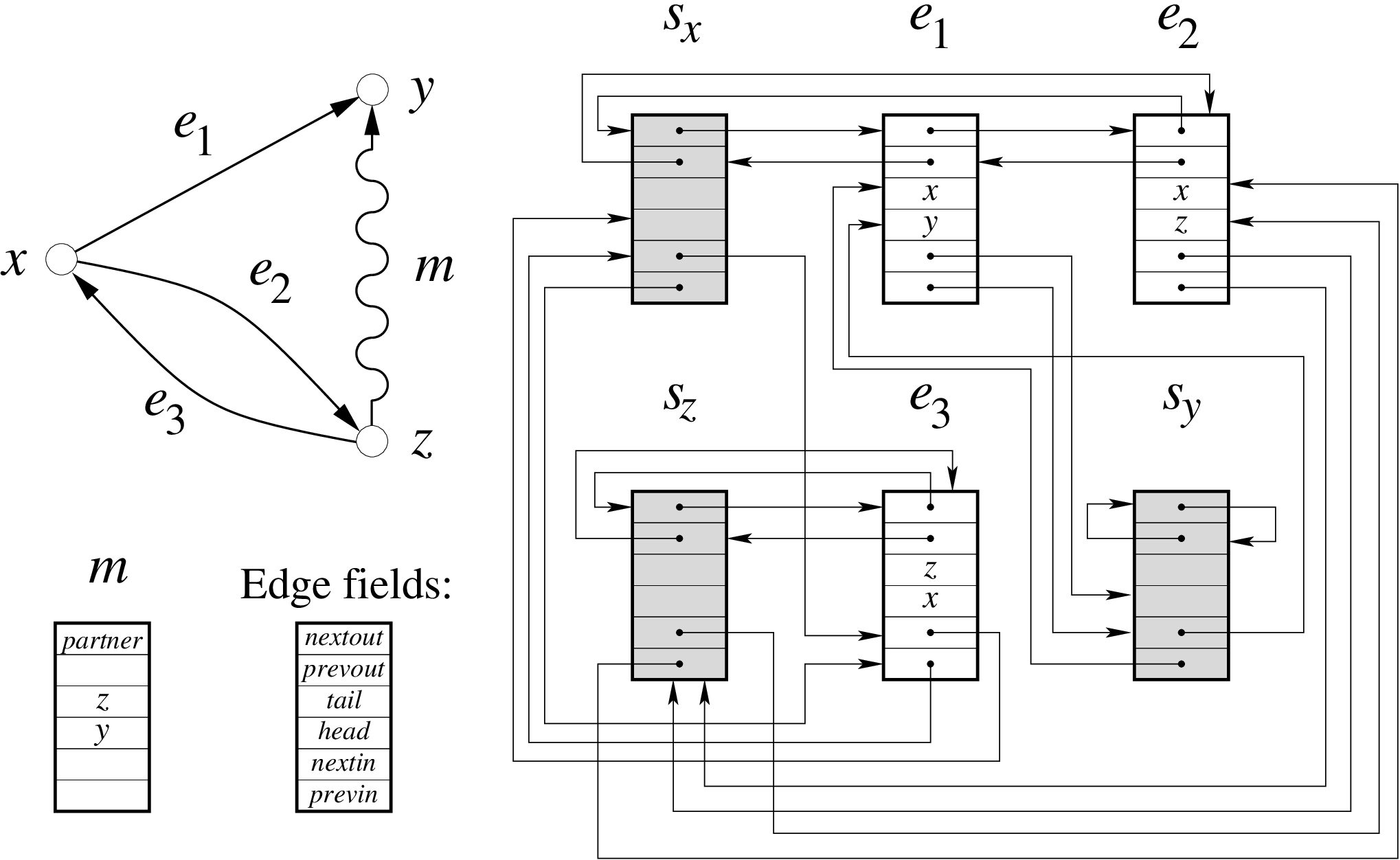
The list operations in lines 2, 8, 9 of shrink can be performed in constant time. For that purpose, it is useful to store the lists of outgoing and incoming unmatched edges of a node as doubly-linked circular lists that start with a “sentinel” (dummy edge), denoted by (see Cormen et al., 2001, Section 10.2). Figure 7 gives an example of small graph (which is neither Eulerian nor has a perfect matching). The three unmatched edges are and the matched edge is . The outlist of contains , the outlist of is empty, and the outlist of contains . The inlist of each node contains exactly one edge. The first and last element of the outlist of a node is pointed to by and , which are both itself when the list is empty, as for in the example. The inlist is similarly accessed via and . Each append operation in line 8 or 9 of shrink is then performed by changing four pointers. The remove operation in line 2 can, in fact, be done directly from , again by changing four pointers, here of the next and previous edge in the list (which may be a sentinel). Due to the sentinels, does not need the information of which node it is currently attached to, so line 2 should be written (a bit more obscurely) as “remove from its outlist” (that is, the outlist it is currently contained in), without reference to .
find_oppositely_signed_matching:
1 for all nodes
2
3
4
∗ 5
∗ 6
A : any matched edge of current graph
7
8
B :
9
10 if is not empty then
11 first edge in
12
13
14
15
16
17
18 else
19
20
21
22
23 if then
24 return
25
26
27 if then
28
29
30 else
31
Figure 8 shows the whole algorithm that finds a perfect matching of opposite sign via a sign-switching cycle. Initialization takes place in lines 1–6, which will be explained when the respective fields and variables are used.
The main computation starts at step A. The first node is the head of a matched edge. This assures that, due to the Euler property, this node has at least one outgoing unmatched edge that may be the first edge of an edge pair that is contracted with the shrink method. Starting from step B, a path of unmatched edges is grown with its nodes stored in where vc counts the number of visited nodes, and edges stored in , where is the edge from to for . A node is recognized as visited on that path when is positive, which is the index so that . This field is initialized in line 4 as initially zero (unvisited).
Line 10 tests if has a non-empty list of outgoing unmatched edges, which is true when . The next node, following the first edge of that list, is . Line 15 checks with the method checkvisited, shown in Figure 9, if has been visited before. If that is the case, then all edges in the corresponding cycle are completely removed from the graph and the nodes are marked as unvisited (lines 3 and 4 of checkvisited in Figure 9), and vc is reset to the beginning of that cycle. In any case, is the next node of the path, and the loop repeats at step B via line 17.
:
1 if then
2 for
3 remove from its outlist and inlist
4
5
Lines 18–31 deal with the case that has no outgoing unmatched edge, which can only hold if . Then the matched edge incident to is necessarily outgoing due to the Euler property and because has an incoming edge from to , which is found in line 22. This edge is normally removed in the shrink operation and then no longer part of the path, which is why vc is decremented in line 21 (node will no longer be part of the graph and can keep its visited field). However, a sign-switching cycle is found if (see Figure 10), which is tested in line 23 and dealt with in the expandcycle method called in line 24, which terminates the algorithm and will be explained below.

If , then is called in line 25. Afterwards, node is still the old representative of the head node of , as it was used in finding the path of unmatched edges. Node may be part of that path, as tested (and the possible cycle removed) in line 26. If has been visited, then because , so at least one edge is removed. If (which holds in particular if has not been visited), then the path is now grown from in line 28, where the find operation is needed to update in step B because the old representative may have been changed to after the unite operation in line 7 of shrink in Figure 5.
The case needs special treatment, which results in and happens when is same as the initial matched edge in step A. In that case, is removed via shrink, and may now be the tail rather than head of a matched edge, and then may no longer have an unmatched outgoing edge, which is necessary for lines 21–22 to work. For that reason, the loop goes back to A rather than B, as in line 31; note that has been set to zero in line 4 of checkvisited with . In step A, a new matched edge that has not yet been removed in a call to shrink can be found in constant time by storing all matched edges in a doubly-linked list (for example, using the fields nextin and previn that so far are unused for matched edges, see Figure 7); a matched edge should be deleted from that list after line 6 of shrink in Figure 5, for example.
:
1
2
3
4 for all
5 make a matched edge and an unmatched edge
6 return graph with this new matching
:
7 if then
8
9
10
11
12
We now discuss how to re-insert the contracted edges into the graph once a sign-switching cycle has been found, which is done in the expandcycle method in Figure 11. The method itself is straightforward. Recall that edges of the current graph are stored with the representatives of equivalence classes, where an unmatched edge is accessed in line 11 and a matched edge in line 19 of the main method find_oppositely_signed_matching in Figure 8. The sign-switching cycle will be reconstructed using the original endpoints of the edges. For each node , the original matched edge incident to is stored in (see line 3 of the main method), because may be modified (in line 10 of the shrink method).
In order to explain the expandcycle method, we record the time at which the shrink operation has been applied to a node . This is done in lines 3–5 in Figure 5 using using the field and the global variable sleepcounter, which are initialized in lines 5–6 of Figure 8. These lines have a “star” to indicate that they do not affect the algorithm, and can therefore be omitted. We use them to reason about the correctness of the expandcycle method.
The contraction affects three equivalence classes , , with representatives as shown in Figure 6. All nodes in become inaccessible afterwards, but the equivalence class still exists (and is in fact still represented in the union tree by those nodes so that , although the union-find data structure will no longer be used for these nodes). We say that all nodes in become asleep at the time recorded in the positive integer . Any node so that is called awake.
Lemma 15
During the main method find_oppositely_signed_matching, the following condition holds after any statement from step A onwards. Let be an equivalence class of nodes with representative and let . Then there is exactly one node in and another node not in so that:
(i) If is awake, then is awake and .
(ii) If is asleep, then is awake or asleep with later sleeptime than , and , .
In either case:
(iii) For every node in , let . Then , the node is asleep (with earlier sleeptime than if is asleep), there is an edge so that , the nodes and are equivalent and with we have .

Proof. We prove this by induction over the number of calls to the shrink method, which are the only times when the equivalence classes change. Initially, all equivalence classes are singletons and all nodes are awake. Then , only (i) applies, where is the matched edge incident to which is either the tail or head of and is the other endpoint of , and (iii) holds trivially.
Figure 12 shows the general case of the lemma. Consider the three equivalence classes , , with representatives as shown in Figure 6 in the notation used for the shrink method. Before is called, the lemma applies by inductive assumption to each of the three classes , , in place of . The unique matched edge that goes outside the equivalence class to an awake node is for and , and for it is some other matched edge (not shown in Figure 6) which will be that edge after and have been united. There is no edge other than or from a node in to an awake node outside because only in this case (when has in- and outdegree one in the reduced graph) the shrink method is called. Every node in , , or is the endpoint of a matched edge in the original graph, and other than the endpoints of and they are all equal to the head of such a matched edge, with its tail node asleep, by inductive assumption (iii).
After the shrink operation, and become a single equivalence class, and all nodes in becomes asleep. The only node in the new class for which (iii) does not hold by inductive assumption is , but then takes exactly the described role as . In particular, , because and and . In addition, changes its status from awake to asleep, and all nodes in are heads of matched edges that connect to equivalence classes that went asleep before as claimed in (iii) by the inductive hypothesis. This completes the induction.
The previous lemma implies that any two endpoints of a matched edge belong to different equivalence classes. A key observation in (iii) is that for any in an equivalence class that is not the endpoint of the “awake” matched edge there is another node different from in that class (which may be ) given by .
Lemma 16
Consider nodes and a set with the following properties: and are equivalent, and is the endpoint of an unmatched edge and is the endpoint of an oppositely oriented matched edge taken from the pairs of unmatched-matched edge pairs in , as in (i) or (ii) in Figure 13. Then after , the new edges in form a path of alternating matched-unmatched edges from to with the same number of matched and unmatched forward-pointing edges.

Proof. If , then the claim holds trivially with a path of zero length because no edge pairs are added to . Otherwise, we apply Lemma 15 to the equivalence class that contains and , as shown in the right picture in Figure 13, where takes the role of in Lemma 15(iii). Hence, node is the head of some matched edge with partner , and . Then in the method reconnect (line 10 in Figure 11), is added to . We then apply the claim recursively to instead of , and then to instead of , where the assumptions apply, exactly as in lines 11 and 12 of reconnect. So there are alternating paths as described from to and from to . The resulting path from to composed of these paths and the edges and has the same number of forward-pointing matched and unmatched edges, because and point in the same direction (in this case, backwards) along the path.
In the expandcycle method, lines 2 and 3 in Figure 11 call for the endpoints of the unmatched-edge pair shown in Figure 10 that results when expandcycle is called from the main method (line 24 of Figure 8), first for in and then for in in Figure 10. In both cases, Lemma 16 applies, and the paths together with the first edge pair form a sign-switching cycle.
Finally, exchanging the matched and unmatched edges as in line 5 of expandcycle can be done as described, irrespective of the order of the edges in the cycle, just using the pairs in (which are oriented in the same direction along the cycle), which suffices to obtain a matching of opposite sign.
This concludes the detailed description of the algorithm. It has near-linear running time in the number of edges, because each unmatched edge is visited at most once and either discarded or contracted in the course of the algorithm.

We illustrate the computation with an example shown in Figure 14. Suppose that edge lists contain edges in alphabetical order. The first node is 1. The first three iterations follow the unmatched edges , so that vc and the arrays visitednode and visitededge have the following contents:
Node 4 has an empty outlist, so that the computation continues at line 18 (all line numbers refer to the main method find_oppositely_signed_matching in Figure 8 unless specified otherwise). The matched edge is with endpoint , and is called in line 25. Afterwards,
and the reduced graph is shown in Figure 15. The nodes 3 and 5 have been united into the equivalence class which has representative because the unite operation in Figure 4 chooses the second representative if the original representatives have equal rank. The outgoing edges from node are and in that order, because the outlist of has been appended to that of .

In line 26, has no effect because . In line 28, , so that after going back to step B,
Line 11 then follows the unmatched edge with
after which again a contraction is needed, because is empty, this time with and call to . In the shrink method, returns because . The resulting graph, after line 25 is completed, is shown on the left in Figure 16, where
Now consider the call to in line 26 and note that is still the old node used before the contraction; recall that this is done because that representative is possibly stored in the visitednode array, which it indeed is at index . The deletion of the detected cycle of unmatched edges in lines 3 and 4 of checkvisited (see Figure 9) then produces the reduced graph shown on the right in Figure 16.


Normally, the next node would be in line 28. However, the case applies (recall the reason that the incoming matched edge of has been removed by the contraction), and so the computation continues via line 31 to step A. Suppose the first node is now 2. Then the computation follows edges and reaches node 8, with
Contraction with gives the graph shown on the left in Figure 17 where
and after the edge is removed, resulting in
This time, , so with we go back via line 29 to step B, after which
with the graph on the right in Figure 17.


Now has only the outgoing unmatched edge , giving in line 14 (where the last entry has not yet been assigned)
and removal of the edge gives the graph on the left of Figure 18. At the next iteration, after line 9,
where is empty, , and now in line 23. Now the final stage of the algorithm is called in line 24 with . The original endpoints of the two edges are (see Figure 14): , , , . Line 2 of Figure 11 makes the call which is nontrivial because with we have in line 7 of Figure 11. With and , we get (where is just our current name for the matched edge, with its original endpoints it is the edge ). All other calls to then have no effect because . The resulting sign-switching cycle is shown on the right in Figure 18.


In this example, every edge of the graph is visited during the algorithm, and the reduced graph at the end consists justs of the oppositely oriented unmatched and matched edge that define a trivial sign-switching cycle. The original graph in Figure 15 already has such an edge pair in the form of , which is not discovered by the described run of the algorithm. Here, not all matched edges and their partners that have been removed by the shrink operation are used (namely not and ). In other cases, the algorithm may also terminate with parts of the graph left unvisited, or unmatched edges in the visitededge array that are not removed.
References
Balthasar, A. V. (2009), Geometry and Equilibria in Bimatrix Games. PhD Thesis, London School of Economics.
Casetti, M. M., J. Merschen, and B. von Stengel (2010), Finding Gale strings. Electronic Notes in Discrete Mathematics 36, 1065–1072.
Cayley, A. (1849), Sur les déterminants gauches. Journal für die reine und angewandte Mathematik (Crelle’s Journal) 38, 93–96.
Chen, X., and X. Deng (2006), Settling the complexity of two-player Nash equilibrium. Proc. 47th FOCS, 261–272.
Cormen, T. H., C. E. Leiserson, R. L. Rivest, and C. Stein (2001), Introduction to Algorithms, Second Edition. MIT Press, Cambridge, MA.
Cottle, R. W., and G. B. Dantzig (1970), A generalization of the linear complementarity problem. J. Combinatorial Theory 8, 79–90.
Cottle, R. W., J.-S. Pang, and R. E. Stone (1992), The Linear Complementarity Problem. Academic Press, San Diego.
Daskalakis, C., P. W. Goldberg, and C. H. Papadimitriou (2009), The complexity of computing a Nash equilibrium. SIAM Journal on Computing 39, 195–259.
Eaves, B. C., and H. Scarf (1976), The solution of systems of piecewise linear equations. Mathematics of Operations Research 1, 1–27.
Edmonds, J. (1965), Paths, trees, and flowers. Canadian Journal of Mathematics 17, 449–467.
Edmonds, J. (2009), Euler complexes. In: Research Trends in Combinatorial Optimization, eds. W. Cook, L. Lovasz, and J. Vygen, Springer, Berlin, pp. 65–68.
Edmonds, J., S. Gaubert, and V. Gurvich (2010), Sperner oiks. Electronic Notes in Discrete Mathematics 36, 1273–1280.
Gale, D. (1963), Neighborly and cyclic polytopes. In: Convexity, Proc. Symposia in Pure Math., Vol. 7, ed. V. Klee, American Math. Soc., Providence, Rhode Island, 225–232.
Grigni, M. (2001), A Sperner lemma complete for PPA. Information Processing Letters 77, 255–259.
Hilton, P. J., and S. Wylie (1967), Homology Theory: An Introduction to Algebraic Topology. Cambridge University Press, Cambridge.
Jacobi, C. G. J. (1827), Ueber die Pfaffsche Methode, eine gewöhnliche lineäre Differentialgleichung zwischen Variabeln durch ein System von Gleichungen zu integriren. Journal für die reine und angewandte Mathematik (Crelle’s Journal) 2, 347–357.
Lax, P. D. (2007), Linear Algebra and Its Applications. Wiley, Hoboken, N.J.
Lemke, C. E. (1965), Bimatrix equilibrium points and mathematical programming. Management Science 11, 681–689.
Lemke, C. E., and Grotzinger, S. J. (1976), On generalizing Shapley’s index theory to labelled pseudomanifolds. Mathematical Programming 10, 245–262.
Lemke, C. E., and J. T. Howson, Jr. (1964), Equilibrium points of bimatrix games. Journal of the Society for Industrial and Applied Mathematics 12, 413–423.
Lovász, L., and M. D. Plummer (1986), Matching Theory. North-Holland, Amsterdam.
McLennan, A., and R. Tourky (2010), Simple complexity from imitation games. Games and Economic Behavior 68, 683–688.
Merschen, J. (2012), Nash Equilibria, Gale Strings, and Perfect Matchings. PhD Thesis, London School of Economics.
Morris, W. D., Jr. (1994), Lemke paths on simple polytopes. Mathematics of Operations Research 19, 780–789.
Papadimitriou, C. H. (1994), On the complexity of the parity argument and other inefficient proofs of existence. Journal of Computer and System Sciences 48, 498–532.
Parameswaran, S. (1954), Skew-symmetric determinants. American Mathematical Monthly 61, 116.
Robertson, N., P. D. Seymour, and R. Thomas (1999), Permanents, Pfaffian orientations, and even directed circuits. Annals of Mathematics 150, 929–975.
Savani, R., and B. von Stengel (2006), Hard-to-solve bimatrix games. Econometrica 74, 397–429.
Shapley, L. S. (1974), A note on the Lemke–Howson algorithm. Mathematical Programming Study 1: Pivoting and Extensions, 175–189.
Tarjan, R. E. (1975), Efficiency of a good but not linear set union algorithm. Journal of the ACM 22, 215–225.
Thomas, R. (2006), A survey of Pfaffian orientations of graphs. Proc. International Congress of Mathematicians, Madrid, Spain, Vol. III, European Mathematical Society, Zürich, 963-–984.
Todd, M. J. (1972), Abstract Complementary Pivot Theory. PhD Dissertation, Yale University.
Todd, M. J. (1974), A generalized complementary pivot algorithm. Mathematical Programming 6, 243–263.
Todd, M. J. (1976), Orientation in complementary pivot algorithms. Mathematics of Operations Research 1, 54–66.
Valiant, L. G. (1979), The complexity of computing the permanent. Theoretical Computer Science 8, 189–201.
Vazirani, V. V., and M. Yannakakis (1989), Pfaffian orientations, 0-1 permanents, and even cycles in directed graphs. Discrete Applied Mathematics 25, 179–190.
von Stengel, B. (1999), New maximal numbers of equilibria in bimatrix games. Discrete and Computational Geometry 21, 557–568.
von Stengel, B. (2002). Computing equilibria for two-person games. In: Handbook of Game Theory, Vol. 3, eds. R. J. Aumann and S. Hart, North-Holland, Amsterdam, 1723–1759.
Ziegler, G. M. (1995), Lectures on Polytopes. Springer, New York.